Contextual image classification

C ontextual Image Classification

Ian Poole

May 1991

(corrected version , M ay 1992)

Subm itted for the degree of PhD a t University College London

All rights reserved

INFORMATION TO ALL USERS

The qu ality of this repro d u ctio n is d e p e n d e n t upon the q u ality of the copy subm itted.

In the unlikely e v e n t that the a u th o r did not send a c o m p le te m anuscript and there are missing pages, these will be note d . Also, if m aterial had to be rem oved,

a n o te will in d ica te the deletion.

uest

ProQuest 10609353

Published by ProQuest LLC(2017). C op yrig ht of the Dissertation is held by the Author.

All rights reserved.

This work is protected against unauthorized copying under Title 17, United States C o d e M icroform Edition © ProQuest LLC.

ProQuest LLC.

789 East Eisenhower Parkway P.O. Box 1346

Abstract

This thesis studies some of the practical and theoretical issues arising in the contextual classification of image pixels.

The main practical contribution is a learning/classification system, named The system aims to:

• learn to exploit spatial characteristics such as texture, edge and line;

• learn to exploit contextual dependencies between classes;

• be efficient a t classification time;

• return ‘honest’ probabilistic assessments of classification confidence a t each pixel;

• exploit a parallel SIMD processor for classification.

The m ethod involves th e use of a genetic algorithm to search for ‘good’ partitions in a high-dimensioned p a tte rn space, th e partitions being built up hierarchically as a probability tree. This tree may then be used to produce a class probability image from similar te st data.

Probabilistic relaxation labelling (PRL) is a popular m ethod of iteratively refining proba­ bilistic assessments in the light of contextual constraints. A study of the theoretical limits of excellence for any PRL scheme is presented. The main result is th a t no scheme can produce assessments equivalent to those conditioned on all the d a ta in the image. It is also shown th a t for such a scheme to be optim al the updating function must be tailored for each itera­ tion and th a t after the first iteration the function will depend on the actual distributions of the raw data, not simply on the spatial correlation of the classes.

A new form of PRL - trained probabilistic relaxation (TPR) is presented th a t uses Lapwing to estim ate directly the updating function for each iteration in a particular do­ main of application.

Lapwing is dem onstrated on noisy synthetic texture discrimination, edge detection and on problems encountered in remote sensing and medical imaging, with encouraging results.

supervised

‘Lapwing’.

1 In tr o d u ctio n 13

1.1 Assumed k n o w le d g e ... 16

1.2 N otational co nv entions... 17

1.3 Outline of t h e s i s ... 17

1.4 A Survey of image classification in remote sensing ... 18

1.4.1 Per-pixel m e t h o d s ... 18

1.4.2 O bject c la ssifie rs... 20

1.4.3 Discrimination of t e x t u r e ... 21

1.4.4 Knowledge based c la s s ific a tio n ... 23

2 L apw ing - A n ew approach 25 2.1 Pixel versus object c la s s if ie r s ... 26

2.2 Specifying the p attern recognition problem ... 27

2.2.1 P a tte rn vector e x t r a c t i o n ... 27

2.2.2 F o rm u latio n ... 29

2.3 Honesty and r e f in e m e n t... 31

2.3.1 Overall h o n e s ty ... 32

2.3.2 Complete honesty (c a lib ra tio n )... 32

2.3.3 R e f in e m e n t... 33

2.3.4 R e m a rk s... 34

2.4 Conventional p attern recognition m e th o d s ... 34

2.4.1 N on-statistical m e t h o d s ... 35

2.4.2 Probability density function (p.d.f) estimation te c h n iq u e s ... 37

2.4.3 S u m m a r y ... 40

2.5 Lapwing’s probability tree a p p r o a c h ... 40

2.5.1 Constructing a probability t r e e ... 41

2.5.2 The splitting r u l e s ... 43

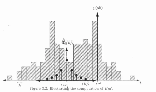
2.5.3 An additional criterion for resistance to simple bias - E m " { t )... 44

2.5.4 The to tal cost-function used by Lapwing ... 51

2.5.5 Searching — genetic alg o rith m s... 51

2.5.6 Tree validation and p r u n in g ... 54

2.5.7 C la ssific a tio n ... 56

2.6 S u m m a r y ... 56

2.6.1 Summary of the Lapwing technique ... 57

3 Im p le m en ta tio n d eta ils 59 3.1 Im plem entation on a serial machine ... 61

3.1.1 Tree generation — L E A R N E R ... 61

3.1.2 Tree validation and pruning — HONEST and P R U N E ... 64

3.1.3 Classification on the PC — C LA SSY ... 65

3.2 Classification on the Linear Array Processor (L A P )... 65

3.2.1 Introduction to the L A P ... 65

3.2.2 G eneration of P P L code for the L A P ... 6 6 3.2.3 LAP execution tim e s ... 67

3.3 Multiple class p r o b l e m s ... 67

3.4 S u m m a r y ... 67

4 E x p lo itin g co n te x t 69 4.1 Introduction to the Bayesian approach to c o n te x t... 70

4.1.1 The ‘message-centred’ sch em e... 70

4.1.2 The ‘object-centred’ sc h e m e ... 72

4.2 Introduction to probabilistic relaxation labeling ( P R L ) ... 73

4.3 A study of some theoretical limits on P R L ... 75

4.3.1 F o rm u latio n ... 75

4.3.2 Do per-pixel P P s preserve all relevant inform atio n?... 78

4.3.3 The incrementally optim al updating (IOU) scheme — g 1 . . ^ . . . . 81

4.3.4 Does the IOU scheme m atch a one-stage f u n c tio n ? ... 83

4.3.5 Towards closed-forms for gk ... 90 ~> 4.3.6 Graphical p r e s e n ta tio n s ... 91

4.3.7 The effect of iterating F1 ... 93

4.4 Trained probabilistic relaxation ( T P R ) ... 93

4.4.1 Claims to o p tim a lity ... 94

4.5 S u m m a r y ... 94

5.1.1 Artificial vs real te st im a g e s... 99

5.1 . 2 General notes on the conduct of t e s t s ...100

5.1.3 Performance s t a t i s t i c s ...100

5.2 Regular noisy texture d is c rim in a tio n ...103

5.2.1 Discussion of noisy texture t e s t s ... 104

5.3 Markov random field te x tu r e s ...106

5.3.1 G eneration of MRF t e x t u r e s ...107

5.3.2 Discussion of Markov texture t e s t s ... 109

5.4 Edge d e t e c t i o n ...115

5.4.1 Discussion of edge detection t e s t ... 115

5.5 Remotely sensed i m a g e r y ... 118

5.5.1 Discussion of ATM t e s t s ...119

5.6 Biological I m a g e s ...1 2 2 5.6.1 Discussion of biological image t e s t ... 122

5.7 Some e x p e r i m e n t s ... 125

5.7.1 The effect of training on an image which is more or less n o is y ... 125

5.7.2 Comparing T P R with a com putational PRL s c h e m e ...130

5.8 Entropy vs Classification e r r o r ...132

5.8.1 Relationship between P (error|A ) and H(Y]A) ...133

5.8.2 Discussion of entropy metric for preceding t e s t s ...134

5.9 S u m m a r y ...135

6 C on clu sion s 139 6 . 1 L a p w in g ... 139

6.1.1 P u ttin g Lapwing into c o n t e x t... 139

6.1.2 Further work ( 1 ) ... 140

6.2 PRL, IOU and T P R ... 141

6.2.1 Comparing PRL and T P R ... 141

6.2.2 Further work ( 2 ) ’. . . . 144

6.3 Concluding r e m a r k s ... 146

A G lossary 149 A .l A b b rev iatio n s... 149

A .2 N otation introduced in chapter 2 ...150

A .3 N otation introduced in chapter 4 ...151

A .3.1 A bbreviated notation used in p r o o f s ...152

B S ta tistic a l in d e p e n d e n c e diagram s (‘I-grap h s’) 153

C P r o o f o f th eo r em s 155

C .l Some theorem s in second level p r o b a b ilitie s ...155 C.2 Proofs for chapter 4 ... 157

^ D R E D U C E program and o u tp u t 163

1.1 Blewbury... 14

1.2 Them atic overlay... 15

2.1 ‘Inside box’ classification... 27

2.2 An example neighbourhood... 28

2.3 A variety of neighbourhood models ... 29

2.4 Example density functions on Q f... 32

2.5 H orizontal/vertical texture discrim ination... 35

2.6 The Parzen estim ator with Gaussian kernel... 38

2.7 k th Nearest-Neighbour density estim ation... 39

2.8 A probability tree and equivalent p artitio n... 42

2.9 Which are the b etter splits?... 44

2.10 Illustrating a problem with E m '(t) ... 50

2.11 Sketch of the function 4>o,r(b)... 50

2.12 A genetic a l g o r i t h m ... 53

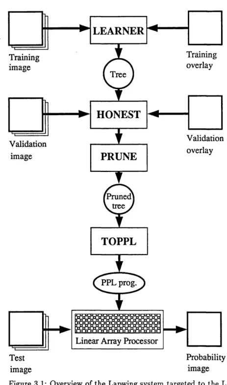
3.1 Overview of the Lapwing system targeted to the LAP... 60

3.2 Illustrating the com putation of E m 1... 63

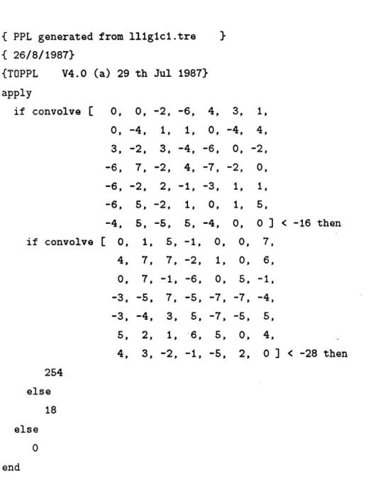
3.3 A small P P L p r o g r a m ... 6 6 3.4 A small probability tree as PPL c o d e ... 6 8 4.1 The I-graph for the tooth-comb model... 75

4.2 I-graph for the Hair-brush model... 77

4.3 Incrementally optim al updating ... 81

4.4 Simplified n otatio n ... 85

4.5 How to show th a t h is not a function... 87

4.6 Plots of min and max stage 2 P P s against 0... 92

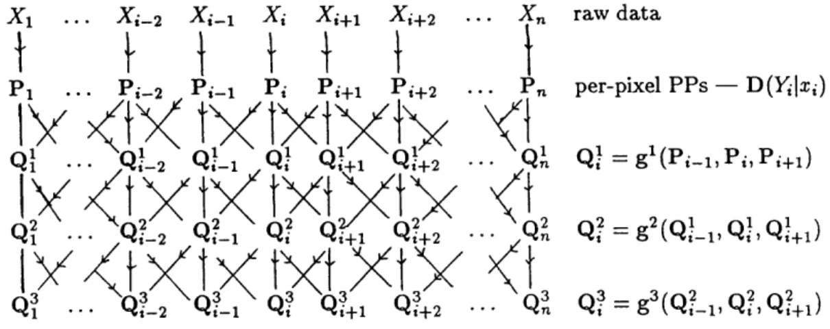
4.7 A data-flow diagram of T P R ... 95

4.8 Functional pseudo-code describing T P R ... 96

5.1 Inputs for te st 1 — vertical vs horizontal lines with 50% noise... 104

5.2 O u tp u ts for test 1 — vertical vs horizontal lines with 50% noise... 105

5.3 O u tp u ts for test 2— Vertical vs Horizontal lines with 100% noise...106

5.4 Exam ple MRF te x tu res...110

5.5 Inputs for te st 3 — Correlated vs un-correlated MRF textures... I l l 5.6 O u tp u ts for test 3— Correlated vs un-correlated MRF textures... 112

5.7 Results for test 4 — Directional small-scale MRF textures... 113

5.8 O u tp u ts for test 5 — Directional large-scale MRF textures... 114

5.9 Inputs for te st 6 — Edge detection...115

5.10 O u tp u ts for test 6 — Edge detection... 116

5.11 Inputs for test 7 — ATM... 119

5.12 Results for test 7 — ATM ...121

5.13 Inputs for test 8 — biological...123

5.14 O u tp u ts for test 8 — biological... 124

5.15 O u tp u ts for test 13 — ‘A ’... 127

5.16 O u tp u ts for test 13 — ‘B ’...128

5.17 C alibration curves after two iterations of T P R and H-PRL...131

5.18 S catter plots of Zf(Y|A) vs P ( e r r o r |A ) ... 137

B .l An example I-graph... 153

C .l To show th a t g2 depends on the d a ta distributions...159

C.2 D ata distributions yielding 3 non-zero points in d(at)...160

5.1 Results for test 1— Directional texture, 50% noise (test 9 in p aren .)... 103

5.2 Results for test 2— Directional texture, 100% noise (test 10 in p aren .) 107 5.3 Results for test 3 — Correlated vs un-correlated MRF tex tu res... 108

5.4 Results for test 4. — Directional small-scale MRF tex tu res... 108

5.5 Results for test 5. — Directional large-scale MRF tex tu res...109

5.6 Results for test 6 — Edge detection...117

5.7 Results for te st 7(test 1 1 in paren.)...118

5.8 Results for test 8(test 12 in paren.)...122

5.9 Results for te st 13 — ‘A ’ (test 14 results in paren .)... 129

5.10 Results for te st 13 — ‘B ’...129

5.11 Results for test 15 — H-PRL applied to ATM d a ta ...131

A great many people have contributed to this thesis, some of whom I shall try to mention. Gillian Peacegood has been a colleague and friend throughout the project, helping with my remote sensing problems, and offering many helpful comments. I am also grateful to the following people: Hilary Adams for introducing me to genetic algorithm s and making her GA code available; Phil Dawid for introducing me to belief networks and helping me with several statistical problems; John Crowcroft, Mark Handley, Valerie Isham, John Washbrook and Bill W itts for many and various stim ulating conversations, and Melanie Palm er for bringing to bear her editing skills on my contorted prose. T hanks also to the hardware and systems group of UCL CS for their excellent technical support.

Thanks to Graeme Wilkinson for initiating the project and to Piers Plumm er for his help with the LAP. Ed Brocklehurst provided supervision a t NPL. Financial support was provided by the SERC and NPL.

I am grateful to David Mason, Jeff Settle and their team a t NUTIS for making their ATM d a ta available to me; thanks also Richard Baldock a t the MRC for providing me with the electron-micrograph images; the image printing program was w ritten be James Pearson.

I would like to express my particular gratitude to Derek Long for having taken an active interest in my work, and for all his help and guidance with my many m athem atical difficulties.

Finally, a big thankyou to Paul O tto — the best supervisor any student could ask for. Paul has m aintained a close involvement in the project, providing me with ideas, advice, criticism and encouraged — all in m ost generous measure.

Dedicated to m y father,

David Poole

1924-1977,

in the hope th a t he would have been proud.

Introduction

Consider figure 1.1. This image was acquired from an airborne sensor and shows the town of Blewbury, in the Berkshire Downs, UK. 1

The image is composed of 512 x 512 picture elements — or pixels, each covering an area on th e ground of approximately 5 x 5 metres. The image shown is the 11th from a total of 1 1 registered images, or bands, each recording the intensity of reflectance in a particular range of the electromagnetic spectrum . The intensity a t each pixel is encoded in 8 bits (ie 256 possible intensity levels), thus the entire d a ta set comprises 512 x 512 x 11 x 8 = 22Mbits of d a ta.2

The potential uses for this d a ta axe many and varied — plotting of urban growth, mapping of wetland sites, prediction of national crop yields .. .etc. While it may be possible to fulfill these requirements by working from the raw image data, it will often be expedient to prepare first a thematic map from the data, in a m achine-readable form. The them atic m ap will label

each pixel with a category, or class, selected from a set of classes of interest to th e particular application. Figure 1.2 is such a m ap for the Blewbury image, distinguishing roads (black), cereals (light grey), urban area (dark grey) and ‘o th er’ (white). Questions such as “what proportion of cereal crop covers the area?” and “where are urban areas expanding (relative to an earlier im age)?” can be answered swiftly and mechanically. If the them atic map is sufficiently detailed (ie there is a fine division of classes) and accurate, then it could replace the original data; the them atic m ap has captured the significant meaning — the true

information contained in the data.

This thesis is concerned with th e autom atic preparation of such them atic maps, or over-1This image was acquired by the Natural Environment Research Council (NERC). The reference plane (fig. 1.2) was compiled by the NERC Unit for Them atic Information system s (NUTIS) (it has been simplified by the author).

2However the entropy of the data will be considerably less; this is what makes image compression (for storage or transmission) possible.

14 C H A P T E R 1. I N T R O D U C T I O N

Figure 1.1: Blewbury.

lays as they will be called. R em ote sensing applications will n ot be discussed in detail, although th e ty p e of tasks which have been m entioned probably c o n stitu te th e m ajor appli­ cation for these techniques; th e reader is invited to keep these concrete applications in mind as th e discussions becom e increasingly a b stra c t. O ther applications are m edical im aging (eg, labeling of abnorm al blood cells from a m icroscope image [Norgen81]) and in d u strial inspection (eg, identifying faults in rolled steel [Hill83], or perhaps gauging the proportion of fa t in a cu t of m eat).

W hile th e th em a tic overlay m ay be prepared by hand (indeed, this will often be th e only alte rn a tiv e ), there are obvious benefits of speed, objectivity and perhaps accuracy in m aking the tra n sitio n from im age d a ta to th em atic overlay a m echanical one. T his im m ediately raises some general questions:

Ifiiliil

Sxvxj:* .

Mm

SfeSpgi :?SSS:¥::

•iSisisSsi:

1II8IIIS

/

/

XVri.vx-iili

Figure 1.2: T h em atic overlay.

im age te x tu re can be exploited?

• Are contextual con strain ts to be considered — for exam ple, th a t forests occur as large areas, and roads are stra ig h t, thin, and more comm on near urban areas?

• Should the overlay be categoric or should it give some indication of th e certainty of th e classification?

• W h a t tim e con strain ts im pinge? Eg, m ust th e overlay be generated in real-tim e as the d a ta is captured?

• W h a t special hardw are architectures are available?

16 C H A P T E R 1. IN T R O D U C T IO N

processor (LA P). The LAP has a ‘single-instruction m ultiple-data’ (SIMD) architecture and was developed a t the National Physical Laboratories (NPL). An introduction to the LAP is provided in chapter 3.

1.1

A ssu m ed know ledge

It is clear th a t we are primarily concerned with a problem of pattern recognition. T h a t is, given some data A , associated with each pixel, assign to it a class Y.

This thesis cannot serve as an introduction to this large and rapidly developing discipline. There are many texts available to fulfill th a t role. Particularly useful for the beginner are [Duda72] and [Tou74]. For progressively more advanced texts see [Fukunaga72], [Patrick72] and [Devijver82],

It will be assumed th a t the reader is familiar with the basic term s an concepts of p attern recognition, such as a pattern vector,3 pattern space,4 decision fu n ctio n,5 supervised6 and

unsupervised7 recognition, and basic probability theory such as the a priori probability, 8 a

posteriori probability,9 conditional density10 and Bayes theoremn .

Knowledge of popular p attern recognition techniques such as the nearest neighbour (NN) , 12 minimum distance (MD) 13 and Gaussian maximum likelihood (GML) 14 classifiers will be useful.

3Pattern vector — the (usually multivariate) data upon which classification is to be based (A ).

4 Pattern space — the space of all possible values the pattern vector may take — visualise as a space with dimensionality equal to the number of components in the pattern space (fi).

5Decision function — assigns a given pattern vector to a class — essentially this is the classifier ( V( X) ) .

6 Supervised recognition — classified samples are available to train the classifier in advance.

7Unsupervised recognition — no classified training samples are available; we wish to assign similar pat­ terns to the sam e group or cluster.

8.4 priori probability — the probability of finding a particular class p rior to seeing any data (eg

P { Y = forest)).

9 A posteriori probability — our modified probabilistic assessment after (or given that) we have seen some data (eg, .P(Y =forest|x)).

10Conditional density — the probability density within a given class (eg p (X =x|Y =forest). 11 Bayes theorem - P ( y .f o r e s t |X « x ) = .

12NN classifier — assign a new pattern vector to the class of the sample to which it is closest in the pattern space.

13MD classifier — assign a new pattern to the class whose sample mean vector is closest in pattern space.

1.2

N ota tion al conventions

Random variables are w ritten in capitals (eg Y) and their realizations in lower case — eg, ?/;. Underscore is used for a joint list of variables — eg, y = ( y i. . . y n). Upper case ‘P ’ indicates the probability of a discrete event — eg P(Y=yt) reads “the probability th a t Y takes the value y f \ and D(Y) is the probability v e c t o r (or distribution) over all realizations of the discrete random variable Y. A variable which represents a probability vector is w ritten bold — eg, p t = D (Y jX =xt). A probability d e n s i t y on a continuous variable is indicated by p — as in p ( X = X {), w ith

d(X)

A glossary of notation may be found in appendix A.

1.3

O utline of thesis

In the following chapter the design goals for a supervised image classification system will be set out and a system, named Lapwing, developed to achieve them . The system delivers a probabilistic classification; a recurring theme will be the degree to which these probabilities are ‘honest’, and so a section is included th a t defines classifier honesty and related terms. Lapwing uses an optim ization technique (a genetic algorithm (GA)) to construct a probabil­ ity tree from training data. Im plem entation issues are addressed in chapter 3; in particular it is shown how classification may be performed on a linear array processor.

C hapter 4 contains the main theoretical results of the thesis. It considers ways of ex­ ploiting the contextual dependencies between classes to improve overall classifier confidence, and focuses on a particular and well studied technique — probabilistic relaxation labeling (PRL). Theorems are developed which establish a limit of excellence for this class of methods and highlight th e short-comings of existing implem entations. Some of the longer theorem proofs are removed and included in appendix C. Finally, a radically new scheme, tra in ed p r o b a b ilistic re la x a tio n (TPR ) is proposed which depends on Lapwing or a system like it for its im plem entation; this is th e unifying link between chapters 2 and 4.

Experim ental results from a variety of real and artificial problems are presented in chapter 5. T P R is compared with a particular version of PRL from the literature. The chapter also includes some discussion of the use of conditional entropy as a classifier perfor­ mance metric.

A short summary concludes each chapter, bu t more detailed discussion is presented in chapter 6.

A glossary of abbreviations and notation may be found in appendix A.

18 C H A P T E R 1. IN T R O D U C T IO N

proposed for remote sensing application.

1.4

A Survey of im age classification in rem ote sensing

In this section techniques are reviewed th a t are concerned with the ultim ate classification of image pixels. Work on contextual classification will be reviewed in chapter 4. This thesis is not concerned with image segmentation as such, though m ethods which involve segmentation as a pre-processing step to ultim ate classification will be looked at briefly.

See [Swain78b], [Curren85] or [Lillesand87] for introductory texts to remote sensing.

1 .4 .1 P e r - p ix e l m e t h o d s

Probably the most common classification methods used in remote sensing are those based on some form of statistical analysis of the d ata for each pixel in isolation. For these methods, all spatial aspects are entirely ignored; the image is treated as an unstructured ‘bag’ of pixels and so can usually be used only when some form of m ultivariate d a ta is available for each pixel (eg they would be inappropriate for panchromatic d ata). In rem ote sensing, this will usually be m ultispectral or possibly m ultitem poral data. Thus, the com ponents of the p attern vectors will be composed of the intensities in different spectral bands or at different times. Principal com ponent analysis will often be used first to select band components containing the greatest information.

A review of early work on remote sensing applications is provided in [Fu76], in which per- field classifiers, sequential p attern space partitioning (classification trees), cluster analysis and syntactic m ethods are discussed.

S u p e r v is e d m e th o d s

The m ost commonly used classifiers in remote sensing are the parellelopiped, MD and GM- L classifiers [Lillesand87]. Given the approxim ate normal distribution in spectral intensity space for carefully specified classes [Crane72] the GML decision surfaces would be expected to fit the class distributions more accurately than the cuboid regions implied by the par­ ellelopiped classifier. The MD classifier suffers from the assumptions of equal co-variances among the classes.

com putational load.

A hybrid of two classifiers can by used — use the parellelopiped classifier by default, resorting to the more costly GML classifier only where the cuboids of two classifiers overlap [Haberacker79]. A related technique involves the definition of two cuboid regions for each class, term ed the necessary and sufficient regions for th a t class [K0 0 8 6]. Only when the p a tte rn vector for a pixel falls in the cavity between the two regions is it necessary to evaluate the GML rule.

The efficiency of the GML classifier is tackled in a more direct m anner by [Feiveson83]. He describes a m ethod by which fixed probability thresholds can be pre-calculated for each class-conditional density function; if this probability is exceeded, then it is unnecessary to calculate the density functions of the remaining classes.

It is unlikely th a t every pixel in an image will be unique; it is, therefore, possible to avoid repeated com putation of a decision rule by function-memorization — storing the results in a lookup table as classification proceeds [Mather85]. The table can be implemented with a hashing algorithm to avoid unreasonable storage demands.

There have been several comparative studies to assess the efficacy of the various pattern recognition techniques to image classification in respect of both classification accuracy and com putational efficiency.

The GML classifier (with priors) is compared with linear discrim inant analysis for land use mapping in [Tom84], which concludes th a t the la tte r achieves greater classification ac­ curacy and reduced com putational load. This presumably implies th a t the assumption of Gaussian statistics was inappropriate in their application.

The performance of the GML and NN classifiers axe compared by Ince [Ince87], using Landsat TM data, with the conclusion th a t the NN classifier is significantly the more accurate due to the often inappropriateness of the Gaussian assumptions, and to th e problem of estim ating the param eters. However, he also comments, as do many other authors, on the practical difficulties of implementing the NN classifier in high-dimensional d a ta (his im plem entation involves a literal multi-dimensional array).

U n su p er v ised m e th o d s

20 C H A P T E R 1. IN T R O D U C T IO N

A clustering scheme for four-band m ultispectral d a ta is described in [Goldberg78]. A four-dimensional histogram is constructed using a hashing m ethod in order to avoid unreal­ istic storage demands. Histogram cells containing more than a certain threshold of observa­ tions are considered as peaks; peaks connected in p attern space are merged into one. The remaining cells are assigned to the nearest connected peak.

The ‘w atershed’ algorithm (see [Watson87]) is reminiscent of region-growing techniques used in image segm entation, b u t applied to the pattern space rath er than the image space. M ulti-band imagery m ust first be reduced to two dimensions by some suitable transform ation so th a t a bivariate histogram can be constructed on a hexadecimal grid. This histogram can then be treated as an ‘im age’. ‘B right’ points in this ‘im age’ are located and connected with any adjacent points th a t are ju s t one observation count lower. This is repeated for points th a t are two lower and so on. The result is a set of connected regions th a t can be arbitrarily labeled. The ‘im age’ can then be used as a lookup table to classify the (bivariate) observations.

1 .4 .2 O b j e c t c la s s ifie r s

The accuracy of classification can often be improved if homogeneous regions of the image are first identified by segmentation, and the combined statistics of all the pixels in the ‘o bject’ are used for its classification. Clearly, this approach depends crucially on the quality of the segmentation.

The prim ary example of this approach is the ECHO system — ‘Extraction and Classifica­ tion of Homogeneous O bjects’, described in [Kettig76] and [Landgrebe80]. The segmentation is achieved by first dividing the image into a regular grid of cells and then merging adjacent cells if they pass a statistical te st of similarity. The key to the classification stage lies in two assumptions: a) th a t the pixels of a region belong to the same class and b) th a t the obser­ vational d a ta is class-conditionally independent. These assumptions perm it the factorizing of the joint conditional density function for all the pixels into a product of their individual densities. A maximum-likelihood rule is then applied to the joint conditional densities. The appropriateness of th e class-conditional independence assumption is considered in [Poole8 8e]. 15 In [Kalayeh87], class-conditional correlation is tackled by modeling the interactions with a Markov mesh model. They develop modifications to MD and GML object classifiers, which take account of this model.

1 .4 .3 D is c r im in a t io n o f t e x t u r e

Many authors (eg [Palgen70], [Mason87], [Alm85]) have remarked th a t classification methods th a t ignore the spatial features of the image — as do the m ethods described so far — are severely limited in their discrim inatory power. Clearly they cannot discriminate texture.

Texture classification may become increasingly significant in remote sensing with the advent of 10-meter resolution, panchromatic d a ta provided by the SPO T satellite.

Enrich and Foith [Enrich78] list three issues with which researchers have been inter­ ested concerning texture: texture classification, texture modelling (synthesis) and texture segm entation. It is the la tte r of these th a t has been the dom inant subject of research in recent years. Here we must confine ourselves to only the former. However, b o th classifi­ cation and segmentation require the extraction of features th a t will perm it discrimination between two differently textured regions. Haralick [Haralick79] surveys many approaches to deriving tex ture features and categorises them into ‘optical transform s, digital transforms, textural edginess, structural element, grey tone co-occurrence, run lengths and autoregressive models’. The review has been expanded and updated in [Haralick8 6a].

Various statistical features for describing texture are discussed by Chen and Pavlidis [Chen79]. First-order statistics are concerned with only the frequency distribution of the grey levels in the image. These include the mean, variance, skewness and kurtosis.

Second-order statistics are concerned with the joint intensity distributions of pairs of pixels separated by a given displacement (&r, 8y). For each displacement these statistics can be captured by a

co-occurrence m atrix. These are similar to the ‘grey-tone, spatial-dependence m atrices’ first proposed by Haralick et al [Haralick73]. The (i j ) t h entry of this m atrix gives the probability of finding a pixel of intensity i, with a pixel of intensity j a t a displacement of (6x, 8y) from it (assuming a stationary image field). The m atrix is symmetric. Typically, the number of significant intensity levels is reduced (eg to eight) for obvious storage and sampling reasons. Chen and Pavlidis simplify the situation further by considering values for (8 x, 6y) of only (0,1), (1,1), (1,0) and (1,-1), and forming a sum of these four matrices. (Note th a t the summing discards any directional information, which may or may not be desirable.) As they are concerned with segmentation, they define a similarity measure between two matrices to establish whether two m atrices derive from the same texture. In later work [Chen83] they use the correlation between displaced pixels in place of co-occurrence matrices. They assume th a t the jo in t intensities of the pixels a t a given displacement follow a Gaussian distribution and thus can be described by a two entry mean vector and a 2 x 2 co-variance m atrix. For any given region, these can be estim ated directly.

auto-22 C H A P T E R 1. IN T R O D U C T IO N

matic image analysis, Rosenfeld [Rosenfeld62] uses analog techniques to analyze the spatial frequency of the intensities across scanned lines of aerial photographs. This technique has been further developed in [Idelsohn70] to produce a trainable classifier. The approach gen­ eralises to the digitally com puted two dimensional Fourier transform of a (sub) image and is described in many places — see [Bajesy73a], [Harris80] [Ballard82]. Fourier features based on phase are less useful for texture classification than those based on am plitude [Eklundh79]. It also appears th a t Fourier features in general are inferior to the first and second order statistics described above, for terrain classification [Weszka76].

A very different approach to obtaining texture feature is proposed by Laws [LawsSO] and further developed by Pietikainen et al [Pietikainen83]. This involves a set of zero summing 5 x 5 convolution masks which are derived systematically from simple one dimensional masks. Laws selected the eight most useful from the set. These are convolved in tu rn with a sub image (which is assumed to be texturally homogeneous) and the sum of the resulting absolute intensities is calculated for each. These eight values form a feature vector for treatm ent by an appropriate classifier.

The m ethod of ‘adaptive windows’ [Aleksander82], [Aleksander83] has been applied to texture discrimination by Kani and Wilson [Kani87]. Following is a brief description of the adaptive window (or ‘W IZARD’ nets as they are commonly known).

Sets of random access memories (RAMs) are addressed by randomly selected pixels from a region of a binary image. There is one set of RAMs (each identically connected) for each p attern class of interest. During training several patterns are presented to the system and th e RAM set of the associated p attern class is write-enabled. At classification time, with the RAMs in read-mode, ou tp u ts of each RAM are summed within each class set and the m ost voted-for class is chosen. It is the speed with which the discriminators can be trained and applied th a t constitutes the main advantage of the method. The ‘confidence’ of a particular decision is related to the relative number of votes of the ‘w inner’ and ‘runner- up ’. In [Aleksander6 8], [Aleksander83], [Kani87] and [Masih8 8], a feedback mechanism is described which dem onstrably improves the ‘confidence’ of the decision. However, it is by no. means obvious th a t the reported increase in confidence need have any relationship w ith actual improvement in classification accuracy, since the feedback incorporates no new information.

1 .4 .4 K n o w le d g e b a s e d c la s s if ic a t io n

The m ethods described so far have been, loosely, statistical. In addition, there have been attem p ts to apply artificial intelligence techniques (see eg [Charniak85]) to the task of image interpretation. As this can ultim ately produce pixel classification, some of this work will be mentioned here. A common feature of these systems is th a t they work at the object level, these objects having been first identified by some initial segm entation process. They are largely model a n d /o r rule based. A reviews can be found in [Binford82j.

Nagao et al [Nagao79a] describe a system for the interpretation of aerial photographs. An initial segm entation first roughly categorises the scene into a) large homogeneous regions b) elongated regions c) large vegetation regions d) high contrast regions. Each of these groups is then analyzed in greater detail by knowledge base modules tailored for each type. A further stage then improves on the initial region classification in the light of the classification of neighbouring regions. While good results were dem onstrated, the techniques used are largely ad-hoc.

The system described by Nazif and Levine [Nazif84] is independent of domain, and is intended for image segmentation. Rules operate on image primitives such as line segments and regions to establish a consistent interpretation. A further set of ‘m eta-rules’ control, and focus the attention of, the system.

Peacegood [Peacegood89] applies knowledge-base techniques to the task of detecting linear features (road, river, railway, field boundary etc) in aerial imagery. During a pre­ processing stage, edge and line segments axe detected and placed into a relational data-base. A collection of domain specific rules then act on this data-base, using relationships such as ‘is parallel to ...’, ‘is straig h t’ etc, to generate a probabilistic classification of each line/edge segment. A final stage involves the construction of a Bayesian belief network [Pearl8 8] to update the initial classification in view of contextual dependencies between spatially related segments.

Lapwing - A new approach

In this chapter a novel means for performing supervised image classification is developed, intended to satisfy the following design goals.

1. The system should be trainable by example to a wide range of applications.

2. It should take account of local spatial features such as texture, edge and line, as well as inform ation from m ulti-band imagery (multi-sensor, m ulti-spectral etc).

3. Potentially subtle contextual dependencies between classes should be learnt and ex­ ploited where they exist.

4. The classifier should yield a probabilistic assessment of its confidence; th a t is, we require the a posteriori probability (PP) vector for each pixel.

5. The m ethods used should be efficient at classification time and suitable for implemen­ tatio n on parallel SIMD architectures to improve speed further.

The case for goal 4 may not be obvious. It shall in fact become clear in chapter 4, th a t the existence of a classifier th a t generates (class conditional) a posteriori probabilities (PPs), on the basis of spatial relationships, is a vital requirement for the im plem entation of the context exploiting scheme which will be presented in th a t chapter; ie, it is a pre-requisite to goal 3. In any case, the P P s, when displayed as grey tones or pseudo-colour, can be useful for the hum an interpretation of the classifier’s results. Furtherm ore, the a posteriori probability is the measure which retains all information relevant to the specified classes, (see eg [Dawid85]; see also lemma 1 1 in appendix C).

The layout of this chapter is as follows. Section 2 . 1 discusses the dichotomy of pixel and object-based approaches. Section 2 . 2 specifies the p attern vector and formulates the problem in term s of classical p attern recognition. Section 2.3 pauses to consider the issue of classifier

honesty which will be a recurring them e throughout this thesis. Conventional solutions to

26 C H A P T E R 2. L A P W IN G - A N E W A P P R O A C H

the problem formulated in §2.2 are considered in §2.4. The solution finally adopted for Lapwing is then described in detail in §2.5, and the m ethod is summarized in §2.6.

2.1

P ixel versus object classifiers

It was observed in the introductory chapter th a t image analysis — leading to ultim ate pixel classification — can be approached in two very different ways:

• by classifying on a per-pixel basis, possibly taking into account neighbouring pixels (see §1.4.1);

• by segmenting out ‘objects’ (regions) and then assigning all the pixels in each object to the same class based on inform ation derived from the whole object (see §1.4.2 and §1.4.4).

The prim ary advantage of the la tte r approach is th a t higher level features can be used when making the classification — for example, shape features such as area/perim eter factors, [Mason87] [Nagao80] or the presence of right-angles [Mckeown85]. A lternative representa­ tions of shape may be used, such as the Fourier description [Brill6 8], or the Hough transform [Hough62] [Duda72] [Leavers8 6bj. If the objects are line segments, then line length and sinu­ osity (the ratio of length to end separation) may be helpful (see eg [Peacegood89]). Features may also be derived from various aggregates of the pixel intensities within the object, such as simple first order statistics (eg mean and variance) [Mason87], second order-statistics from co-occurrence m atrices [Chen79] or features from the fourier spectrum [Harris80j.

It has become custom ary to deride per-pixel classifiers as being over simplistic — never­ theless, this is the strategy adopted in this thesis, for the following reasons:

• O bject classifiers are crucially dependent on the quality of the initial segmentation. From the plethora of work th a t continues to be published on the topic (see [Haralick85] and [Rosenfeld8 8] for reviews), it may be concluded th a t the segmentation problem remains far from solved; no definitive segmentation m ethod has yet

se g m e n te d . (See [Reynolds83] for an approach to this involving th e in teraction of a hum an o p e ra to r).

• Per-pixel schem es are more appropriately im plem ented on SIMD arc h ite c tu re s as there is an obvious m apping — a pixel (or column of pixels) per processor. (However, see [Otto86] for th e im plem entation of various object based algorithm s on such m achines).

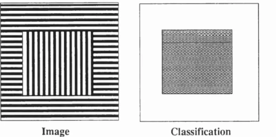
R aster scanned im ages in their raw form are arrays of picture elem ents, th u s any scheme m u st ultim ately be expressible as a function of the pixel intensities. O b ject classifiers perm it th e classification of a pixel to be influenced by an intensity which is rem ote from it. Consider for exam ple th e som ew hat perverse task of classifying pixels as being inside a rectangle, as shown in fig. 2.1. Clearly this problem is m ost sensibly tackled by an object based scheme,

Intensity here can affect classification here

C lassification Im age

Figure 2.1: ‘Inside b o x ’ classification.

however, provided a per-pixel classifier is endowed w ith a window twice th e size of the largest box, th en , when this window is centered on any point inside a box, th e whole box will be ‘visible’, and th e p o ten tia l for correct classification exists, a t least in principle.

T he rem ainder of this thesis is concerned w ith per-pixel classification techniques.

2.2

Specifying th e p a t t e r n recognition p ro b lem

2 .2 .1 P a t t e r n v e c t o r e x t r a c t i o n

28 C H A P T E R 2. L A P W IN G - A N E W A P P R O A C H

the neighbourhood model. Possible choices include the whole image (!), a random (fixed) s- election around the pixel (as with W izard [Aleksander83]), or a pre-determined window. Lapwing uses the latter, though a small degree of sophistication is introduced in order to extract information at multiple resolutions, and as a minor sop to efficiency.

Lapwing’s neighbourhood size can be varied, b ut is essentially of the form shown in fig. 2.2. In this case, 18 values are extracted, 9 directly from the central region, plus 9

*7 4 *75 *72

* / 5

* 5 *4 *3

* / /

* 7*8Xg

* 7 6 * 7 7 *78

18

= X

Figure 2.2: An example neighbourhood.

averages (arithm etic mean) from the outer 3 x 3 squares (the central 3 x 3 average is designated x 10, bu t is not shown in the diagram ). This arrangem ent allows the perception of fine detail a t the centre, as well as coarse structure a t a greater distance, whilst keeping the num ber of features, d, within reasonable bounds (d = 18 rather than 81).

The neighbourhood ju s t described is based on a 3 x 3 grid, extracted a t two resolutions. We can generalize within this basic structure, denoting by Mw the width of the basic neigh­ bourhood, and by A/) the num ber of resolution levels used. Thus, the neighbourhood model of figure 2.2 can be specified by Afw = 3, A/i = 2. Figure 2.3 shows some other possibilities. W hen multi-band imagery is used, the described neighbourhood is extracted from each band, multiplying the vector size accordingly. For notational completeness then, we may write the number of bands to be used as A/^. Thus, conventional per-pixel schemes used in remote sensing on, say, five band imagery, use a neighbourhood model Afw = 1, Mi = 1, Mb = 5. The ability to accept more than one input image also perm its pre-processed versions of the image — a variance transform for example — to be presented to the system when it is suspected th a t this may be useful. Clearly these neighbourhoods generate a vector of size

d = Afb • Afi - Afw 2 and cover Afb • (N w * A/})2 raw pixel values. It m ust be stressed th a t

Afw = 3 , M = l ATw = 5, t f i = l

^ = 3 ,^ = 3

2 .2 .2 F o r m u la tio n

P a tte r n v ecto r —

An image is a collection of N j pixels T = {i\i = l . . N j } . W ith each pixel i is associated its pattern vector x; extracted from the image in the m anner described in the previous section (so for the neighbourhood system shown in fig. 2.2, each x t has 18 components). The associated (vector valued) random variable is w ritten X . T he order of the components in the p attern vector can be inferred from the diagrams; it is clearly arbitrary. The space of

all possible vectors is a continuous d dimensioned hyperspace, term ed the pattern space, and denoted Q; x^ E O. Each component of x t takes values from the range [0, /].1

P a tte r n class — y E $

Also associated with each pixel i is its class y{. The set of all possible classes is $ = { l . . . m } — meaning eg {urban, forest, w ater ...}. The associated random variable is w ritten Y. As a notational convenience, we will often w rite

y,-

T raining sa m p le — C

The training (or ‘le a r n in g ’) sample is presented to the system in the form of an example image (or image stack) in conjunction with a registered training overlay which indicates the tru e class for each pixel. We have already m et an example of an image/overlay pair in figures

*In practice, Cl will be a discrete space, with the vector com ponents typically taking values from the

set {0..255} (ie 8-bit pixel data); it is convenient however to treat the space as being continuous for the

30 C H A P T E R 2. L A P W IN G - A N E W A P P R O A C H

1.1 / l . 2. From these it is possible to obtain for each pixel i, realizations of its class ?/, and p attern vector x,- (except th a t pixels a t a distance of Afw • A/} or less from the edge may not be used, thus C is taken to exclude these marginal pixels). Formally then, the training sample 2 is a set of N c pairs;

£

= {(x,•,&■)!* =

Note th a t unless Afw = A/} = 1 the sample-points will not be independent since their p attern vectors will overlap.

T h e p r o b le m

We can now pose our task succinctly:

Find the best refined and honest (see below) estimate of the a posteriori prob­ ability vector D (Y |X = x), fo r any x 6 based on the training sample C.

Providing th e prior probabilities D(Y) are available, it would be sufficient to find the condi­ tional density functions d(X|Y=a;) Va G $ since by Bayes’ theorem:

F ( y - o lx ) - P(x\Y=<*)-P(Y=ai)

1

'

’ ~

E^*P(x|y=/3).P(y=/3)'

(

’

The decision function, P (x ) € $ then follows immediately either by —

P (x ) = a if P(Y=<*|x) = m axP(Y =/3|x) (2.2)

or by —

P (x ) = a if p(x|Y=q;).P(Y=q;) = maxp(x|Y=/3).P(Y=/3) (2.3)

The first form is commonly term ed the maximum a posteriori probability (MAP) rule, and the second the Bayes rule, though they are equivalent by 2.1 — the normalizing denom inator does not depend on a and so can be dropped.3

The problem has been stated in statistical p attern recognition terms. A similar formula­ tion, for tem plate matching, is alluded to by [Duda73, §7.5.2], however they comment th a t ‘the application of formal statistical m ethods to problems of detecting objects in pictures

2 By sample we intend the usual statistical meaning — ie a collection of ‘units’ drawn from a population (see eg [Cochran63]). Our population is the set of all ‘units’ (ie pattern vector / class pairs) which the system may be called upon to deal with. Our sampling technique consists in manually selecting a single image which we judge to contain a representative set of these ‘units’. We cannot therefore claim to have a strictly random sample of our population, but will treat it as such. In this thesis we will use the term point

or sample-point to refer to a single ‘unit’.

has proved difficult in practice’. They consider the problem to be tractable only if the dis­ tribution of intensities can be considered as statistically independent, thus perm itting the factorizing of the joint distributions.

Before going on to consider conventional solutions to this problem, a digression —

2.3

H on esty and refinem ent

Questions concerning the honesty of a classifier a will occur frequently; this section establishes the statistical grounding of th e concept and relates it to similar term s use by other authors. A full discussion of these issues may be found in [Dawid85] and [Dawid86] — the la tte r being a particularly readable account. Dawid’s discussion relates to probabilistic ‘forecasting’ — taking the particular example of weather forecasting. In the Unites States it is common practice to issue a ‘probability of precipitation’ (‘P o P ’), and the techniques to be described in this section are used routinely to ensure the honesty of these predictions.

The honesty of a classifier becomes an issue only when it claims to deliver a probabilistic

assessment of its decision — ie when it adm its to, and attem p ts to quantify, its own uncer­ tainty. The question then arises: “how honest is the classifier being in its admissions?” .

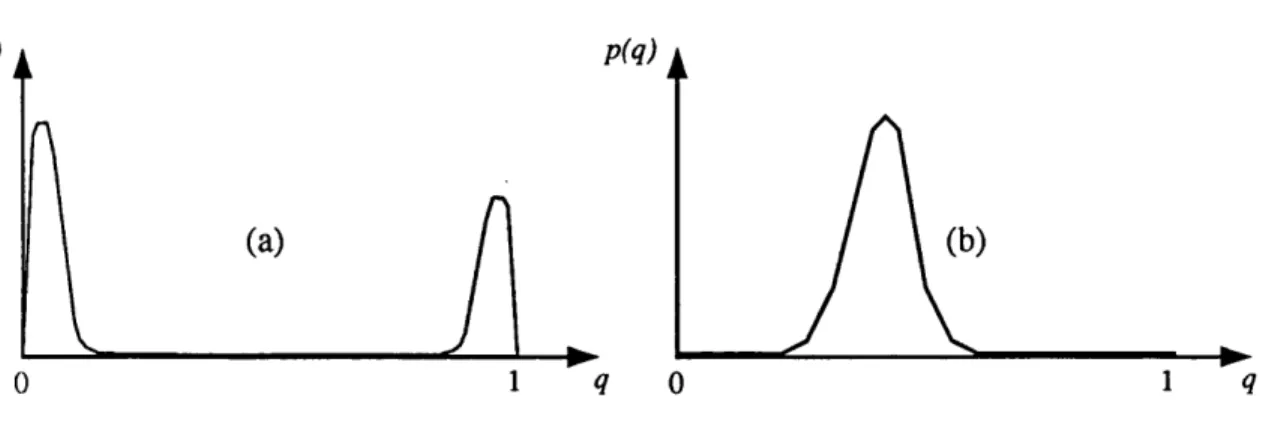
Consider the three-class classifier — $ = {fo r e s t, urban, other} — th a t returns a quan­ tity Q a t each pixel which it claims represents the a posteriori probability vector on Y, given some d a ta A (realization w ritten 6). We consider Q to be a random variable (functionally dependent on A ), realizations of which will be w ritten q. So the classifier claims:

Q = D (Y |A ).

Let the com ponent of Q relating to forest be Qf. Suppose th a t on examining a random sample of Q f realizations from the classifier we observe numbers such as .04, .07, .92, .02, .91, .97 etc. The classifier invariably returns probabilities which are very close to zero or one, indicating a high degree of confidence th a t the MAP decision based on these values will be correct. The distribution d(Qf) for this classifier m ight look like th a t of figure fig. 2.4 (a). A nother classifier (using different d a ta perhaps) might generate Qf

values such as .33,

32 C H A P T E R 2. L A P W IN G - A N E W A P P R O A C H

p(q)

1 0 1

0

Figure 2.4: Example density functions on Q j.

in fact tu rned out to be correct 95% of the time then we would conclude th a t it is also being dishonest in delivering overly cautious, or pessimistic predictions.

The following two sub-sections define two criteria coined overall honesty and complete honesty; the la tte r is th e more dem anding and encompasses the former.

2 .3 .1 O v e r a l l h o n e s t y

A truly honest classifier is capable of predicting its own error-rate — the percentage of its incorrect MAP decisions — over a given sample. It is easy to show (see §5.1.3) th a t for a classifier which delivers genuine a posteriori probability vectors q t- a t each pixel i —

53

predicted error-rate = ( 1 --- )

where <7,-£>(q.) is the com ponent of q t selected by the MAP decision rule — ie the highest valued com ponent. It should be emphasised th a t predicted error-rate (as w ith actual error- rate) is a quantity attached to a particular te st set — it will not in general be the same as the error rate expected over the entire population.

The actual accuracy is simply the percentage of pixels incorrectly classified (by X>(Q)) as com pared with ground tru th . Overall honesty is the requirement th at:

predicted error-rate « actual error-rate.

How different these figures m ust be before we conclude th a t the classifier is significantly dishonest is not addressed — the two quantities will simply be compared subjectively.

2 .3 .2 C o m p l e t e h o n e s t y ( c a l i b r a t i o n )

0.15 and 0.25 say), 20% are in fact forest. Thus, complete honesty requires:

P{Y=y\Qy=q) sa g,V3 € [0,1], Vy € $ . (2.4)

Again we do not address questions concerning the required strength of the equalities. Dawid [Dawid86] lists the term s ‘unbiased in th e small’, ‘reliable’, ‘valid’ and ‘well cal­ ib rated ’ as having been used in the statistical literature to describe this strict requirement for honesty. The calibration of a classifier may be displayed as a ‘calibration curve’ (see [Dawid86], also suggested in [Poole88e]) which plots P ( Y = y\Qy = q) against q. Separate curves are plotted for each class in multiclass problems. Examples of a calibration curve for an honest and a dishonest classifier may be seen in figures 5.17 (a) and (b) respectively.

A classifier returning any genuine probabilistic quantity will be a priori well calibrated regardless of its conditioning. For example, the quantity Qr = P (rain | DAY-OF-WEEK) will be perfectly honest — b u t of little use! Dishonesty may arise either when probabilities are obtained subjectively, when estim ations are made from a sample of insufficient size (for the fitted model), or when they are computed under statistical assum ptions th a t are not entirely valid.

2 .3 .3 R e f i n e m e n t

Suppose a (multi-class) classifier claims to deliver the vector quantity

Q = D (Y |A )

and we wish to verify the tru th of this claim. Firstly, Q claims to be a probabilistic quantity and so we require it to be well calibrated and satisfy condition 2.4. B ut this is not sufficient to verify the classifier’s claim since as has already been remarked, this will be satisfied by any probability (on Y) — the prior probability D(Y) for example! If th e classifier claims th a t Q is already fully conditioned on A then we should also find th a t A gives us no more inform ation about Y than does Q, so th at:

D (y |Q = q , A=fi) « D (Y lQ =q),V q,W .

W hen a classifier is completely honest, b u t does not satisfy the above criterion we say th a t it is not fully refined on the d a ta A. This will arise, for example, when the width of the kernel used by the Parzen estim ator (discussed in §2.4.2) is too great, or, as shall be seen in §2.5.6, when a probability tree is pruned back too severely.

34 C H A P T E R 2. L A P W IN G - A N E W A P P R O A C H

It is possible for a classifier to be perfectly refined on the d a ta A and yet not be honest. In this case the classifier is capturing all the information contained in A and relevant to V, b u t is not delivering a posteriori probabilities. In such cases the classifier m ust be delivering some reversible function of the a posteriori probability and thus it will usually be a simple m a tter to re-calibrate the classifier after observing its outputs on test d ata for which the tru e classification is available. The re-calibration process is equivalent to training a second classifier on the o u tp u t of the refined b ut dishonest classifier.

2 .3 .4 R e m a r k s

Several advantages accrue to a classifier which returns an honest probabilistic assessment:

• As has been seen, it can predict its own error rate over a particular test set (not ju st in general).

• A decision might have ‘economic’ consequences, presenting a so-called ‘cost-loss’ prob­ lem. It is shown in [Dawid86], th a t only by delivering the completely honest a poste­ riori probability vector, can these decisions be taken in a statistically justifiable way.

• W hen the results of a classifier axe to be post-processed, to take account of contextual constraints, for example, probabilistic reasoning can only be applied if the classifier delivers genuine (completely honest) probabilistic quantities.

• For an im portant application one might consider using several classifiers — each based on different features perhaps, or employing different techniques. It is then quite possible th a t each classifier will be well refined in some regions of the p attern space but poorly refined in others, b u t th a t these regions are different for each classifier. Providing the classifiers deliver completely honest P P s it would be reasonable to select the MAP decision of the most confident classifier, in each case. Clearly this would be meaningless if one or all of the classifiers were being wildly under- or over-confident.

In the Results and evaluation chapter, bo th the actual and predicted error-rates will be given, perm itting the overall honesty of the P P s generated by Lapwing to be assessed.

2.4

C onventional p attern recognition m ethods

Im age C lassification

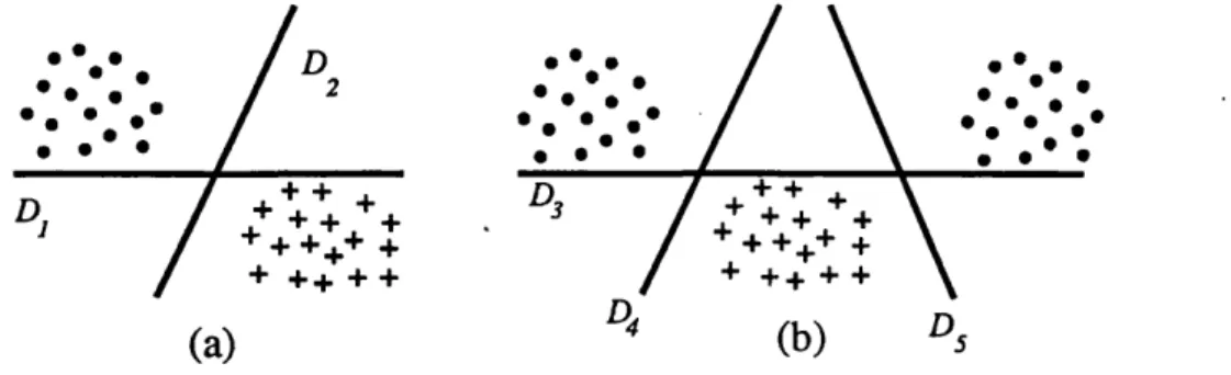
Figure 2.5: H o rizontal/vertical te x tu re discrim ination.

are exactly one pixel wide and one a p a rt, then b o th classes will have two m odes, eg, for the vertical class, (with Afw = 3, Mi = 1) and assum ing binary data:

0 1 0 1 0 1

0 1 0 or 1 0 1

0 1 0 1 0 1.

In fact th e problem can be reduced to th e ‘exclusive o r ’ type which is easily shown to be linearly inseparable 4 (see [Minsk/88, §2.1]).5

We will now consider the appropriateness of a num ber of ‘s ta n d a rd ’ p a tte rn recogni­ tion techniques to the form ulated problem , paying p articu la r a tte n tio n to their efficiency at classification tim e (goal 5).

Some techniques are ‘n o n -sta tistic al’ in th a t they deliver th e decision function V(. ) di­ rectly, ie w ith o u t generating th e a posteriori (or conditional density) d istrib u tio n s. Although these m eth o d s im m ediately fail to satisfy us (goal 4), it will be in stru ctiv e to consider them briefly.

2 .4 .1 N o n - s t a t i s t i c a l m e t h o d s

In [Minski88, c h .12] th e following n o n -statistical p a tte rn recognition m ethods are discussed:

• Linear discrim inants via:

— th e ‘B est p lan e’

- th e ‘P e rce p tro n ’ procedure

— since it is not possible to find two weights a, 6 such th a t a .l -f 6.0 > 1, a.O + 6.1 > 1 and a .l + 6.1 < 1. 5N ote th a t the presence of class m ulti-m odal p a tte rn s n eith er im plies, nor is im plied by, linear insepara­

36 C H A P T E R 2. L A P W IN G - A N E W A P P R O A C H

- the ‘Bayes statistical’ procedure

• ‘nearest-neighbour’ procedure

L in e a r d is c r im in a n ts ( h y p e r p la n e s )

The first group can effectively be dismissed on sight. They all involve partitioning the pattern space with a single hyperplane (in the two class case), and so by definition cannot deal with linearly inseparable problems. All ultim ately generate a linear discriminant function of the form:

f 1 if v .x > 0 2>(x) = {

( 2 otherwise.

Here, x is the augmented p attern vector; it simply has an ex tra component, set to one, and avoids the need for a threshold constant.6 v is the d -1-1 coordinate (but having only d

degrees of freedom) weight vector, which specifies the hyperplane and must be determined from the training procedure. It is in the means of determ ination of v th a t the three methods differ.

‘Best plane’ is not a m ethod a t all — it is simply defined to be the plane which achieves the lowest error-rate in any circumstances, and no practically efficient m ethod exists for finding it [Minsky88, §12.2.3]. The perceptron algorithm will converge on the perfect plane (ie no errors) if such a plane exists, otherwise it is unpredictable. The Bayes m ethod (see [Minsl 88, §12.3]), is guaranteed to find the Best Plane, even in the linearly inseparable case, providing the distributions of the individual components of x are class-conditionally independent — ie the within-class co-variance m atrix is diagonal. This is a very strong assum ption indeed.

T h e 1st N e a r e s t N e ig h b o u r m e th o d — 1-N N

The nearest neighbour is a powerful and much used classifier. See [Devijver82] for a full de­ scription of the m ethod. It can cope with multi-modal pattern spaces and linear separability does not concern it. It can be shown th a t for a sufficiently large sample size, the 1-NN rule achieves an error-rate th a t is no more than twice the ideal Bayes rate (see [Devijver82, §3.8]). The principal draw-back to the m ethod (apart from the fact th a t it does not yield PPs) is its efficiency a t classification time. In its crude form, the classification of each new p attern (pixel in our case) requires a search through the whole of the training sample, £ , calculating a d-dimensional distance measure to find the closest pattern to the new point.