IMPACT OF ROAD TRAFFIC ON AIR EMISSIONS: CASE STUDY
KAFR EL-SHEIKH CITY, EGYPT
Mohamed Ragab1, Ibrahim H. Hashim2, Gaber M. Asar3
1 Department of Civil Engineering, Higher Institute of Engineering and Technology in Kafr El-Sheikh, Egypt 2 Department of Civil Engineering, Faculty of Engineering, Menoufia University, Egypt
3 Department of Mechanical Power Engineering, Faculty of Engineering, Menoufia University, Egypt
Received 23 October 2016; accepted 21 June 2017
Abstract: Road traffic is one of the major sources of air emissions. The latest studies have indicated that, some traffic management measures used to improve the traffic operations may increase traffic emissions. Therefore, the objective of this paper is to evaluate the effect of road traffic on air emissions. In order to evaluate the traffic management measures, it is necessary to develop a microscopic traffic simulation model. Kafr El-Sheikh City, Egypt is used to build a traffic simulation network. The micro-simulation software VISSIM was used to model and analyze the selected network. The model was calibrated and validated using the collected data. The study investigated three scenarios using the developed model; Scenario 0 (original scenario), Scenario 1 (improvement of traffic flow) and Scenario 2 (promotion of public transportation). The evaluation was conducted based on travel time, fuel consumption and air emissions including Carbon Monoxide (CO), Nitrogen Oxides (NOX) and Hydrocarbons
(HC). The comparison of simulation results indicated that, the original scenario (Scenario 0) exhibited higher air emissions than other scenarios. Also, Scenario 1 exhibited lower travel time than other scenarios. The paper concluded that, the improvement of traffic flow in the study network can reduce air emissions as well as travel time whereas; the promotion of public transportation in the study network can reduce air emissions but cannot reduce travel time.
Keywords: air emissions, fuel consumption, traffic management, traffic simulation, travel
time, VISSIM.
1 Corresponding author: [email protected]
1. Introduction
In rapidly urbanizing countries like Egypt, the road traffic sector is growing rapidly. This has led to overcrowded roads and pollutions. On the congested roads, vehicles slow down and almost stop when stuck in a bottleneck; therefore, creating more air pollutant emissions. Some important vehicle emissions may release chemicals that are harmful to the environment and human health. Nowadays, the environmental analysis and the impact
for any project are fundamental before proceeding to implementation of proposed designs (Olarte, 2011).
but also the environmental performance (Kun and Lei, 2007).
The study investigated three scenarios to reduce air emissions due to road traffic. The scenarios are:
• Scenario 0: Original scenario (The selected network was analyzed with actual traffic volumes and speeds); • Scenario 1: Improvement of road traffic
flow; and
• Scenario 2: Promotion of public transportation.
According to an Environmental Protection Agency (EPA) report in 2005, road traffic contributes to 58.8% of Carbon Monoxide (CO), 35.5% of Nitrogen Oxides (NOX),
and 25.8% of Hydrocarbons (HC) to the total emissions (Environmental Protection Agency, 2005). Therefore, the analysis was carried out using the micro-simulation platform VISSIM V. 7.00 (PTV AG, 2014) software to measure the levels of vehicle air emissions including Carbon Monoxide (CO), Nitrogen Oxides (NOX) and Hydrocarbons
(HC) due to road traffic for the selected network for each scenario. The analysis was carried out also to determine the travel time and to measure the vehicle fuel consumption. The paper starts with the first section which presents a brief introduction followed by the second section which discusses previous studies. The third section illustrates the methodology of the study. The results of the analysis are presented in section four. Finally, conclusions are presented in section five.
2. Literature Review
Many years ago, traffic management has been used especially to improve traffic flow
efficiency. However, with the increase of environmental concerns, traffic management can also be used to reduce the negative impacts of traffic on the environment. Microscopic traffic simulation models play an important role in the evaluation of traffic management measures (Jeihani et al., 2015). Examples of commercially available and widely-used micro-simulation packages include VISSIM, AIMSUN, CORSIM, SimTraffic, Paramics, among others. Model calibration and validation are two necessary steps to ensure the reliability of the developed model. The accuracy of the model outputs mainly depends on the quality of the calibration and validation process (Milam, 2000).
Simulation models can be classified into small network models and medium/large network models. The calibration process of small network models, involving static routing decision, usually focuses on driver behavior and lane change parameters. Medium/large network models, on the other hand, are more intensive as they use dynamic traffic assignment that requires demand matrix estimation and route choice calibration (El Esawey and Sayed, 2011). Air emissions due to road traffic include Nitrogen Oxides, Carbon Monoxide and Hydrocarbon. Carbon Monoxide (CO) is formed during combustion when there is insufficient oxygen to fully oxidize the fuel. CO is a potentially dangerous emission and gasoline engines contribute to more than 90% of the total emissions. In urban areas, CO concentrations follow a diurnal pattern, which mainly depends on traffic volume. Nitrogen Oxides (NOX) are released into the
is converted into Nitrogen Dioxide (NO2)
by reaction with oxidants presents in ambient air. Hydrocarbon (HC) is chiefly released into the atmosphere by vehicle exhausts especially vehicles using petrol. Hydrocarbon components due to vehicle exhaust are mainly Ethylene, Acetylene and Benzene (Srinivasan and Subramaniam, 1979).
Many studies investigated the impact of traffic management measures on air emissions due to road traffic. In a study conducted by Rakha et al. (2000), the authors investigated the effect of signal coordination on air emissions. The results showed that, efficient signal coordination can reduce air emissions up to 50% in a highly simplified scenario.
Kun and Lei (2007) evaluated the impact of setting bus exclusive lane and the effect of optimization of signal timing plan on air emissions in Beijing, China. The study showed that, setting bus exclusive lane can improve the traffic operation of the roads in the study network, and reduce the emissions of CO, HC, and NOX of buses by 2.58 %,
5.02 %, and 2.67 % respectively. However, the setting bus exclusive lane increases the CO emissions of cars and Light Good Vehicles (LGVs), by 13.26% and 16.52% respectively. Also, the study illustrated that; the optimization of signal timing plan can improve the operational and the environmental performance of road traffic. Neunhauserer and Diegmann (2010) used a microscopic traffic simulation model (VISSIM) to simulate an arterial road in Cologne-Mulheim, Germany, containing several signalized intersections over a length
of 1 km. Two scenarios, without and with coordinated traffic signals, were investigated. Average NOX emissions were subsequently
estimated for each street section, Depending on the considered section, they found changes in NOX emissions ranging from a
decrease by 45% to an increase by 18 %. Zallinger et al. (2010) investigated the effect of signal coordination along an existing arterial road with 12 signalized intersections in Graz, Austria. Simulation results showed that, optimized signal settings could reduce fuel consumption, NOX and PM (particulate
matter) emissions by 14%, 19% and 17% respectively.
3. Methodology
The proposed methodology of this study consists of the following subsections. The first section describes the studied network. Next, the procedure for model calibration and validation is discussed. Then the developed model is obtained. Lastly, traffic management measures are investigated using the developed model.
3.1. Study Network
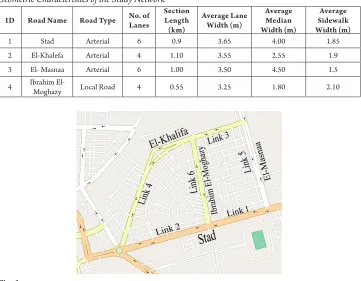
Table 1
Geometric Characteristics of the Study Network
ID Road Name Road Type No. of Lanes Section Length (km)
Average Lane Width (m)
Average Median Width (m)
Average Sidewalk Width (m)
1 Stad Arterial 6 0.9 3.65 4.00 1.85
2 El-Khalefa Arterial 4 1.10 3.55 2.55 1.9
3 El- Masnaa Arterial 6 1.00 3.50 4.50 1.5
4 Ibrahim El-Moghazy Local Road 4 0.55 3.25 1.80 2.10
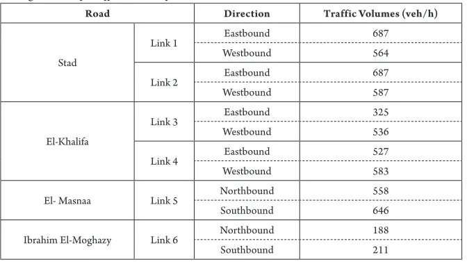
Fig. 1.
The Selected Network for the Study (From Google Maps)
3.2. Development of the Micro-simulation
Model
VISSIM is a microscopic simulation model that was developed by German company Planung Transport Verkher (PTV) Vision Suite. This software has the ability to simulate multimodal traffic flows including cars, trucks, buses, etc. VISSIM is versatile and provides the modeler with the ability to model a wide range of traffic operations in both the interrupted and uninterrupted traffic environment (PTV AG, 2014). VISSIM was chosen to simulate the study network where the behavior type was set to be urban traffic which uses Wiedemann
74 car following model. The following subsections provide more details on the model development.
3.2.1. Determination of Measures of
Effectiveness
3.2.2. Field Data Collection
Two types of data are required to build a VISSIM simulation model for the selected network. The first type of parameters includes existing geometric characteristics and traffic counts used for network coding of the simulation model. The second type is the field data used for the calibration/validation process of model parameters including average travel time and average travel speed.
Geometry Inputs
Geometry and network inputs include all other inputs to the model that are not associated with the volumes, traffic compositions, or routing decisions in VISSIM. The selected network was coded in VISSIM V. 7.00 using the data collected from the field. The simulator in the VISSIM model is responsible for generating traffic and is where the network is graphically built. Aerial photos were obtained from Google Maps patched together and used as a background for network coding.
Traffic Inputs
Volume data and traffic compositions were extracted at 15-minute intervals by manual classified counts on links of the selected network in the study area.
Traffic was classified into five vehicle classes: motorcycles, passenger cars including private cars and taxis, light good vehicles including mini trucks and microbuses, heavy vehicles and buses. Average travel speeds and average travel times were obtained using moving car technique for network links, in the study area.
Collection of traffic data was carried out in normal working days during the daylight hours. During data collection periods, the weather was clear and the pavement was dry. Average values of traffic volumes for the study network are presented in Table 2. Whereas average values of travel speeds and travel times for the study network are presented in Table 3.
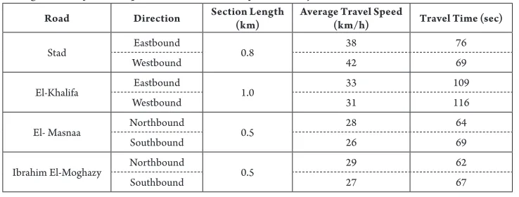
Table 2
Average Values of Traffic Volumes for the Network Links
Road Direction Traffic Volumes (veh/h)
Stad
Link 1 Eastbound 687
Westbound 564
Link 2 Eastbound 687
Westbound 587
El-Khalifa
Link 3 Eastbound 325
Westbound 536
Link 4 Eastbound 527
Westbound 583
El- Masnaa Link 5 Northbound 558
Southbound 646
Ibrahim El-Moghazy Link 6 Northbound 188
Table 3
Average Values of Travel Speeds and Travel Times for the Study Network
Road Direction Section Length (km) Average Travel Speed (km/h) Travel Time (sec)
Stad Eastbound 0.8 38 76
Westbound 42 69
El-Khalifa Eastbound 1.0 33 109
Westbound 31 116
El- Masnaa Northbound 0.5 28 64
Southbound 26 69
Ibrahim El-Moghazy Northbound 0.5 29 62
Southbound 27 67
3.2.3. Model Calibration
Model calibration is the process of modifying and determining the set of model parameters, based on modeling judgments and collected data. Such parameters accurately represent the prevailing field conditions of a given study area. In general, the target of calibration is to ensure that the simulation outputs of the evaluation variable match the observed data. Instead of calculating average errors to assess the quality of the calibration, a more robust approach is applied where the “matching” is evaluated using a suitable hypothesis statistical test. If the simulation output fits the observed data statistically then the model is said to be calibrated. Otherwise, the calibration variable would need further fine tuning (Manjunatha et al., 2013).
The desired speed distribution is one of the most influential parameters of a VISSIM simulation model. Therefore, average travel speed and traffic volume were chosen as the calibration parameters in the current analysis. The model would have been considered calibrated if a statistical agreement is found between the simulated and observed traffic volumes.
In this study, the evaluation criteria used in the calibration process includes:
- GEH Statistic
The GEH Statistic is a formula used in traffic engineering, traffic forecasting, and traffic modeling to compare observed versus simulated link volumes (Oketch and Carrick, 2005). The GEH formula gets its name from Geoffrey E. Havers, who invented it in the 1970s while working as a transport planner in London, England. The GEH is represented by the equation as below (Eq. (1)):
(1)
where: O = Observed hourly traffic volume values; and M = Simulated hourly traffic volume values.
Various GEH values give an indication of a goodness of fit, as outlined below:
GEH < 5: Traffic volumes can be considered a good fit;
5 < GEH < 10: Traffic volumes may require further investigation; and
- Coefficient of Determination (R2)
Coefficient of determination (R2) is a
statistical measure that gives information about the ‘goodness of fit’ of the model. In other words, it shows how well the regression line approximates the observed data points. If R2 = 1, the model is exactly predicting the
test data while R2 = 0 indicates there is no
correlation between the model results and the field measurements. However; a value of 0.75 or higher is recognized as good model (Xiong et al., 2014).
3.2.4. Model Validation
Validation of a simulation model is the next stage after ensuring that the model is well-calibrated. Validation is defined as the process of matching the output of the calibrated simulation model with some real-life measurements that were not used in the calibration. The evaluation measures used in this process should be different from the measures used in the calibration process. Alternatively, the measurements of the same variable can be utilized but for different locations, time periods, and/or traffic conditions (Park and Schneeberger, 2003). The model is deemed “valid” if the chosen MOE from the unused real-life dataset is close enough to the simulation values. Otherwise, the calibration process has to be re-executed until comparable results are achieved. Using travel time as MOE has been extensively reported in various studies. In this study, average travel times were selected as MOE for model validation. Average travel time was determined for all different vehicle classes for both the observed and the simulated travel times. The observed average travel times were computed using the collected data as described before.
In this study, the evaluation criteria used in the validation process include:
- Mean Absolute Percent Error (MAPE)
MAPE is a measure that used to calculate the average difference between simulated and observed data. The formula for the “MAPE” is (Eq. (2)):
(2)
- Root Mean Square Error (RMSE)
RMSE is a measure of average variation between observed and simulated data. It is often used to reflect the absolute deviation of data. The equation for calculating RMSE is shown below (Eq. (3)):
(3)
- Normalized Root Mean Square Error (RMSN)
RMSN is a measure of average variation between observed and simulated data. It is often used to indicate the relative deviation of data.
(4)
Where: O = Observed values; M = Simulated values; and N = Number of samples or observations.
The FHWA guide (FHWA, 2004) presented the evaluation criteria of the Wisconsin Department of Transportation (DOT) which generally suggest that a 15% error margin can be acceptable in similar exercises.
3.3. Traffic Management Measures
Various traffic management measures can be implemented to reduce air emissions due to road traffic. The following subsections describe the investigated measures in this study.
3.3.1. Improvement of Road Traffic Flow
Improvement of road traffic flow could reduce the number of traffic jams and thus reduce air emissions due to road traffic, because these emissions tend to increase at lower speeds and particularly with stop-start-driving (Cerezo, 1996). To study the effect of improvement of road traffic flow on air emissions, a new scenario was created using micro-simulation VISSIM software V. 7.00. The new scenario (Scenario 1) was created in the same network by increasing allowed road speed by 10 km/h hypothetically. This will be achieved by measures such as improving of road pavement condition and reducing number of side accesses.
3.3.2. Promotion of Public Transportation
Promotion of public transportation could decrease the use of private cars,
and thus reduce the congestion and the air emissions due to road traffic (Cerezo, 1996). To study the effect of promotion of public transportation on air emissions, a new scenario was created using micro-simulation VISSIM software V. 7.00. The new scenario (Scenario 2) was created in the same network with decreasing of traffic volumes by 10% hypothetically. It can be achieved by measures such as enhancing public transport services by increasing frequency, convenience and travel speed of public transport and setting restrictions for access to city centers for private and heavy traffic.
4. Results
4.1. Model Calibration
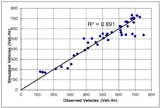
were accepted and model calibration was considered to be successfully completed. Also, coefficient of determination (R2) is
calculated to evaluate the accuracy of the model by indicating the correlation between field counts and simulated counts. The final
comparison of the observed and simulated traffic volumes is shown in Fig. 2, in which most of the comparison points conform to the diagonal line. Validation of the simulation model will be the final step to make sure that the model replicates field conditions for another measure.
Fig. 2.
Comparison of Observed and Simulated Counts for the Selected Network
Table 4
Results of GEH for Model Calibration
Road Direction
No
Calibration Criteria (GEH < Calibration 5) met?
After
Calibration Improvement (%)
GEH GEH
Stad
Link 1 WestboundEastbound 0.665.92 YesNo 0.540.94 18%84%
Link 2 WestboundEastbound 0.665.52 YesNo 0.541.07 18%81%
El-Khalifa
Link 3 WestboundEastbound 1.575.60 YesNo 1.564.82 14%1%
Link 4 WestboundEastbound 0.604.53 YesYes 0.604.37 0%4%
El- Masnaa Link 5 NorthboundSouthbound 3.796.32 YesNo 1.870.73 51%88%
Ibrahim El-Moghazy Link 6
Northbound 3.45 Yes 3.45 0%
4.2. Model Validation
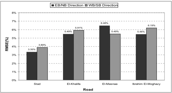
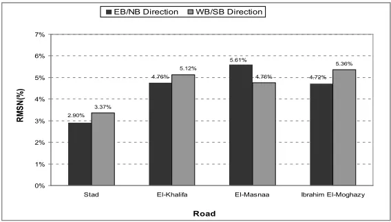
The simulated average travel times of the calibrated model were compared to the observed travel times. Different error measurements were computed for all vehicle classes and the results are presented in Fig. 3 to Fig. 5. From these figures, it can be
noticed that, all the error measurements were below 7% indicating a reasonable matching between the simulated and the observed travel times. Overall, all validation results were satisfactory with minimal errors. Therefore, it can be concluded that, the model is successfully calibrated and validated.
4.28%
2.65%
3.32%
4.27%
2.60%
4.62%
3.84% 4.92%
0% 1% 2% 3% 4% 5% 6%
Stad El-Khalifa El-Masnaa Ibrahim El-Moghazy
Road
MA
PE
(%
)
EB/NB Direction WB/SB Direction
Fig. 3.
Mean Absolute Percent Error Measurements for Model Validation of all Vehicle Classes for the Selected Network
3.35%
5.49%
6.48%
5.46%
3.89%
5.91%
5.49%
6.19%
0% 1% 2% 3% 4% 5% 6% 7% 8%
Stad El-Khalifa El-Masnaa Ibrahim El-Moghazy Road
RM
SE
(%
)
EB/NB Direction WB/SB Direction
Fig. 4.
4.76%
3.37%
4.76%
5.36%
2.90%
4.72% 5.61%
5.12%
0% 1% 2% 3% 4% 5% 6% 7%
Stad El-Khalifa El-Masnaa Ibrahim El-Moghazy
Road
RM
SN
(%
)
EB/NB Direction WB/SB Direction
Fig. 5.
Normalized Root Mean Square Error Measurements for Model Validation of all Vehicle Classes for the Selected Network
4.3. Simulation Analysis
Traffic simulation model is used to evaluate different scenarios, in terms of travel times, air emissions of CO, NOX and HC, and fuel
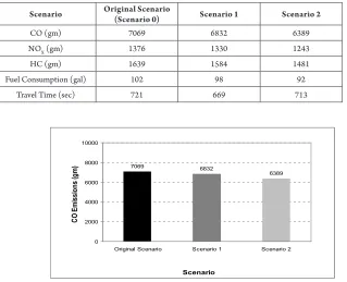
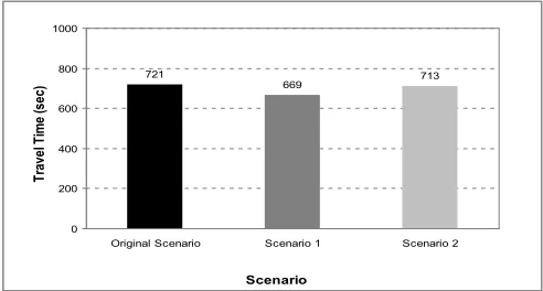
consumption. Such measures were collected as outputs from model simulation, in order to evaluate the effectiveness of each investigated traffic management scenario. The results of the 3600 sec (60 minutes) simulation period were used for the analysis. The results of total air emissions, fuel consumption and travel time aggregated on all network links for all scenarios are illustrated in Table 5. Also, the comparisons of different scenarios are shown in Fig. 6 to 10. These figures showed that;
• Increasing of road speed can reduce the emissions of CO, NOX and HC
and fuel consumption for all vehicle classes by about 3.35%. Also, there is a significant reduction in average travel time for all vehicle classes. The reduction rate of average travel time is about 7.21%.
• Decreasing of traffic volumes can reduce the emissions of CO, NOX and
HC and fuel consumption for all vehicle classes by about 9.61%. Also, there is no significant reduction in average travel time for all vehicle classes. The reduction rate of average travel time is about 1.10%.
Table 5
Total Air Emissions, Fuel Consumption and Travel Time Aggregated on all Network Links for Different Scenarios
Scenario Original Scenario (Scenario 0) Scenario 1 Scenario 2
CO (gm) 7069 6832 6389
NOX (gm) 1376 1330 1243
HC (gm) 1639 1584 1481
Fuel Consumption (gal) 102 98 92
Travel Time (sec) 721 669 713
7069 6832
6389
0 2000 4000 6000 8000 10000
Original Scenario Scenario 1 Scenario 2
Scenario
CO E
mis
sio
ns
(g
m)
Fig. 6.
Total CO Emissions Aggregated on all Network Links for Different Scenarios
1376 1330
1243
0 500 1000 1500 2000
Original Scenario Scenario 1 Scenario 2
Scenario
No
x E
m
issi
on
s (
gm
)
Fig. 7.
1639 1584
1481
0 500 1000 1500 2000
Original Scenario Scenario 1 Scenario 2
Scenario
HC
E
mi
ssi
on
s (
gm
)
Fig. 8.
Total HC Emissions Aggregated on all Network Links for Different Scenarios
102 98
92
0 30 60 90 120
Original Scenario Scenario 1 Scenario 2
Scenario
Fue
l C
ons
um
pt
ion (
ga
l)
Fig. 9.
Total Fuel Consumptions Aggregated on all Network Links for Different Scenarios
721
669 713
0 200 400 600 800 1000
Original Scenario Scenario 1 Scenario 2
Scenario
Tr
avel
T
im
e (
sec)
Fig. 10.
5. Conclusions and Recommendations
This paper investigates the impact of traffic management measures on air emissions due to road traffic. The micro-simulation model was developed for the selected network. Then, it calibrated and validated using the collected data. The model was calibrated using traffic volume and travel speed parameters and it was validated using travel time parameter. The study investigated three scenarios investigated using the developed model. The analysis was carried out using micro-simulation VISSIM software. Three major types of vehicle emissions were estimated; Carbon Monoxide (CO), Nitrogen Oxides (NOX) and Hydrocarbons (HC), also travel time and vehicle fuel consumption were estimated and aggregated on all network links for every scenario. Analysis showed that,
1. The superiority of the calibrated model compared to the model with default parameters in terms of improved GEH statistics.
2. Different error measurements were computed to assess the validity of the model. In general, all the errors were below 7% showing a reasonable matching between the observed and the simulated travel times.
3. The improvement of road traffic flow in the study network can reduce the emissions of CO, NOX and HC and fuel consumption for all vehicle classes by about 3.35%. Also, there is a significant reduction in average travel time for all vehicle classes. The reduction rate of average travel time is about 7.21%. 4. The promotion of public transportation
in the study network can reduce the emissions of CO, NOX and HC and fuel
consumption for all vehicle classes by about 9.61%. Also, there is no significant reduction in average travel time for all vehicle classes. The reduction rate of average travel time is about 1.10%. In summary, the improvement of road traffic flow in the study network can reduce air emissions as well as travel time whereas; the promotion of public transportation in the study network can reduce air emissions but cannot reduce travel time. Therefore the recommendations for practitioners may include improving road pavement condition, reducing number of side accesses, driving at a medium speed, well design of intersections, enhancing public transport services by increasing frequency, convenience and travel speed of public transport, and setting restrictions for access to city centers for private and heavy traffic.
A future extension of this work will include obtaining emissions field data in order to verify the results obtained from VISSIM using emissions detection instrument.
References
Balakrishna, R.; Antoniou, C.; Ben-Akiva, M.; Koutsopoulos, H.; Wen, Y. 2007. Calibration of Microscopic Traffic Simulation Models: Methods and Application, Transportation Research Record: Journal of the
Transportation Research Board (1999):198-207.
Cerezo, J. 1996. Traffic Management Strategies to Reduce Air Pollution, Transactions on the Built Environment 23: 141-147.
El Esawey, M; Sayed, T. 2011. Calibration and Validation of Simulation Models of Medium-Size Networks, Advances in Transportation Studies Section B (24): 57-76.
Environmental Protection Agency. 2005. Air Emission Sources. Available from internet: <http:// www.epa. gov/air/emissions/>.
FHWA. 2004. Traffic Analysis Toolbox, Volume III. Guidelines for Applying Traffic Micro-Simulation Modeling Software. Publication FHWA-HRT-04-040. Available from internet: <http://ops.fhwa.dot.gov/ trafficanalysistools/tat_vol3/index.htm />.
Jeihani, M.; James, P.; Saka, A.; Ardeshiri, A. 2015. Traffic Recovery Time Estimation under Different Flow Regimes in Traffic Simulation, Journal of Traffic and Transportation Engineering (English Edition) 2(5): 291-300.
Manjunatha, P.; Vortisch, P.; Mathew, T. 2013. Methodology for the Calibration of VISSIM in Mixed Traffic. In Proceedings of the Transportation Research Board, 92th Annual Meeting, 12 p.
Milam, R., 2000. Recommended Guidelines for the Calibration and Validation of Traffic Simulation Models. Available from internet: <http:/www.fehrandpeers. com/>.
Neunhauserer, L.; Diegmann, V. 2010. Analysis of the Impacts of an Environmental Traffic Management System on Vehicle Emissions and Air Quality. In Proceedings of the 18th International Symposium Transport and Air Pollution (TAP’10), 6 p.
Oketch, T.; Carrick, M. 2005. Calibration and validation of a micro-simulation model in network analysis. In Proceedings of the Transportation Research Board, 84th Annual Meeting, 17 p.
Olarte, C. 2011. Operational and Environmental Comparisons between Left-turn Bypass, Diverging Flow and Displaced Left-turn Intersection Designs, Master Degree thesis, College of Engineering and Computer Science, Florida Atlantic University, USA.
Park, B.; Schneeberger, J.D. 2003. Microscopic Simulation Model Calibration and Validation: Case Study of Vissim Simulation Model for a Coordinated Actuated Signal System, Transportation Research Record, Journal of the Transportation Research Board 1856: 185-192.
PTV AG. 2014. VISSIM 7.00 User Manual. PTV Plannung Transport Verkehr AG. Karlsruhe. Germany.
Rakha, H.; Van Aerde, M.; Ahn, K.; Trani, A. 2000. Requirements for Evaluating Traffic Signal Control Impacts on Energy and Emissions Based on Instantaneous Speed and Acceleration Measurements, Transportation Research Record: Journal of the Transportation
Research Board 1738: 56-67.
Srinivasan, R.; Subramaniam, S. 1979. Automobile and Air Pollution, Indian Highways. In Proceedings of the Indian Roads Congress, 7(12): 27-39.
Xiong, C.; Zhu, Z.; He, X.; Chen, X.; Zhu, S.; Mahapatra, S.; Chang, G.L.; Zhang, L. 2015. Developing a 24-hour Large-scale Microscopic Traffic Simulation Model for the Before and-After Study of a New Tolled Freeway in the Washington Dc-Baltimore Region. In Proceedings of the Transportation Research Board, 93th Annual Meeting, 20 p.
Zallinger, M.; Luz, R.; Hausberger, S.; Hirschmann, K.; Fellendorf, M. 2010. Coupling of Microscale Traffic and Emission Models to Minimize Emissions by Traffic Control Systems. In Proceedings of the 18th International