A SURVEY ON FEATURE SELECTION
TO PERFORM CLASSIFICATION USING
META HEURISTIC ALGORITHMS IN
DATA MINING DOMAIN
Dr. SANTHI BASKARAN
Professor, Department of Information Technology Pondicherry Engineering College, Puducherry, India
V. YASASWINI
Research ScholarDepartment of Computer Science & Engineering Pondicherry Engineering College, Puducherry, India
Abstract
Feature selection becomes the focus of much research in many areas of applications for which datasets with large number of features are available. Feature Selection Methods in Data mining and Data analysis problems aim at selecting a subset of the features that describe the data in order to get a compact and exact representation of the available information hidden in the data. The selected subset of data is the most useful and contains all the useful information with all the irrelevant data is deleted. The dimensionality of the feature space when being high affects the classification accuracies and the computational complexity due to redundant, irrelevant and noisy features present in the dataset. The role of feature selection is in the context of deep learning and how feature selection is related to feature engineering. Relevant feature identification has become an essential task to apply data mining algorithms effectively in real-world scenarios. Therefore, many feature selection methods have been proposed to obtain the relevant feature or feature subsets in the literature to achieve objectives of classification and clustering. A comprehensive overview, categorization, and comparison of existing feature selection methods
are also done, and the guidelines are also provided to select a feature selection algorithm without knowing the information of each algorithm. Classification is a data mining (machine learning) technique used to predict group membership for data instances. Several major kinds of classification method include decision tree induction, Bayesian networks, k-nearest neighbor classifier, case-based reasoning, genetic algorithm and fuzzy logic techniques. The goal of this survey is to find the best feature selection method and classification technique to demonstrate the use of feature selection using classification in data mining. We conclude this work by identifying trends and challenges of feature selection research and development.
Keywords- Bayesian, Classification, Classification technique, Clustering, Data mining, Evaluation, Feature Selection, fuzzy logic, Relevance.
I.INTRODUCTION
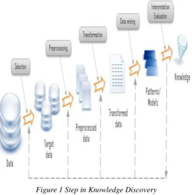
for discovering previously unknown, valid patterns and relationships in huge data set. Data mining consists of more than collection and managing the data, it also includes analysis and prediction. Data mining (the advanced analysis step of the "Knowledge Discovery in Databases" process, or KDD) an interdisciplinary subfield of computer science, is the computational process of discovering patterns in large data sets involving methods at the intersection of artificial intelligence, machine learning, statistics, and database systems. The overall goal of the data mining process is to extract information from a data set and transform it into an understandable structure for further use. Aside from the raw analysis step, it involves database and data management aspects, data preprocessing, model and inference considerations, interestingness metrics, complexity considerations, post-processing of discovered structures, visualization and online updating.
Figure 1 Step in Knowledge Discovery
Process of Data Mining
While large-scale information technology has been evolving separate transaction and analytical systems, data mining provides the link between the two. Data mining software analyzes relationships and patterns in stored transaction data based on open-ended user queries. Several types of analytical software are available: statistical,
machine learning, and neural networks. Generally, any of four types of relationships are sought: Classes: Stored data is used to locate data in
predetermined groups. For example, a restaurant chain could mine customer purchase data to determine when customers visit and what they typically order. This information could be used to increase traffic by having daily specials.
Clusters: Data items are grouped according to
logical relationships or consumer preferences. For example, data can be mined to identify market segments or consumer affinities. Associations: Data can be mined to identify
associations. The beer-diaper example is an example of associative mining.
Sequential patterns: Data is mined to anticipate
behavior patterns and trends. For example, an outdoor equipment retailer could predict the likelihood of a backpack being purchased based on a consumer's purchase of sleeping bags and hiking shoes.
Feature Selection in Data Mining
Feature selection (FS) [1] is a term commonly used in data mining to describe the tools and techniques available for reducing inputs to a manageable size for processing and analysis. FS implies not only cardinality reduction, which means imposing an arbitrary or predefined cutoff on the number of attributes that can be considered when building a model, but also the choice of attributes, meaning that either the analyst or the modeling tool actively selects or discards attributes based on their usefulness for analysis.
of the columns is very sparse you would gain very little benefit from adding them to the model. If you keep the unneeded columns while building the model, more CPU and memory are required during the training process, and more storage space is required for the completed model.
Even if resources are not an issue, you typically want to remove unneeded columns because they might degrade the quality of discovered patterns, for the following reasons: Some columns are noisy or redundant. This
noise makes it more difficult to discover meaningful patterns from the data;
To discover quality patterns, most data mining
algorithms require much larger training data set on high-dimensional data set. But the training data is very small in some data mining applications.
If only 50 of the 500 columns in the data source have information that is useful in building a model, you could just leave them out of the model, or you could use FS techniques to automatically discover the best features and to exclude values that are statistically insignificant. FS helps solve the twin problems of having too much data that is of little value, or having too little data that is of high value.
Figure 2. Characterization of Feature Selection
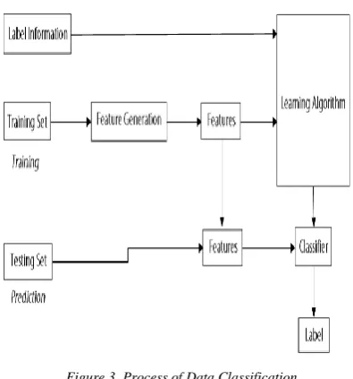
Classification System
In machine learning and pattern recognition, classification refers to an algorithmic procedure for assigning a given piece of input data into one of a given number of categories [1]. An example would be assigning a given email into
"spam" or "non-spam" classes or assigning a diagnosis to a given patient as described by observed characteristics of the patient (gender, blood pressure, presence or absence of certain symptoms, etc). An algorithm that implements classification, especially in a concrete implementation, is known as a classifier. The term "classifier" sometimes also refers to the mathematical function, implemented by a classification algorithm that maps input data to a category.
The piece of input data is formally termed an instance, and the categories are termed classes. The instance is formally described by a vector of features, which together constitute a description of all known characteristics of the instance. Typically, features are either categorical (also known as nominal, i.e. consisting of one of a set of unordered items, such as a gender of "male" or "female", or a blood type of "A", "B", "AB" or "O"), ordinal (consisting of one of a set of ordered items, e.g. "large", "medium" or "small"), integer-valued (e.g. a count of the number of occurrences of a particular word in an email) or real-valued (e.g. a measurement of blood pressure). Often, categorical and ordinal data are grouped together; likewise for integer-valued and real-valued data. Furthermore, many algorithms work only in terms of categorical data and require that real-valued or integer-valued data be separated into groups (e.g. less than 5, between 5 and 10, or greater than 10).
the distance between instances, considered as vectors in a multi-dimensional vector space).
Classification and clustering are examples of the more general problem of pattern recognition, which is the assignment of some sort of output value to a given input value. Other examples are regression, which assigns a real-valued output to each input; sequence labeling, which assigns a class to each member of a sequence of values (for example, part of speech tagging, which assigns a part of speech to each word in an input sentence); parsing, which assigns a parse tree to an input sentence, describing the syntactic structure of the sentence; etc.
Figure 3. Process of Data Classification
Classification Techniques in Data Mining
Classification technique [4] is capable of processing a wider variety of data than regression and is growing in popularity. There are several applications for Machine Learning (ML), the most significant of which is data mining. People are often prone to making mistakes during analysis or, possibly, when trying to establish relationships between multiple features. This makes it difficult for them to find solutions to certain problems. Machine learning can often be successfully applied to these problems, improving the efficiency of systems and the designs of machines. There are
techniques likes Decision Tree Induction, Bayesian Network, K-Nearest Neighbor.
Decision Tree Induction
Decision trees are trees that classify instances by sorting them based on feature values. Each node in a decision tree represents a feature in an instance to be classified, and each branch represents a value that the node can assume. Instances are classified starting at the root node and sorted based on their feature values.
The basic algorithm for decision tree induction is a greedy algorithm that constructs decision trees in a top-down recursive divide-and-conquer manner. The algorithm is summarized as follows.
Create a node N;
If samples are all of the same class, C then return N as a leaf node labeled with the class
C;
If attribute-list is empty then
return N as a leaf node labeled with the most
common class in samples;
Select test-attribute, the attribute among
attribute-list with the highest information gain; Label node N with test-attribute;
for each known value ai of test-attribute Grow a branch from node N for the condition
test-attribute= ai;
let si be the set of samples for which
test-attribute= ai; if si is empty then
attach a leaf labeled with the most common
class in samples;
else attach the node returned by
Generate_decision_tree (si,attribute-list_test-attribute)
belonging to a specific class. Since a decision tree constitutes a hierarchy of tests, an unknown feature value during classification is usually dealt with by passing the example down all branches of the node where the unknown feature value was detected, and each branch outputs a class distribution. The output is a combination of the different class distributions that sum to 1. The assumption made in the decision trees is that instances belonging to different classes have different values in at least one of their features. Decision trees tend to perform better when dealing with discrete/categorical features. Bayesian Networks
Bayesian Network (BN) is a graphical model for probability relationships among a set of variables features. The Bayesian network structure S is a directed acyclic graph (DAG) and the nodes in S are in one-to-one correspondence with the features X. The arcs represent casual influences among the features while the lack of possible arcs in S encodes conditional independencies. Moreover, a feature (node) is conditionally independent from its non-descendants given its parents (X1 is conditionally independent from X2 given X3 if P (X1|X2, X3) = P (X1|X3) for all possible values of X1, X2, X3). Typically, the task of learning a Bayesian network can be divided into two subtasks: initially, the learning of the DAG structure of the network, and then the determination of its parameters. Probabilistic parameters are encoded into a set of tables, one for each variable, in the form of local conditional distributions of a variable given its parents. Given the independences encoded into the network, the joint distribution can be reconstructed by simply multiplying these tables.
The structure of a Bayesian network can take the following forms:
Declaring that a node is a root node, i.e., it has
no parents.
Declaring that a node is a leaf node, i.e., it has
no children.
Declaring that a node is a direct cause or direct
effect of another node.
Declaring that a node is not directly connected
to another node.
Declaring that two nodes are independent,
given a condition-set.
Providing partial nodes ordering, that is,
declare that a node appears earlier than another node in the ordering.
Providing a complete node ordering.
Figure 4.Structure of Bayes Network
A problem of BN classifiers is that they are not suitable for datasets with many features. The reason for this is that trying to construct a very large network is simply not feasible in terms of time and space. A final problem is that before the induction, the numerical features need to be discredited in most cases.
K-Nearest Neighbor Algorithm
Nearest neighbor classifiers are based on learning by analogy. The training samples are described by n dimensional numeric attributes. Each sample represents a point in an n-dimensional space. In this way, all of the training samples are stored in an n-dimensional pattern space. When given an unknown sample, a k-nearest neighbor classifier searches the pattern space for the k training samples that are closest to the unknown sample. "Closeness" is defined in terms of Euclidean distance, where the Euclidean distance between two points, X=(x1,x2,……,xn) and
d(X,Y) = 𝑛𝑖=1 𝑥𝑖− 𝑦𝑖 2
The unknown sample is assigned the most common class among its k nearest neighbors. When k=1, the unknown sample is assigned the class of the training sample that is closest to it in pattern space.
Nearest neighbor classifiers are instance-based or lazy learners in that they store all of the training samples and do not build a classifier until a new (unlabeled) sample needs to be classified. This contrasts with eager learning methods, such as a decision tree induction and back propagation, which constructs a generalization model before receiving new samples to classify. Lazy learners can incur expensive computational costs when the number of potential neighbors (i.e., stored training samples) with which to compare a given unlabeled sample is great. Therefore, they require efficient indexing techniques. An expected lazy learning method is faster at training than eager methods, but slower at classification since all computation is delayed to that time. Unlike decision tree induction and back propagation, nearest neighbor classifiers assign equal weight to each attribute. This may cause confusion when there are many irrelevant attributes in the data. Nearest neighbor classifiers can also be used for prediction, that is, to return a real-valued prediction for a given unknown sample. In this case, the classifier returns the average value of the real-valued prediction associated with the k nearest neighbors of the unknown sample. The k-nearest neighbors’ algorithm is amongst the simplest of all machine learning algorithms. An object is classified by a majority vote of its neighbors, with the object being assigned to the class most common amongst its k nearest neighbors. k is a positive integer, typically small.
If k = 1, then the object is simply assigned to the class of its nearest neighbor. In binary (two class) classification problems, it is helpful to
choose k to be an odd number as this avoids tied votes. The same method can be used for regression, by simply assigning the property value for the object to be the average of the values of its k nearest neighbors. It can be useful to weigh the contributions of the neighbors, so that the nearer neighbors contribute more to the average than the more distant ones.
The neighbors are taken from a set of objects for which the correct classification (or, in the case of regression, the value of the property) is known. This can be thought of as the training set for the algorithm, though no explicit training step is required. In order to identify neighbors, the objects are represented by position vectors in a multidimensional feature space. It is usual to use the Euclidian distance, though other distance measures, such as the Manhattan distance could in principle be used instead. The k-nearest neighbor algorithm is sensitive to the local structure of the data.
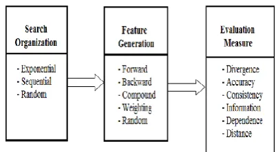
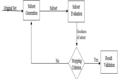
Procedure of Feature Selection
process of subset generation and evaluation is repeated until a given stopping criterion is satisfied. Then, the selected best subset usually needs to be validated by prior knowledge or different tests via synthetic and/or real world data sets. Feature selection can be found in many areas of data mining such as classification, clustering, association rules, and regression. For example, feature selection is called subset or variable selection in Statistics. A number of approaches to variable selection and coefficient shrinkage for regression are summarized. In this survey, we focus on feature selection algorithms for classification and clustering. Early research efforts mainly focus on feature selection for classification with labeled data (supervised feature selection) where class information is available. Latest developments, however, show that the above general procedure can be well adopted to feature selection for clustering with unlabeled data (or unsupervised feature selection) where data is unlabeled.
Figure 5. Four steps of Feature Selection
Comparison of Feature Selection
There exists a vast body of available feature selection algorithms. In order to better understand the inner instrument of each algorithm along with commonalities and differences among them, we explained the different feature selection algorithms which are categorized into Filter, Wrapper, and Hybrid based on selection criteria [19]. Each algorithm has its own strength and weakness. Table 1 compares some of the available algorithms. Filter Method selects the feature subset on the basis of intrinsic characteristics of the data, independent of mining algorithm. It can be applied to data with high dimensionality. The advantages of Filter method are its generality and high computation efficiency.
Wrapper Method requires a predetermined algorithm to determine the best feature subset. Predictive accuracy of the algorithm is used for evaluation. This method guarantees better results, but it is computationally expensive for large dataset. For this reason, the Wrapper method is not usually preferred.
Hybrid Method combines Filter and Wrapper to achieve the advantages of both the methods. It uses an independent measure and a mining algorithm to measure the goodness of newly generated subset. In this approach, Filter method is first applied to reduce the search space and then a wrapper model is applied to obtain the best feature subset.
Algorithm Type Factors/Approaches used Benefit Drawback
Relief Filter Relevance Evaluation
It is scalable to data set with increasing dimensionality.
It cannot eliminate the redundant features.
Correlation- based Feature Selection
Filter
Uses Symmetric Uncertainty (for calculating Feature-
Class and Feature-Feature correlation)
It handles both irrelevant and redundant features and It prevents the reintroduction
Of redundant
features.
It works well on smaller datasets It cannot handle
Algorithm Type Factors/Approaches used Benefit Drawback
Fast Correlation Based Filter
Filter
uses predominant correlation as a goodness measure, based on symmetric Uncertainty (SU). It hugely reduce
It hugely reduce the dimensionality
It cannot handle feature
redundancy.
Interact Filter
Uses symmetric uncertainty and Backward Elimination
Approach
It improves the accuracy.
Its mining
performance
decreases, as the dimensionality increases. Fast
Clustering-Based
Feature Subset Selection
Filter
Graph-Theoretic Clustering Method used for clustering and a best feature is chosen from each cluster.
Dimensionality is hugely reduced
Works well only for Microarray data. Condition Dynamic Mutual Information Feature Selection
Filter Mutual Information
Better Performance
in Mutual
Information
Sensitive to noise
Affinity Propagation – Sequential Feature Selection Wrapper
Affinity Propagation clustering algorithm
applied to get the clusters
SFS applied for each cluster to get the best subset
Faster than
Sequential Feature Selection
Accuracy is not better than SFS
Evolutionary Local Selection Algorithm
Wrapper K-Means Algorithm used for clustering
Covers a large space of possible feature combinations
As the number of features increases, the cluster quality decreases.
Wrapper Based Feature Selection using SVM
Wrapper Sequential Forward Selection for feature selection
Better Accuracy and Faster Computation
Hybrid Feature
Selection Hybrid
(Filter) Mutual Information (Wrapper)Wrapper model based feature selection algorithm
Improves Accuracy
High Computation Cost for high dimensional data set
Two-Phase Feature Selection Approach
Hybrid
(Filter) Artificial Neural Network Weight Analysis used to remove irrelevant features.
(Wrapper) Genetic Algorithm used to remove redundant features
Handles both
irrelevant and Redundant features. Improves Accuracy
Table 1. Categorization of Feature Selection Algorithms.
Experiments and Result
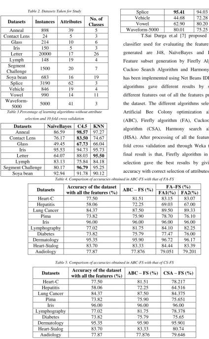
Fourteen standard datasets drawn from the UCI collection proposed by B.Kalpana et.al [6] were used in the experiments. These datasets were chosen due to nominal class features. The number of instances, attributes and number of classes vary in the chosen dataset to represent different combinations. The learning algorithm chosen for classifying are Naïve Bayes, K-NN (k=10) and C4.5 tree. All datasets were run on Pentium
Table 2. Datasets Taken for Study
Datasets Instances Attributes No. of Classes
Anneal 898 39 5
Contact Lens 24 5 3
Glass 214 10 6
Iris 150 5 3
Letter 20000 17 26
Lymph 148 19 4
Segment
Challenge 1500 20 7
Soya bean 683 16 19
Splice 3190 62 3
Vehicle 846 19 4
Vowel 990 14 11
Waveform-5000 5000 41 3
Table 3.Percentage of learning algorithms-without attribute
selection and 10 fold cross validation
Datasets NaïveBayes C4.5 KNN
Anneal 86.59 98.57 97.27
Contact Lens 76.17 83.50 74.67
Glass 49.45 67.73 66.04
Iris 95.53 94.73 95.73
Letter 64.07 88.03 95.50
Lymph 83.13 75.84 84.18
Segment Challenge 80.17 96.79 95.25
Soya bean 92.94 91.78 90.12
Splice 95.41 94.03 79.86
Vehicle 44.68 72.28 70.17
Vowel 62.90 80.20 93.39
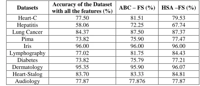
Waveform-5000 80.01 75.25 79.29 T.Sai Durga et.al [7] proposed that the classifier used for evaluating the feature subsets generated are J48, NaïveBayes and Logistic. Feature subset generation by Firefly Algorithm, Cuckoo Search Algorithm and Harmony Search has been implemented using Net Beans IDE. These algorithms gave different results by selecting different features out of all the features present in the dataset. The different algorithms selected are Artificial Bee Colony optimization algorithm (ABC), Firefly algorithm (FA), Cuckoo search algorithm (CSA), Harmony search algorithm (HSA). After processing of all the features in 10 fold cross validation and through Weka tool, the final result is that, Firefly algorithm in Feature selection gave the best results by giving best accuracy with correct selection of attributes. Table 4. Comparison of accuracies obtained in ABC-FS with that of FA-FS
Datasets Accuracy of the dataset
with all the features (%) ABC – FS (%)
FA–FS (%) FA1(%) FA2(%)
Heart-C 77.50 81.51 83.15 83.07
Hepatitis 58.06 72.25 69.03 67.00
Lung Cancer 84.37 87.50 89.50 89.33
Pima 73.82 75.90 78.70 76.10
Iris 96.00 96.00 96.00 96.00
Lymphography 77.02 81.75 84.10 82.25
Diabetes 73.82 75.79 77.47 76.00
Dermatology 95.35 95.90 96.72 96.17
Heart-Stalog 83.70 83.33 84.44 83.39
Audiology 77.87 77.876 79.051 79.201
Table 5. Comparison of accuracies obtained in ABC-FS with that of CS-FS
Datasets Accuracy of the dataset
with all the features (%) ABC – FS (%) CSA – FS (%)
Heart-C 77.50 81.51 78.217
Hepatitis 58.06 72.25 64.516
Lung Cancer 84.37 87.50 84.375
Pima 73.82 75.90 75.651
Iris 96.00 96.00 96.00
Lymphography 77.02 81.75 78.378
Diabetes 73.82 75.79 75.65
Dermatology 95.35 95.90 95.901
Heart-Stalog 83.70 83.33 80.74
Table 6. Comparison of accuracies obtained in ABC-FS with that of HSA-FS
Datasets Accuracy of the Dataset
with all the features (%) ABC – FS (%) HSA –FS (%)
Heart-C 77.50 81.51 79.53
Hepatitis 58.06 72.25 67.74
Lung Cancer 84.37 87.50 87.37
Pima 73.82 75.90 77.47
Iris 96.00 96.00 96.00
Lymphography 77.02 81.75 84.43
Diabetes 73.82 75.79 77.21
Dermatology 95.35 95.90 96.07
Heart-Stalog 83.70 83.33 84.81
Audiology 77.87 77.876 77.87
Thair Nu Phyu [8] proposed different Classification Techniques in data mining. Decision trees and Bayesian Network (BN) generally have different operational profiles, when one is very accurate the other is not and vice versa. On the contrary, decision trees and rule classifiers have a similar operational profile. The goal of classification result integration algorithms is to generate more certain, precise and accurate system results. Numerous methods have been suggested for the creation of ensemble of classifiers. Although or perhaps because many methods of ensemble creation have been proposed, there is as yet no clear picture of which method is best. Classification methods are typically strong in modeling interactions. Several of the classification methods produce a set of interacting loci that best predict the phenotype. However, a straightforward application of classification methods to large numbers of markers has a potential risk, picking up randomly associated markers.
Samina Khalid et.al [13], proposed comparison of Feature Selection Algorithms and extraction. The objective of both selection and extraction methods concerns the reduction of feature space in order to improve data analysis. This aspect becomes more important when real world datasets are considered, which can contain hundreds or thousands features. The main difference between feature selection and extraction is that the first performs the reduction by selecting
a subset of features without transforming them, while feature extraction reduces dimensionality by computing a transformation of the original features to create other features that should be more significant. Traditional methods and their recent enhancements as well as some interesting applications concerning feature selection are presented. Feature selection improves knowledge of the process under consideration, as it points out the features that mostly affect the considered phenomenon. Moreover the computation time of the adopted learning machine and its accuracy need to be considered as they are crucial in machine and data mining applications.
II.CONCLUSION
survey concludes that feature selection gives better results than feature extraction. We propose to use the best Feature Selection method to perform Classification for UCI dataset to get results with best accuracy through minimum number of attributes.
Now-a-days there is a huge amount of production data and people want to get the necessary information in real time environment, which requires us to learn and adapt our technologies and techniques. Provided this, it was interesting to explore these increasingly dominant options in the world of technology.
III.REFERENCES
1) Jiliang Tang, Salem Alelyani and Huan Liu. Feature Selection for Classification: A Review. 2) Q. Gu, Z. Li, and J. Han. Towards feature
selection in network. In International Conference on Information and Knowledge Management, 2011.
3) A.Frank, A. Asuncion, UCI Machine Learning Repository, (http://archive.ics.uci.edu/ml. Irvine, CA: University of
4) California, School of Information and Computer Science (2010))
5) Han, J., and Kamber. M.: Data mining concepts and techniques. Academic Press, 2001.
6) Huan liu and lei yu. Toward integrating Feature Selection algorithms for Classification and Clustering. IEEE transactions on Knowledge and Data Engineering, vol 17. No 4, April 2005.
7) B.Kalpana, Dr.V.Saravanan and Dr. K. Vivekanandan. A survey of feature Selection models on Classification. Vol 3, No.1, Jan-Feb, 2012.
8) T.Sai Durga, V.Yasaswini. An Enhancement for the optimization of feature selection to perform Classification Using Meta Heuristic
Algorithms. In International Journal of Latest Engineering Research and Applications (IJLERA), Volume – 01, Issue – 09, December – 2016, PP – 64-70.
9) Tu, C.J., Chuang, L., Chang, J. and Yang, C. (2007). Feature Selection using PSO-SVM. IAENG International Journal of Computer Science, Vol. 33, No. 1, pp. 18 – 23.
10) Thair Nu Phyu. Survey of Classification Techniques in Data Mining. International Multi Conference of Engineers and Computer Scientists 2009 Vol I IMECS 2009, March 18 - 20, 2009, Hong Kong.
11) N.Suguna and K.G.Thanushkodi. An Independent Rough Set Approach Hybrid with Artificial Bee Colony Algorithm for Dimensionality Reduction. American Journal of Applied Sciences 8 (3): 261 – 266, 2011. 12) Jianyu Mia and Lingfeng Niu. A Survey on
Feature Selection. Procedia Computer Science 91 (2016) 919 – 926
13) Pradnya Kumbhar, Manisha Mal . A Survey on Feature Selection Techniques & Classification Algorithms for Efficient Text Classification. Index Copernicus Value (2013),2319-7064. 14) Samina Khalid, Tehmina Khalil, Shamila
Nasreen. A Survey of Feature Selection and Feature Extraction Techniques in Machine Learning. Science and Information Conference 2014, August 27-29, 2014.
15) I. Guyon and A. Elisseeff. An Introduction to Variable and Feature Selection. Journal of Machine Learning Research, vol.3, pp. 1157- 1182, 2003.
17) N. Elavarasan, Dr. K.Mani. A Survey on Feature Extraction Techniques.Vol. 3, Issue 1, January 2015.
18) Jun Wang, Jin-Mao Wei, Zhenglu Yang, and Shu-Qin Wang. Feature Selection by Maximizing Independent Classification Information, IEEE Transactions on Knowledge and Data Engineering 2016
19) Ricardo Bragança, Filipe Portela, A. Vale, Tiago Guimaraes, and Manuel Santos. Data Mining Classification Models for Industrial Planning. ICACDS 2016, CCIS 721, pp. 585–594, 2017.
20) K.Sutha, Dr.J. Jebamalar Tamilselvi. A Review of Feature Selection Algorithms for Data Mining Techniques. International Journal on Computer Science and Engineering (IJCSE). ISSN: 0975-3397 Vol. 7 No.6 Jun 2015.