GLOBAL JOURNAL OF ADVANCED ENGINEERING TECHNOLOGIES AND
SCIENCES
CHARACTERIZATION OF A HYDRAULIC SYSTEM WITH MULTIPLE
EXHAUSTS
Luiz Gustavo Martins Vieira*, Vitor Alves Garcia, Danylo Oliveira Silva
*Chemical Engineering School, Federal University of Uberlândia, Uberlândia, Brazil
ABSTRACT
Hydraulic systems are traditionally constituted by one suction and one exhaust connected by pipes. Between the suction and the exhaust, pumps and many devices can be placed (reduction, expansion, valves, equipment, etc.). Hydraulic projects usually consist in predicting the fluid volumetric flow rate (volumetric capacity) that can flow through the hydraulic system according to its main features: piping size (diameter and length), kind of accessories, pump power, inlet and outlet pressure conditions, and the elevation of the suction and exhaust. However, this study investigated the behavior of a hydraulic system with the addition of multiple exhaust lines just after the pump, connected to a distributor. In this case, predicting the volumetric capacity of a hydraulic system was more complex, because the new fluid flow rate must be distributed according to the characteristics of each exhaust. Mathematically, a set of nonlinear equations was established based on the fundamentals of Fluid Mechanics and it was solved simultaneously. This methodology predicted the volumetric capacity according to the number of attached piping lines and other features of the hydraulic system, such as length, diameter, roughness, elevation, and pump power. Experimental validations demonstrated that the deviations of the numerical method adopted in this study were lower than 4%. The addition of multiple exhausts was beneficial because it considerably increased the volumetric capacity for the same pump power installed. As an example, when the number of exhausts changed from 2 to 4, from 4 to 6, and from 6 to 8, the volumetric capacity of the experimental system increased in 86%, 45%, and 24%, respectively. This study also indicated the variables that most affected the volumetric capacity: the piping diameter, the elevation of the exhausts, and the amount of exhausts, in this order.
KEYWORDS: Volumetric capacity; Distributor; Pump power; Energy cost.
INTRODUCTION
The Bernoulli Equation has many applications in Fluid Mechanics because it helps predict the volumetric capacity of a hydraulic system or the necessary power to pump a given fluid [1-3]. In its original conception, the Bernoulli Equation is an algebraic equation [Eq. (1)]. It is a simplification of the Equation of Motion [4] for special physical conditions, such as steady-state flow, ideal (negligible viscous effects) and incompressible flow, absence of heat exchange and shaft work with the surroundings, and macroscopic flow in a preferential direction.
2 2
1 1 2 2
1 2
P v P v
z z
g 2g g 2g
(1)In the ideal conditions of Eq. (1), the user would only have to know the operating conditions (P, v, z) at the start (1) and at the end (2) of the flow to provide a generalized physical description of fluid dynamics. However, in real flows, Eq. (1) must be rewritten considering head losses (hC), due to viscous dissipation in the pipes and accessories, and also the pump (hP) and turbine heads (hT) eventually inserted in the hydraulic system [5]. In these hypotheses, Bernoulli Equation must be rewritten as Eq. (2).
2 2
1 1 2 2
1 P 2 C T
P v P v
z h z h h
g 2g g 2g
(2)In practice, turbine (hT) and pump heads (hP) are well known information provided by their manufacturers, then it is not difficult to find them out. In turn, the evaluation of head loss (distributed or localized) depends on adequate empirical coefficients and equations, which are usually provided by the literature [6]. The Bernoulli Equation [Eq. (2)] is often applied when the fluid mass remains the same during the flow, since there is only one inlet (suction) and one outlet (exhaust) in most of the systems analyzed [7]. In these conditions, the algebraic manipulation of Bernoulli Equation is perfectly feasible, without major problems to predict any of its terms.
Therefore, due to the addition or division of the mass flow rate, the number of equations and the mathematical effort to solve them will certainly increase [9-12].
This study aimed to verify the effect of multiple exhausts on the volumetric flow rate of a given hydraulic system. For that reason, the number of exhausts was combined with other relevant factors for the fluid flow in a hydraulic system (length, diameter, elevation, roughness, pump power) in the form of a Central Composite Design (CCD). Numerical and experimental studies were carried out to validate the methodology adopted in this research and to quantify the effects of each variable on the volumetric capacity of a hydraulic system.
METHODOLOGY
Setting out Physical-Mathematical Equations for a Hydraulic System with Multiple Exhausts
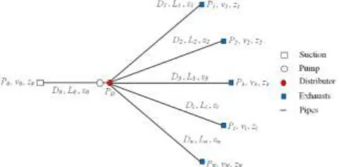
Figure 1 provides a schematic, generic representation of a hydraulic system consisted of a suction, a pump, a distributor, and N exhausts.
Figure 1: Schematic representation of a hydraulic system with multiple exhausts
One of the hypothesis in this methodology was to consider the dimensions of the distributor as finite so that the fluid pressure is almost constant in the whole volume of this accessory ( P 0).
Thus, a Bernoulli Equation was established from the suction to the distributor (first line of the matrix of Eq. (3)) and N Bernoulli equations for each outlet from the distributor to its respective exhaust. For each N+1 Bernoulli Equation established [Eq. (3)], other (N+1) equations must be also set out to estimate the friction coefficients [Eq. (4)] according to the Colebrook-White Equation.
2
0 D 0 0
0 P D 0 S 0
0 2
D 1 1 1
D 1 1 S 1
1
2
D 2 2 2
D 2 2 S 2
2
2
i i i
D
D i i S i
i
2
N N N
D
D N N S N
N
P P L v
z h z f K
g g D 2g
P P L v
z z f K
g g D 2g
P P L v
z z f K
g g D 2g
P L v
P
z z f K
g g D 2g
P L v
P
z z f K
g g D 2g
0 0
0 0 0
1 1
1 1 1
2 2
2 2 2
i i
i i i
N N
N N N
D
1 2.5
2 log 3.7
f Re f
D
1 2.5
2 log 3.7
f Re f
D
1 2.5
2 log 3.7
f Re f
D
1 2.5
2 log 3.7
f Re f
D
1 2.5
2 log 3.7
f Re f
0 0 0 0 0 (4)
The matrices represented by Eq. (3) and (4) account for 2(N+1) nonlinear equations. If all other conditions are well known for the hydraulic system (fluid, diameter, length, roughness, elevation, pump power output, suction pressure, exhaust pressure and loss coefficients), the terms to be calculated would be N+1 average velocities (v0, v1, v2, ..., vi, ...,
vN), N+1 friction factors (f0, f1, f2, ..., fi, ..., fN), and the absolute pressure in the distributor (PD). Therefore, the number of unknowns [2(N+1)+1] would be higher than the number of available equations [2(N+1)], which does not allow to immediately obtain a unique solution for this problem.
To solve this problem, an additional equation is necessary. This equation is related to a physical restriction derived from the overall balance of material in the distributor for an incompressible fluid in a steady-state flow, according to Eq. (5).
2 N 2
0 i
0 0 0 i i
i 1
D D
Q v v
4 4
(5)In the mathematical model proposed, only the localized head losses (hCL-i) were considered in the expansion of the fluid when entering the distributor and the contraction of the fluid when leaving the distributor for each discharge line. Such localized head losses were estimated through the Loss Coefficient Method [13, 14, 15], as shown in Eq. (6).
2 i CL i S i
v
h K
2g
(6)
where:
In the expansion:
2 2 1 S i
2
K 1
In the contraction:
2
1 1
S i
2 2
K 0.5 0.17 0.34
At last, the set of equations represented by Eq. (3), (4), and (5) was solved in the software Maple® through the
application of the Floating-Point Arithmetic [16].
Experimental Validation of the Physical-Mathematical Model
Figure 2: Schematic view of the experimental apparatus
The experimental apparatus consisted of a reservoir (I), a gate valve (II), a centrifugal pump (III), a rotameter (IV), a distributor (V), and a digital Bourdon manometer (VI).
The reservoir capacity was 50 L, and it was open to the atmospheric pressure at Uberlandia (Brazil). The pump power (PP) was 186 W, and the pump yield curve (ηP) was described by Eq. (7). Eq. (8) represents the pump head (hP), as provided by the manufacturer.
4 2 2
P ( 2.147 10 ) Q0 ( 6.510 10 ) Q0 0.044
(7)
P P P
0 P h
gQ
(8)
The rotameter capacity was 0.1 L/s to 2.0 L/s, and it was installed between the pump and the distributor to measure the fluid volumetric flow rate (Q0) captured by the experimental apparatus.
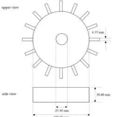
Figure 3 presents a schematic representation of the distributor dimensions. The distributor had a bottom opening (25.4 mm), through which the fluid entered axially until reaching the 16 radial outlets (6.35 mm) to leave the system.
Figure 3: Schematic representation and main geometric dimensions of the distributor used in the experimental apparatus
A digital Bourdon manometer, whose capacity was 5 bar (506625 Pa), was installed opposite to the axial inlet of liquid to measure the fluid pressure in the distributor (PD). Transparent, flexible, polyethylene pipes were connected to the 16 outlets to allow the fluid to return from the distributor to the tank. Each pipe was 3 m long and its diameter was 6.35 mm. The total length and diameter of the piping used between the tank and the distributor was 0.35 m and 25.4 mm, respectively.
Figure 4: Schematic representation of open (ON) and closed (OFF) distributor outlets in the tests in the experimental apparatus
Besides the aforementioned steps, the fluid volumetric flow rate (Qi) were measured in each open line using gravimetric techniques to verify the distributor efficiency to direct the volumetric flow rate captured (Q0) to the open outlets. To validate the hypothesis of constant pressure inside the distributor (PD), Computational Fluid Dynamics techniques (CFD) were applied to the flow inside the distributor, already presented in Figure 3. Table 1 shows the numerical conditions applied to the description of the flow inside the distributor [17, 18, 19].
Table 1. Numerical conditions applied to the description of the flow inside the distributor using Computational Fluid Dynamics techniques
Software FLUENT®
Turbulence Model Reynolds Stress Model (RSM)
Pressure-velocity coupling algorithm SIMPLEC
Interpolation scheme QUICK
Fluid and temperature (T) Water (293 K)
Number of computational cells (NC) 10000
Time Step (Δt) 0.0001 s
Number of exhausts simulated in CFD (N) 2, 8, and 16
Suction volumetric flow rate (Q0) 0.207, 0.739, and 1.118 L/s
Convergence criterion (δ) δ ≤ 0.0001
Discharge pressure (Pi) - Uberlândia (Brazil) 101325 Pa
Effect of the Main Factors on the Capacity of a Hydraulic System with Multiple Exhausts
The following factors can certainly affect the volumetric capacity of a hydraulic system with multiple exhausts: number of exhausts (N), length of discharge lines (L), diameter of discharge lines (D), relative roughness of discharge lines (ε/D), elevation of fluid exhaust (z), and pump power output (PPU). To evaluate the contribution of each variable to the volumetric capacity (Q0) of a hydraulic system with multiple exhausts, this section presents a Design of Experiments to determine these effects [20-21]. The relevant operational factors (N, L, D, ε/D, z, PPU) were organized in a Central Composite Design (CCD) according to the design matrix presented in Table 2 [22-23].
Table 2. Design matrix with α = 2.00
07 -1 [8] -1 [32.5] +1 [0.1016] +1 [0.0375] -1 [-5] -1 [2983] 08 -1 [8] -1 [32.5] +1 [0.1016] +1 [0.0375] +1 [+5] +1 [5965] 09 -1 [8] +1 [77.5] -1 [0.0508] -1 [0.0129] -1 [-5] +1 [5965] 10 -1 [8] +1 [77.5] -1 [0.0508] -1 [0.0129] +1 [+5] -1 [2983] 11 -1 [8] +1 [77.5] -1 [0.0508] +1 [0.0375] -1 [-5] -1 [2983] 12 -1 [8] +1 [77.5] -1 [0.0508] +1 [0.0375] +1 [+5] +1 [5965] 13 -1 [8] +1 [77.5] +1 [0.1016] -1 [0.0129] -1 [-5] -1 [2983] 14 -1 [8] +1 [77.5] +1 [0.1016] -1 [0.0129] +1 [+5] +1 [5965] 15 -1 [8] +1 [77.5] +1 [0.1016] +1 [0.0375] -1 [-5] +1 [5965] 16 -1 [8] +1 [77.5] +1 [0.1016] +1 [0.0375] +1 [+5] -1 [2983] 17 +1 [20] -1 [32.5] -1 [0.0508] -1 [0.0129] -1 [-5] +1 [5965] 18 +1 [20] -1 [32.5] -1 [0.0508] -1 [0.0129] +1 [+5] -1 [2983] 19 +1 [20] -1 [32.5] -1 [0.0508] +1 [0.0375] -1 [-5] -1 [2983] 20 +1 [20] -1 [32.5] -1 [0.0508] +1 [0.0375] +1 [+5] +1 [5965] 21 +1 [20] -1 [32.5] +1 [0.1016] -1 [0.0129] -1 [-5] -1 [2983] 22 +1 [20] -1 [32.5] +1 [0.1016] -1 [0.0129] +1 [+5] +1 [5965] 23 +1 [20] -1 [32.5] +1 [0.1016] +1 [0.0375] -1 [-5] +1 [5965] 24 +1 [20] -1 [32.5] +1 [0.1016] +1 [0.0375] +1 [+5] -1 [2983] 25 +1 [20] +1 [77.5] -1 [0.0508] -1 [0.0129] -1 [-5] -1 [2983] 26 +1 [20] +1 [77.5] -1 [0.0508] -1 [0.0129] +1 [+5] +1 [5965] 27 +1 [20] +1 [77.5] -1 [0.0508] +1 [0.0375] -1 [-5] +1 [5965] 28 +1 [20] +1 [77.5] -1 [0.0508] +1 [0.0375] +1 [+5] -1 [2983] 29 +1 [20] +1 [77.5] +1 [0.1016] -1 [0.0129] -1 [-5] +1 [5965] 30 +1 [20] +1 [77.5] +1 [0.1016] -1 [0.0129] +1 [+5] -1 [2983] 31 +1 [20] +1 [77.5] +1 [0.1016] +1 [0.0375] -1 [-5] -1 [2983] 32 +1 [20] +1 [77.5] +1 [0.1016] +1 [0.0375] +1 [+5] +1 [5965] 33 -α [2] 0 [55.0] 0 [0.0762] 0 [0.0250] 0 [0] 0 [4474] 34 + α [26] 0 [55.0] 0 [0.0762] 0 [0.0250] 0 [0] 0 [4474] 35 0 [14] -α [10.0] 0 [0.0762] 0 [0.0250] 0 [0] 0 [4474] 36 0 [14] +α [100.0] 0 [0.0762] 0 [0.0250] 0 [0] 0 [4474] 37 0 [14] 0 [55.0] -α [0.0254] 0 [0.0250] 0 [0] 0 [4474] 38 0 [14] 0 [55.0] +α [0.1270] 0 [0.0250] 0 [0] 0 [4474] 39 0 [14] 0 [55.0] 0 [0.0762] -α [0.0000] 0 [0] 0 [4474] 40 0 [14] 0 [55.0] 0 [0.0762] +α [0.0500] 0 [0] 0 [4474] 41 0 [14] 0 [55.0] 0 [0.0762] 0 [0.0250] -α [-10] 0 [4474] 42 0 [14] 0 [55.0] 0 [0.0762] 0 [0.0250] +α [+10] 0 [4474] 43 0 [14] 0 [55.0] 0 [0.0762] 0 [0.0250] 0 [0] -α [1492] 44 0 [14] 0 [55.0] 0 [0.0762] 0 [0.0250] 0 [0] +α [7456]
The factors mentioned previously were arranged in the following ranges: 2 ≤ N (-) ≤ 26; 10.0 ≤ L (m) ≤ 100.0; 0.0254 ≤ D (m) ≤ 0.1270; 0.0000 ≤ ε/D (-) ≤ 0.0500; -10 ≤ z (m) ≤ 10, and 1492 ≤ PPU (W) ≤ 7456. The factors N, L, D, ε/D,
z, and PPU were coded [Eq. (9)] and named as X1, X2, X3, X4, X5, and X6, respectively.
1
2
3
4
5
6
PU N 14
6 L 55.0
22.5 X
X D 0.0762
0.0254 X
X D 0.0250
0.0125 X
X z 0
5
P 4474
1492
(9)
factors (f0, f1, f2, ..., fi, ..., fN), and the absolute fluid pressure in the distributor (PD). Therefore, based on the fluid average velocities, the volumetric flow rates could be estimate in each exhaust (Qi) for each design matrix line (n). The addition of all these volumetric flow rates equaled the volumetric capacity (Q0).
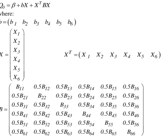
After estimating the volumetric capacity (Q0), multiple regression techniques were applied to obtain the Regression Equation [23]. It is generically represented by Eq. (10), which includes the average value (β), the linear effects (vector b), the quadratic effects (main diagonal of the matrix: Bii), and the cross-interaction effects (elements out of the main diagonal: Bij = Bji).
T 0
Q
bXX BX (10) where:
1 2 3 4 5 6
b b b b b b b
1
2
3
4
5
6 X X X X
X X X
T
1 2 3 4 5 6
X X X X X X X
11 12 13 14 15 16
21 22 23 24 25 26
31 32 33 34 35 36
41 42 43 44 45 46
51 52 53 54 55 56
61 62 63 64 65 66
B 0.5B 0.5B 0.5B 0.5B 0.5B
0.5B B 0.5B 0.5B 0.5B 0.5B
0.5B 0.5B B 0.5B 0.5B 0.5B
B
0.5B 0.5B 0.5B B 0.5B 0.5B
0.5B 0.5B 0.5B 0.5B B 0.5B
0.5B 0.5B 0.5B 0.5B 0.5B B
During the application of multiple regression techniques, only significant effects were considered, i.e., the ones that presented a significance level (p) lower or equal to 10%. Non-significant effects (p > 10%) were assigned value zero. The variation between the volumetric capacity and the factors analyzed here (∂Q0/∂X) was calculated by deriving Eq. (10) in the central point (line 45), according to Eq. (11). Next, the modules of the derivatives were estimated and compared, and then arranged them in ascending order to individually define the order of importance and the impact of each variable on the volumetric capacity of the system.
0 0 0 0 0 0 0
1 2 3 4 5 6
X 0 X 0 X 0 X 0 X 0 X 0 X 0
Q Q Q Q Q Q Q
X X X X X X X
(11)
Water at 20.0ºC ± 0.5ºC was the fluid used in the numerical implementation of the design matrix. Suction pressure (P0) and the exhaust pressures (P1, ..., Pi, .... PN) were considered at the atmospheric pressure in Uberlandia (Brazil) [24]. All exhausts had the same elevation according to the values defined in each design matrix line (n). The diameter (D0) and the length (L0) of pipe before the distributor remained the same in all simulations, namely 0.1207 m and 1.5 m, respectively.
RESULTS
Figure 5: Pressure profiles simulated by the CFD techniques with 2 (a), 8 (b), and 16 (c) exhausts
According to Figure 5, the geometric dimensions of the distributor were adequate and promoted a uniform distribution of pressure inside the device, which confirms the hypothesis initially presented in this study ( P 0).
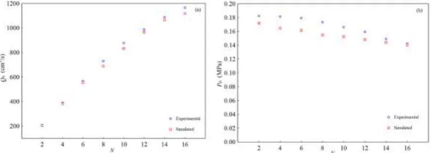
To validate physical-mathematical model proposed, the 2, 4, 6, 8, 10, 12, 14, and 16 discharge lines of the experimental apparatus were opened and experimentally measured the volumetric capacity (Q0) and the pressure (PD) in the distributor using a rotameter and a manometer, respectively. These operating conditions were also considered in the physical-mathematical model to theoretically predict these responses (Q0 and PD). Figure 6 displays the experimental and simulated results for Q0 and PD, respectively.
Figure 6: Comparison between the theoretical and experimental results for volumetric capacity (a) and absolute pressure inside the distributor (b) as a function of the number of exhausts (N)
Based on the comparison presented in Figure 6, the physical-mathematical model proposed in this study satisfactorily predicted the hydraulic system capacity and the pressure in the distributor considering the number of exhausts used. The average deviations between the theoretical prediction and the experimental measurements for Q0 and PD were 3% and 7%, respectively.
The results in Figure 6 also showed that the volumetric capacity increases directly with the number of exhausts. For example, the volumetric capacity of the experimental apparatus increased in about 5 times when the number of discharge lines changed from 2 to 16.
This is an interesting strategy to supply a higher demand for fluid from hydraulic systems that have already reached their maximum volumetric capacity and have only one pump installed in the circuit. The addition of exhausts simultaneously increased the perpendicular area available for flow (beneficial situation) and the pipe wall area (adverse situation) after the distributor. These two effects played opposite roles during the flow, but the beneficial situation certainly prevailed over the adverse situation, since the volumetric capacity of the hydraulic system presented an overall increase.
Figure 7 (a) illustrates the experimental volumetric flow rates of each discharge line (Qi) considering the hydraulic system working with 16 exhausts. Each individual volumetric flow rate was estimated in triplicate.
distributor was turbulent, and the fluid velocity presented instantaneous oscillations, which perfectly explains the results shown in Figure 7 (b). The CFD simulations have also shown that the individual volumetric flow rate (Qi) was stabilized in approximately 5 s. After this time, the individual volumetric flow rate had small fluctuations around the mean due to turbulence within the distributor.
Figure 7: Experimental distribution of individual flow rates (Qi) in all exhausts (a) and simulated individual flow rate in the specific exhaust (b)
In Figure 7 (a), the distributor did not equally divide the volumetric capacity to the many individual discharge lines, but it satisfactorily performed its work. The CFD simulations had already indicated that the flow inside the distributor was turbulent, and the fluid velocity presented instantaneous oscillations, which perfectly explains the results shown in Figure 7 (b). The CFD simulations have also shown that the individual volumetric flow rate (Qi) was stabilized in approximately 5 s. After this time, the individual volumetric flow rate had small fluctuations around the mean due to turbulence within the distributor.
At last, the proposed numerical method was satisfactorily to predict the volumetric capacity of a hydraulic system consisted of multiple exhausts. Thus, this methodology can be generalized and applied to other operating conditions to estimate the effects of the main variables on the system capacity, as demonstrated in the next section.
Quantification of the Effects of the Main Factors on the Volumetric Capacity of a Hydraulic System with Multiple Exhausts
Figure 8 presents the volumetric capacity (Q0) numerically obtained under the operating conditions for each line (n) of the design matrix (Table 2).
Figure 8: Fluid volumetric flow rates in the suction (a) and absolute pressure (b) in the distributor (simulated values) for each line (n) of the design matrix
Regression Equation was obtained to describe the phenomenon, as shown in Eq. (12). In this step, only the effects that presented a significance level (p) lower or equal to 10% were considered.
T T 1 1 2 2 3 3 0 4 4 5 5 6 6 X X
33.96 0 0 9.84 0 13.34 0
X X
18.57 0 0 5.02 0 6.66 0
X X
58.44 9.84 5.02 0 0 21.04 0
Q 108.74
X X
9.51 0 0 0 0 0 0
X X
48.52 13.34 6.66 21.
X X 9.69 1 2 3 4 5 6 X X X X X
04 0 0 0
X
0 0 0 0 0 0
(12)
According to the Regression Equation (R2 = 0.9844), all variables affected the capacity of the hydraulic system. All of
them presented significant linear effects. However, all quadratic effects were insignificant (B11= B22= B33= B44= B55=
B66= 0). The only relevant cross effects on Q0 were B13(N/D interaction), B23 (L/D interaction), B15 (N/z interaction),
B25 (L/z interaction), and B35 (D/z interaction).
To evaluate the isolated effect of each variable on the suction flow rate, the partial derivatives of the Regression Equation were estimated, whose results are presented in Eq. (13).
0 3 5 1 0 3 5 2 0
1 2 5
3
0
4
0
1 2 3
5
0
6 Q
33.96 19.69 X 26.69 X X
Q
18.57 10.04 X 13.32 X X
Q
58.44 19.69 X 10.04 X 42.09 X X
Q
9.51 X
Q
48.52 26.69 X 13.31X 42.09 X X Q 9.69 X (13)
The variations in the central point (X = 0) demonstrated that the number of discharge lines [X1/N], the diameter of the discharge lines [X3/D], and the pump power output [X6/PPU] positively affected the response analyzed (Q0). Among them, the piping diameter had the most significant impact (+58.44), followed by the number of exhausts (+33.96), and the pump power output (+9.69), in this order. On the other hand, some variations had negative effects on the capacity of the hydraulic system, such as the length of the discharge lines [X2/L], the relative roughness [X4/ε/D], and the elevation of exhausts [X5/z]. Among these negative effects, the level of exhausts had the most significant impact (-48.52), followed by the length of the discharge lines (-18.57), and the relative roughness (-9.51), in this order. For a generalized analysis of the six effects studied, Figure 9 shows the modules of the derivatives estimated in the central point (X = 0).
Based on Figure 9, the factors that most affected (major impacts) the capacity of the hydraulic system with multiple
exhausts were listed in ascending order, i.e.,
/ D
P
PU
L
N
z
D
. This list demonstrated that the piping diameter (D) had the highest impact on the volumetric capacity of a hydraulic system with multiple exhausts. It explains why the operating conditions of line n = 37 of the design matrix (Table 2) presented one of the lowest capacities among the ones obtained in the study (15.71 L/s).Certainly, the highest capacity of a hydraulic system like the one studied here could be obtained under the most favorable extreme conditions of the factors, i.e., +α, -α, +α, -α, -α, and +α for N, L, D, ε/D, z, and PPU, respectively. In this favorable operating condition, simulations indicated that the system could capture a volumetric flow rate of up to 5134 L/s.
Line 45 of Table 2 was chosen to analyze only the effect of the number of exhausts because the length (L), diameter (D), level of exhausts (z), relative roughness (ε/D), and pump power output (PPU) were remained constant. Then, discharge lines were added after the distributor (1 ≤ N ≤ 60). Figure 10 presents the volumetric capacity (Q0) and the individual flow rates of each exhaust (Qi). Additionally, the absolute pressure in the distributor (PD) in the multiple discharge lines (N) were followed.
Figure 10: Effect of the multiple exhausts (N) on the volumetric flow rate, individual flow rates (a), and pressure in the distributor (b) for the operating conditions of line n = 45
Therefore, although there are benefits, the addition of new discharge lines can have three limitations: one is physical and the other two are operational. The physical limitation says respect to the distributor size. As it is finite, the installation of too many discharge lines can not be possible in practice. The first operational limitation is the pressure level inside the distributor, which can stop the flow when it tends to the pressure of the discharge lines. The second operational limitation is the demand required in each piping line. The increase in the number of lines reduces the individual flow rate, which may not meet the user’s expectations. Therefore, if all the exhausts are made in the same reservoir, the final result will always be advantageous because the volumetric flow rate will be much higher than a traditional system (one exhaust only).
CONCLUSIONS
The addition of multiple exhausts had a significant influence on the volume capacity of a hydraulic system. From the Fluid Mechanics’s physical-mathematical point of view, this new system was more complex than the traditional one (single exhaust), because a set of nonlinear equations must be solved. For each discharge line added, there were two additional nonlinear equations to be solved. The numerical simulations were satisfactory; their deviations were lower than 4% when compared to the experimental measurements. The main results showed that the addition of multiple exhausts was beneficial for the hydraulic system, because it increased the volumetric flow rate with the same pump power installed. For example, the experimental measurements showed that changing the number of discharge lines from 2 to 16 increased the volumetric flow rate (suction) in 445%. The numerical method adopted, the CFD simulations, and the experimental measurements indicated that the most relevant factors on the performance of the hydraulic system were the piping diameter (D), the elevation of exhausts (z), and the number of exhausts (N), in this order. Their effects estimated in the central point were +58.44, -48.52, and +33.96, respectively. Finally, the methodology presented here was satisfactory. Any user can evaluate it to benefit from its resources so that the advantages of multiple discharge lines prevail over the eventual disadvantages.
NOMENCLATURE
b vector of linear effects (-)
B matrix of quadratic and cross effects (-) D diameter of discharge lines (m) f friction factor (-)
g gravitational acceleration (m/s2)
hC head loss (m)
hCL localized head loss (m)
hP pump head (m)
hT turbine head (m)
KS localized head loss coefficient (-)
L length of discharge lines (m) n number of design matrix lines (-) N number of exhausts (-)
NC number of computational cells (-)
p significance level
P absolute fluid pressure (Pa)
PD absolute fluid pressure in the distributor (Pa)
PP pump power (W)
PPU pump power output defined as PPηP (W)
Qi fluid volumetric flow rate in the exhaust "i" (L/s)
Q0 fluid volumetric flow rate (volumetric capacity) in the suction (L/s)
R2 variance
Re Reynolds number calculated at D (-) T fluid temperature (K)
v fluid flow average velocity (m/s) X coded variable
z elevation of exhaust (m) zi elevation of exhaust "i" (m)
zD elevation of the distributor (m) α orthogonality (-)
β independent term of the Regression Equation (L/s) δ convergence criterion (-)
∆t time step (s) ηP pump yield (-)
ρ fluid density (kg/m3)
σ1 upstream characteristic dimension (m)
σ2 downstream characteristic dimension (m)
ACKNOWLEDGEMENTS
The authors of this paper thank to the Brazilian research funding agencies FAPEMIG and CNPq and to the Separation Processes and Renewable Energy Laboratory (LASER) of the School of Chemical Engineering of the Federal University of Uberlandia (FEQUI/UFU) for the financial resources provided.
REFERENCES
[1] L.E. Sisson, D.R. Pitts, “Transport Phenomena”, Guanabara Dois, Rio de Janeiro, 1979.
[2] R.B. Bird, W.E. Stewart, E.N. Lightfoot, “Transport Phenomena”, second ed., John Wiley & Sons, New York, 2007.
[3] C.O. Bennet, J.E. Myers, “Transport Phenomena – Momentunm, Heat and Mass”, McGraw-Hill, New York, 1978.
[4] C.D. Argyropoulos, N.C. Markatos, “Recent advances on the numerical modelling of turbulent flows”, Appl. Math. Model. 39 (2015) 693–732, http://dx.doi.org/10.1016/j.apm.2014.07.001.
[5] W.H. Azmi, K.V. Sharma, P.K. Sarma, R. Mamat, S. Anuar, “Numerical validation of experimental heat transfer coefficient with SiO2 nanofluid flowing in a tube with twisted tape inserts”, Appl. Therm. Eng.73
(2014) 296-306, http://dx.doi.org/10.1016/j.applthermaleng.2014.07.060.
[6] H. Zambrano, L.D.G. Sigalotti, F. Pena-Polo, L. Trujillo, “Turbulent models of oil flow in a circular pipe with sudden enlargement”, Appl. Math. Model. 39 (2015) 6711–6724, http://dx.doi.org/10.1016/j.apm.2015.02.028.
[7] H. Tavassoli, E.A.J.F. Peters, J.A.M. Kuipe, “Direct numerical simulation of fluid–particle heat transfer in fixed random arrays of non-spherical particles”, Chem. Eng. Sci. 16 (2015) 42–48, http://dx.doi.org/10.1016/j.ces.2015.02.024.
[8] M. Magnini, B. Pulvirenti, J.R. Thome, “Characterization of the velocity fields generated by flow initialization in the CFD simulation of multiphase flows”, Appl. Math. Model. 40 (2016) 6811–6830, http://dx.doi.org/10.1016/j.apm.2016.02.023.
[9] S. Venkatachalapathy, G. Kumaresan, S. Suresh, “Performance analysis of cylindrical heat pipe using nanofluids - An experimental study”, Int. J. Multiphase Flow 72 (2015) 188-197, http://dx.doi.org/10.1016/j.ijmultiphaseflow.2015.02.006.
[10]S. Schneiderbauer, S. Pirker, “Determination of open boundary conditions for computational fluid dynamics (CFD) from interior observations”, Appl. Math. Model. 35 (2011) 763–780, http://dx.doi.org/10.1016/j.apm.2010.07.032.
[11]C. Liu, J. Wolfersdorf, Y. Zhai, “Comparison of time-resolved heat transfer characteristics between laminar and turbulent with unsteady flow temperature”, Int. J. Heat Mass Transfer 84 (2015) 376-389, http://dx.doi.org/10.1016/j.ijheatmasstransfer.2015.01.034.
[12]Z. Guo, D.F. Fletcher, B.S. Haynes, “Implementation of a height function method to alleviate spurious currents in CFD modelling of annular flow in microchannels”, Appl. Math. Model. 39 (2015) 4665– 4686, http://dx.doi.org/10.1016/j.apm.2015.04.022.
[13]A.S. Foust, C.W. Clump, Princípios das Operações Unitárias, LTC, São Paulo, 1982.
[14]J. Pérez-García, E. Sanmiguel-Rojas, A. Viedma, “New experimental correlations to characterize compressible flow losses at 90-degree T-junctions”, Exp. Therm. Fluid Sci. 33 (2009) 261-266, http://dx.doi.org/10.1016/j.expthermflusci.2008.09.002.
[15]J. Pérez-García, E. Sanmiguel-Rojas, J. Hernández-Grau, A. Viedma, “Numerical and experimental investigations on internal compressible flow at T-type junctions”, Exp. Therm. Fluid Sci. 31 (2006) 61-74, http://dx.doi.org/10.1016/j.expthermflusci.2006.02.001.
[16]L.A. Andrade, M.S.A. Barrozo, L.G.M. Vieira, “A study on dynamic heating in solar dish concentrators”, Renew. Energy 87 (2016) 501-508, http://dx.doi.org/10.1016/j.renene.2015.10.055.
[17]L.G.M. Vieira, M.A.S. Barrozo, “Effect of vortex finder diameter on the performance of a novel hydrocyclone separator”. Miner. Eng. 57 (2014) 50-56, http://dx.doi.org/10.1016/j.mineng.2013.11.014. [18]L.G.M. Vieira, D.O. Silva, M.A.S. Barrozo, “Effect of inlet diameter on the performance of a filtering
hydrocyclone separator”. Chem. Eng. Technol. 39 (2016) 1406-1412, http://dx.doi.org/10.1002/ceat.201500724.
[19]E.V. Kartaev, V.A. Emelkin, M.G. Ktalkerman, S.M. Aulchenko, S.P. Vashenko, V.I. Kuzmin, “Formation of counter flow jet resulting from impingement of multiple jets radially injected in a
crossflow”, Exp. Therm. Fluid Sci. 68 (2015) 310-321,
[20]F.F. Salvador, M.A.S Barrozo, L.G.M. Vieira, “Effect of a cylindrical permeable wall on the performance of hydrocyclones”, Chem. Eng. Technol. 39 (2016) 1015-1022, http://dx.doi.org/10.1002/ceat.201500246.
[21]N.K.G. Silva, D.O. Silva, L.G.M. Vieira, M.A.S. Barrozo, “Effects of underflow and vortex finder length on the performance of a newly designed filtering hydrocyclone”, Powder Technol. 286 (2015) 305-310, http://dx.doi.org/10.1016/j.powtec.2015.08.036.
[22]M.J. Box, W.G. Hunter, J.S. Hunter, “Statistics for Experiments: an introduction to design, data analysis and model building”, John Wiley and Sons, 1978.
[23]R.H. Myers, “Response Surface Methodology”, Edwards Brother, 1976.
![Table 2. Design matrix with α = 2.00 X [D (m)] X [ε/D (-)] X](https://thumb-us.123doks.com/thumbv2/123dok_us/8683729.1734112/5.595.77.547.72.305/table-design-matrix-a-x-d-x-e.webp)