Spatial patterns in bacterial community structure and function within shallow alpine tarns

(1)

Lincoln

University

Digital

Thesis

Copyright

Statement

The

digital

copy

of

this

thesis

is

protected

by

the

Copyright

Act

1994

(New

Zealand).

This

thesis

may

be

consulted

by

you,

provided

you

comply

with

the

provisions

of

the

Act

and

the

following

conditions

of

use:



you

will

use

the

copy

only

for

the

purposes

of

research

or

private

study



_you

_will

_recognise

_the

_author's

_right

_to

_be

_identified

_as

_the

_author

_of

_the

_thesis

_and

due

acknowledgement

will

be

made

to

the

author

where

appropriate



_you

_will

_obtain

_the

_author's

_permission

_before

_publishing

_any

_material

_from

_the

thesis.

(2)

Spatial Patterns in Bacterial Community

Structure and Function within Shallow Alpine

Tarns

A thesis

submitted in partial fulfilment

of the requirements for the Degree of

Master of Science

at

Lincoln University

by

Julia Ruth Bellamy

(3)

Spatial Patterns in Bacterial Community Structure and Function

within Shallow Alpine Tarns

by

Julia Ruth Bellamy

Small scale spatial variation in bacterial community structure and function in freshwater

ecosystems is poorly understood. I investigated the spatial variation of bacterial

communities within three tarns located at Tekapo Scientific Reserve using automated

ribosomal intergenic spacer analysis (ARISA). I examined the variability in bacterial

community structure both within and among tarn locations and explored whether bacterial

communities adhere to the same biogeographical patterns commonly reported for

communities of larger organisms; these were the taxa-area and distance-decay relationships.

I also attempted to identify physicochemical variables that were significantly related to the

observed community heterogeneity. To achieve these aims, I collected more than 100

samples in total across the three tarns and measured a range of physicochemical variables

(pH, conductivity, total carbon and anion concentrations) for each sample. The ARISA data

revealed significant variability in bacterial community structure among the tarns and some

variation within the tarns that was related to correlated spatial variability in a range of

physicochemical variables such as, pH, total carbon and conductivity. Distance-decay and

taxa-area relationships in bacterial community similarity were also observed. There was no

correlation between the structural and functional attributes (i.e., carbon substrate utilisation

patterns) of the bacterial communities, suggesting that there was some functional

redundancy in these bacterial communities in terms of carbon substrate utilisation. This

study provides valuable information about how freshwater bacterial biodiversity is

maintained and expands our understanding of the link between bacterial community

structure and function.

Keywords: Biogeographical patterns, taxa-area, z-value, distance-decay, ARISA, BIOLOG

(4)

Acknowledgements

First and foremost, I would like to thank Dr. Gavin Lear at the University of Auckland, NZ, for

his patience and guidance throughout the duration of this study. I would also like to thank

Dr. Hannah Buckley at Lincoln University, NZ, for her significant contribution towards this

study, especially in regards to data analysis and interpretation. I am grateful to Bradley Case,

also at Lincoln University, NZ, for his help with the GIS program, ArcMap 10. Finally, the kind

assistance with sample collection by Jack Lee and Taiga Yamamura was much appreciated.

(5)

List of Tables

Table 1. Samples required for analyses and storage conditions. ... 17 Table 2. Reagents used to create a mastermix suitable for the PCR amplification of DNA

for ARISA for one sample. ... 20 Table 3. Conditions under which the PCR was performed. ... 21 Table 4. Average water chemistry obtained for samples abstracted from each tarn. Data

are means ± standard error. ... 36 Table 5. Relationship of different environmental variables with bacterial community

structure. Environmental variables in bold were identified as being significant (P < 0.05). Subscript numbers indicate the order of significance of the

environmental variables (forward selection) and the % represents the proportion that each environmental variable contributed towards total

variation. Depth was only measured for samples in Tarn 3. ... 44 Table 6. Relationship of different environmental variables with bacterial community

function. Environmental variables in bold were identified as being significant (P < 0.05). Subscript numbers indicate the order of significance of the

environmental variables (forward selection) and the % represents the proportion that each environmental variable contributed towards total

variation. Depth was only measured for samples in Tarn 3. ... 44

Table A. 1. Carbon sources in BIOLOG EcoPlate™ (BIOLOG Inc, Hayward, CA, U.S.A.). Each plate contains triplicate replicates of the carbon sources. ... 60 Table A. 2. Sample of tabulated ARISA data. Columns are samples and the data in each

(8)

List of Figures

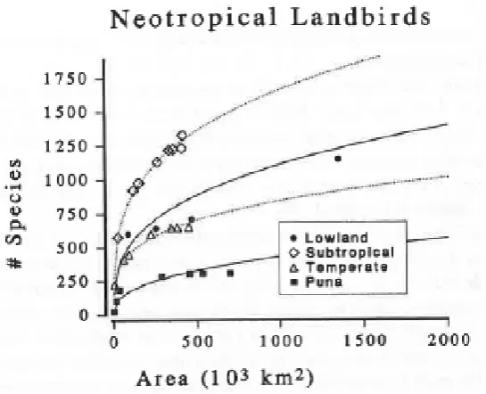
Figure 1. Taxa-area relationship modelled by the power law and plotted in arithmetic space showing an increase in species richness with increasing area. Taken

directly from Rosenzweig (1995). ... 2 Figure 2. Relationship between the compositional similarity of paired Inga communities

and geographic distance. Taken directly from Dexter et al. (2012). ... 4 Figure 3. Lake Mendote and Crystal Bog. Principle coordinate analysis (PCoA) was

performed on the bacterial community composition in the lakes and the axis of the ordinations were coloured and this information was plotted on the maps. Similar colours denote sites represented by more similar bacterial

communities. Taken directly from Jones et al. (2012). ... 7 Figure 4. Schematic of possible relationships between functional and species diversity. A1,

every species has a unique functional role resulting in a ratio of 1:1 between functional and species diversity; A2, multiple species have similar functional attributes; B, at low species richness, functional diversity rapidly increases and then increases at declining rates with high species diversity, and eventually reaches an asymptote; C, relationship between functional diversity and species diversity is sensitive to changes in environmental variables. Taken

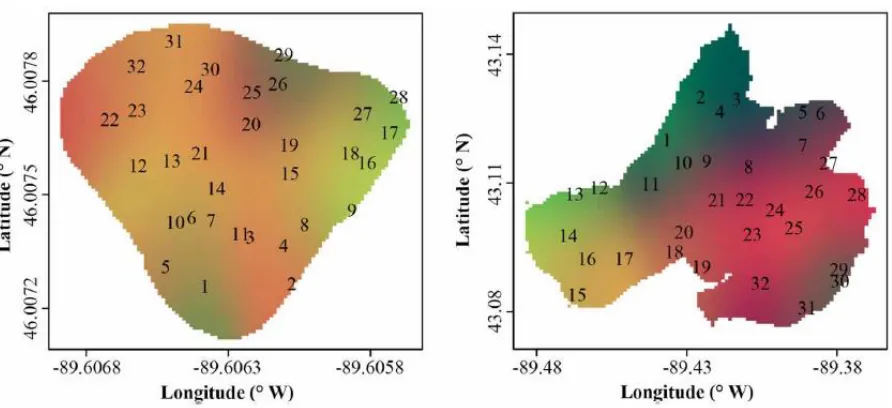
directly from Guillemot et al. (2011). ... 8 Figure 5. Location of tarns near Lake Tekapo, New Zealand. ... 14 Figure 6. Sample locations in the three tarns from which samples were collected. Each dot

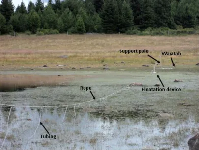
shows where water samples, and other data were collected. ... 14 Figure 7. Schematic showing the components of the sampling apparatus. The adjustable

support poles extended to a height of 2.5 m and the rope was 100 m long

giving us the ability to sample across a distance of 50 m (not to scale). ... 15 Figure 8. One of the support poles with attached rope and tubing of the sampling

apparatus. ... 16 Figure 9. Floatation device that was used to collect water from a depth of 5 cm. ... 16 Figure 10. Buchner filter showing a Buchner funnel (Nalgene®, Thermo SCIENTIFIC,

Rochester, NY, U.S.A.) and the waste collection container (KIMAX®, KIMBLE, Vineland, NJ, U.S.A.). ... 18 Figure 11. Unused BIOLOG EcoPlate™ (left) and BIOLOG EcoPlate™ (right) showing colour

development. ... 23 Figure 12. Example of variance partitioning displayed on a column plot. Four different

components are shown: (hatched) unexplained variation; (black) pure environmental variation that is independent of any spatial factors; (white) pure spatial variation that is independent of any environmental variables;

(grey) spatially structured environmental variables. ... 28 Figure 13. Taxa-area relationship for each tarn. The cumulative number of samples (mean

taxa richness was calculated for each combination of samples) was used to represent area. The relationship in each tarn was modelled by the power law

(S = cAz, red line = fitted values). ... 30

(9)

Figure 15. Differences in bacterial community structure (left) and bacterial community function (right). Plots are non-metric multidimensional scaling of ARISA data and carbon substrate utilisation data, using Bray-Curtis similarity matrices of samples. Data points relate to samples abstracted from Tarn 1, 2 or 3. Two-dimensional stress values are 0.20 and 0.18 for plots of bacterial community structure and function, respectively. ... 33 Figure 16. Similarity in bacterial community structure and function among tarns. Bacterial

community data for each tarn were subjected to a data reduction procedure by non-metric multidimensional scaling of Bray-Curtis similarity data. The differences between the highest and lowest 1-d configuration scores for each plot were then used to classify the configuration into ten equally sized classes. The bacterial community data falling within each class was assigned a

different colour, across a gradient from dark blue (lowest 1-d configuration score) to light green (highest 1-d configuration score. The outcome of this approach is that samples hosting more similar bacterial community data are represented by more similar colours on each map... 35 Figure 17. Example of a dendrogram for bacterial community structure in Tarn 1 showing

the cut off at 50 % (red line) Bray-Curtis similarity. Each branch that the red line crosses is a different cluster in the tarn at the 50 % Bray-Curtis similarity level. ... 37 Figure 18. Variation in bacterial community structure in each tarn. Plots are derived from

non-metric multidimensional scaling of ARISA data using a Bray-Curtis similarity measure. Group average clusters are superimposed on each plot (red circles) at the level of 50 % Bray-Curtis similarity. Each sample that is not constrained was in its own cluster. Two-dimensional stress values are 0.16, 0.13 and 0.13, respectively. ... 38 Figure 19. The plots on the left show similarity in bacterial community structure within

the tarns. Bacterial community data for each tarn were subjected to a data reduction procedure by non-metric multidimensional scaling of Bray-Curtis similarity data. The differences between the highest and lowest 1-d

configuration scores for each plot were then used to classify the configuration into ten equally sized classes. The bacterial community data falling within each class was assigned a different colour, across a gradient from dark blue (lowest 1-d configuration score) to light green (highest 1-d configuration score). The outcome of this approach is that samples hosting more similar bacterial community data are represented by more similar colours on each map. The plots on the right show the physical location of the different clusters within the tarns. Each colour represents a different cluster with black

representing individual samples that did not fall within the main clusters. ... 40 Figure 20. Similarity in bacterial community structure and function within the tarns.

Bacterial community data for each tarn were subjected to a data reduction procedure by non-metric multidimensional scaling of Bray-Curtis similarity data. The differences between the highest and lowest 1-d configuration scores for each plot were then used to classify the configuration into ten equally sized classes. The bacterial community data falling within each class was assigned a different colour, across a gradient from dark blue (lowest 1-d configuration score) to light green (highest 1-d configuration score. The outcome of this approach is that samples hosting more similar bacterial

(10)

Figure 21. Contour plots of significant environmental variables. A = nitrite-N, Tarn 1; B = total carbon, Tarn 2; C = sulphate-S, Tarn 2; D = pH, Tarn 3; E = total carbon, Tarn 3; F = depth, Tarn 3. The difference between the highest and lowest value for each environmental variable was used to classify the data for each variable into ten equally sized classes. The environmental data falling within each class was assigned a different colour, across a gradient from dark blue (lowest 1-d configuration score) to light green (highest 1-d configuration score). The outcome of this approach is that samples hosting more similar environmental values (for the selected environmental variable) are

represented by more similar colours on each map... 45 Figure 22. Results of partial regression analysis, partitioning the variation in bacterial

community structure within each of the three tarns (data for each tarn analysed individually), or among all tarns (data for all three tarns analysed together). Four different components are shown: (hatched) unexplained variation; (black) pure environmental variation that is independent of any spatial factors; (white) pure spatial variation that is independent of any

environmental variables; (grey) spatially structured environmental variables. ... 47 Figure 23. Results of partial regression analysis, partitioning the variation in bacterial

community function within each of the three tarns (data for each tarn analysed individually), or among all tarns (data for all three tarns analysed together). Four different components are shown: (hatched) unexplained variation; (black) pure environmental variation that is independent of any spatial factors; (white) pure spatial variation that is independent of any

environmental variables; (grey) spatially structured environmental variables. ... 47

Figure A. 1. Variation in bacterial community function in each tarn. Plots are derived from non-metric multidimensional scaling of ARISA trace data using a Bray-Curtis similarity measure. Group average clusters are superimposed on each plot at the level of 50 % Bray-Curtis similarity. Two-dimensional stress values are

0.18, 0.14 and 0.19, for tarns 1, 2, and 3, respectively. ... 65 Figure A. 2. Diagram of how the variation attributable to different components is

calculated. Taken directly from Clarke and Gorley (2006) ... 66 Figure A. 3. DistLM output in PRIMER-E showing the proportion of variation calculated for

the different components. The numbers in the coloured bubbles are the

(11)

Chapter 1 Introduction

An important focus of ecology is to understand how biodiversity is generated and

maintained. This can, in part, be achieved through understanding the spatial distribution of

organisms (Green and Bohannan, 2006). However, while the distribution of larger organisms

is well documented (Rosenzweig, 1995), the biogeography of other groups of organisms,

such as, microorganisms remains poorly understood (Fierer and Jackson, 2006; Green and

Bohannan, 2006; Martiny et al., 2006). This is partly due to the fact that until recently we

relied on culture based techniques to identify microorganisms. It is proposed that less than

0.5 % of microorganisms can be cultured (Torsvik et al., 1990),such that a large proportion

of the microbial community is not detectable using such methods. However, with the

introduction of molecular techniques, microorganisms can now be rapidly characterised by

their DNA, removing the need to grow cells in the laboratory (Malik et al., 2008). Molecular

based techniques also allow microorganisms to be detected in situ (Gilbride et al., 2006).

Consequently, interest in microbial ecology continues to increase.

There is controversy surrounding the distribution of microorganisms. Some argue that all

microbial taxa are everywhere (cosmopolitan distribution) (Martiny et al., 2006), since the

small size and high abundance of microorganisms means that they are widely distributed in

large numbers in global currents of wind and water. Conversely, others claim that

microorganisms display biogeographical patterns, such as the species-area and

distance-decay relationships (Green and Bohannan, 2006; Horner-Devine et al., 2004; Martiny et al.,

2006), which suggests that there are barriers or limitations to microbial immigration or

(12)

1.1 Taxa-area relationship

A common biogeographical pattern reported for communities of macroorganisms is the

species, or taxa-area relationship (Crawley and Harral, 2001; Fridley et al., 2005; Rosenzweig,

1995; Ulrich and Buszko, 2003). The taxa-area relationship states that taxa richness increases

in accordance with area sampled (Lomolino, 2001). There are a number of formulae used to

model the taxa-area relationship (Scheiner, 2003), with the power law, Arrehenius (1921),

being one of the most commonly used:

S = cA

z

where S is species or taxa richness (number of species), A is area sampled, c is a constant

that partially determines the slope of the curve with z which is a measure of the rate of taxa

turnover across space. A larger z value represents a greater rate of turnover (Rosenzweig,

1995; Zhou et al., 2008). For example, the taxa-area relationship was modelled using the

power law in arithmetic space for South American birds in four biomes types and shows the

expected increase in species richness with increasing area sampled (Rosenzweig, 1995)

(Figure 1).

(13)

With the taxa-area relationship, it is important to understand that there is a difference in the

z-values for islands and contiguous habitats, which may be because islands are surrounded

by a barrier that hinders colonisation, whereas contiguous habitats can be colonised from

adjacent areas (Bell et al., 2005). With islands, z-values typically range from 0.25 to 0.35

(Rosenzweig, 1995). However, with contiguous habitats, z-values usually range from 0.12 to

0.18 (Rosenzweig, 1995). These z-values are for macroorganisms, so it is possible that they

may be different for microorganisms. It has been proposed that because the small size and

high abundance of microorganisms means that they are widely distributed, this will result in

lower z-values for microorganisms than for macroorganisms (Bellet al., 2005). Cencini et al.

(2012) determined that as the size of the local population increases, the species-area curve

become shallower (lower z-value), which is consistent with the theory that because

microorganisms are widely distributed, they will have a higher local population and hence

lower z-values than macroorganisms. Alternatively, microorganisms may have lower z-values

than macroorganisms due to decreased local diversification, because large population sizes

result in low extinction rates (Fenchel and Finlay, 2004), or low speciation rates due to

horizontal gene transfer (Thomas and Nielsen, 2005) and lack of geographical isolation

(Finlay, 2002).

The taxa-area relationship can be explained by three possible theories. First, it is likely that

more taxa will be encountered when sampling a larger area than a smaller area because

there is a higher probability that rare taxa will be encountered (Hill et al., 1994; Kallimanis et

al., 2008). Second, a larger area will be more environmentally heterogeneous and will thus

support a greater variety of taxa, each of which may be specialised to different

environmental conditions (Cam et al., 2002; Kallimanis et al., 2008; Preston, 1962;

Rosenzweig, 1995). Finally, the island biogeography theory which states that a dynamic

equilibrium exists between immigration and extinction rates on an island (MacArthur and

Wilson, 1967), and can be used to qualitatively predict shifts in species richness and turnover

rates with changes in area sampled and degree of isolation. One of the first studies to

identify a taxa-area relationship for microbial communities was performed by Bell et al.

(2005). Bell et al. (2005) observed a taxa-area relationship for microbial communities in

water-filled tree holes (islands). This study was performed over a relatively small spatial

scale with the largest island sampled (volume of water) being 20 litres. In contrast to Bell et

(14)

communities from six reservoirs of different sizes (maximum volumes ranged from 0.6 to

1700 Mm3) in Burkina Faso or three alpine lakes (maximum volumes ranged from 1124 to

8900 Mm3) in France. The inconsistency in these findings may be due to differences in the

scale of the studies as Bell et al. (2005) concluded that with large areas of contiguous habitat

the slope of the taxa-area relationship appears reduced. Alternatively, microbial

communities in freshwater ecosystems may not display taxa-area relationships because

freshwater systems are usually well mixed and environmental heterogeneity is low (Scheiner

et al., 2000). These studies highlight the importance of understanding the distribution of

microorganisms at various spatial scales.

1.2 Distance-decay relationship

Another common biogeographical pattern described in literature is the distance-decay

relationship (Dexter et al., 2012; Finkel et al., 2012; Jones et al., 2012; King et al., 2010;

Palmer, 2005; Sommaruga and Casamayor, 2009; Thieltges et al., 2009). The distance-decay

relationship states that community similarity declines with increasing geographic distance

(Horner-Devine et al., 2004). For example, this relationship was observed by Dexter et al.

(2012), who identified that the compositional similarity of Inga (a genus of nitrogen fixing

tree) communities in Madre de Dios, Peru for terra firme and floodplain showed a decline

with increasing geographic distance (Figure 2).

(15)

Two mechanisms may be responsible for the distance-decay relationship. First, because

microorganisms may have limited dispersal ability, community similarity will show a decline

with increasing geographic distance regardless of environmental features (Soininen et al.,

2007). Second, increasing environmental heterogeneity with increasing geographic distance

will result in a decline in community similarity with increasing distance. This is because

microorganisms are adapted to different environmental conditions which change over space

and will therefore be present where favourable conditions exist. For example, the landscape

structure and the degree of isolation of the landscape may influence the dispersal rate of

microorganisms (Nekola and White, 2004). The similarity of communities within a complex

landscape structure that has dispersal barriers will decline more abruptly than a less

complex and more open landscape. Also, landscapes that are more isolated will take longer

to colonise resulting in a gradient in microbial diversity after a disturbance.

Horner-Devine et al. (2004) analysed whether or not microorganisms displayed a taxa-area

relationship, using a distance-decay approach, in a New England salt marsh, and determined

that environmental heterogeneity affects microbial communities more than geographic

distance. It was found that when the effect of geographic distance was removed, habitats

with similar environmental conditions had similar microbial communities. However, when

the effect of environmental similarity was removed, geographic distance had no effect on

the microbial communities. This was supported by Van der Gucht et al. (2007), who

concluded that spatial distance is insignificant compared to local environmental conditions.

Finkel et al. (2012) investigated the dispersal limitation in phyllosphere communities on the

leaf surfaces of spatially dispersed, salt-excreting Tamarix trees. The trees were located over

a 500 km east-west transect in the Sonoran Desert of southwestern United States with

relatively uniform climate conditions (minimising environmental heterogeneity). They found

that some communities of bacterial taxa, such as betaproteobacteria, showed a significant

decline in similarity with increasing geographic distance. However, even though the sampling

regime was designed to minimise environmental heterogeneity, a weak relationship was

observed between geographic distance and environmental heterogeneity. This study

indicates that the distance-decay relationship can be observed for microorganisms over a

relatively large spatial scale (0 to 500 km). However, will it still be present over finer spatial

(16)

In regards to the distance-decay relationship being present over a range of spatial scales,

King et al. (2010), determined that the dissimilarity in bacterial community composition in

soil samples collected from a continuous landscape on the south side of the Green Lakes

Valley Watershed, Colorado, USA, only showed an increase between 2 to 240 m. However, in

contrast to Finkel et al. (2012), between 240 to 2000 m King et al. (2010) observed no

relationship between dissimilarity in bacterial community composition and geographic

distance. Spatial differences in bacterial community composition for samples that were

located less than 240 m apart were suggested to be due to the landscape distribution of

biogeochemical properties (King et al., 2010). These studies indicate that environmental

heterogeneity is a significant driver of the distance-decay relationship for microorganisms,

but also suggest that spatial location has some influence on the distance-decay relationship.

In addition, it has been identified that the distance-decay relationship might not be present

at all spatial scales.

1.3 Relationship between spatial scaling and efficient sampling strategies

The spatial scale of variation in microbial diversity may result in microbial communities that

are separated on a small scale of less than a metre being significantly different from each

other in terms of their composition (Franklin and Mills, 2003). The difference in microbial

communities may be due to variation in local, or microsite, conditions such as pH, organic

matter content or interactions with biological neighbours. Unfortunately, many sampling

regimes do not take this into consideration and in analysing only a limited number of

samples, they underestimate total microbial diversity (Mocali and Benedetti, 2010). The

spatial structure of microbes is poorly understood because a large number of samples are

typically required to accurately determine spatial variation (Saetre and Bååth, 2000).

However, recent advances in the high throughput analysis of microbial DNA now allow the

simultaneous analysis of hundreds of samples at a relatively low cost. A previously

mentioned study, Humbert et al. (2009), involved samples being collected from only one

location in reservoirs in individual lakes in Burkina Faso and alpine lakes in France because it

was concluded in an earlier study (Dorigo et al., 2006) that one sample provides a good

evaluation of the total bacterial diversity in a freshwater ecosystem. However, this is not

(17)

analyse the variation in bacterial community composition on a small spatial scale (10 m).

They identified significant horizontal variation in bacterial community composition across

the lakes (Figure 3). These studies suggest that even though microbial diversity may appear

to be relatively homogeneous across freshwater ecosystems nevertheless it may display

small scale spatial patterns. Therefore it is important to collect multiple samples across

freshwater ecosystems in order to provide an accurate representation of the microbial

community present.

Figure 3. Lake Mendote and Crystal Bog. Principle coordinate analysis (PCoA) was performed on the bacterial community composition in the lakes and the axis of the ordinations were coloured and this information was plotted on the maps. Similar colours denote sites represented by more similar bacterial communities. Taken directly from Jones

et al. (2012).

1.4 Link between microbial community structure and function

Microorganisms have a significant influence on important ecological processes in the

environment, such as trace gas emissions, soil structure and formation, decomposition of

organic matter and xenobiotics, and the recycling of essential elements (e.g. carbon,

nitrogen, phosphorous, and sulphur) and nutrients (Green and Bohannan, 2006;

Horner-Devine et al., 2004; Rastogi and Sani, 2011). The fact that microorganisms are involved in a

number of important ecological processes, along with the recent development of molecular

(18)

Tiedje, 2000; Horner-Devine et al., 2004; Reche et al., 2005; Van Der Gast et al., 2005) being

performed on microorganisms in relation to their distribution, which contributes to our

understanding of biodiversity. However, there remains limited information regarding the link

between the variation in microbial composition and the functional attributes of the

communities in natural ecosystems. It has been proposed that the number of species

required to sustain ecosystem functioning is directly correlated with the number of

processes considered (Hector and Bagchi, 2007) and there are a number of different

scenarios that can be used to model the relationship between functional diversity and

species diversity (Figure 4). A number of studies have attempted to identify the link between

microbial composition and ecological processes.

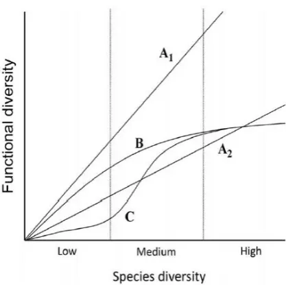
Figure 4. Schematic of possible relationships between functional and species diversity. A1, every species has a unique functional role resulting in a ratio of 1:1 between functional and species diversity; A2, multiple species have similar functional attributes; B, at low species richness, functional diversity rapidly increases and then increases at declining rates with high species diversity, and eventually reaches an asymptote; C, relationship between functional diversity and species diversity is sensitive to changes in environmental variables. Taken directly from Guillemot et al. (2011).

Balser and Firestone (2005) performed a study investigating the link between microbial

community composition and soil process rates such as N mineralisation, nitrification, CO2

and N2O flux, independent of certain environmental variables (soil temperature and water

(19)

conifer forest ecosystem, along an elevation gradient with different climates (temperature

and precipitation). Not only did they find that there was a significant relationship between

microbial community composition and soil processes independent of soil temperature and

water content, but soil processes were also related to the environment. Unfortunately, this

study only controlled soil temperature and water content and it is possible that there were a

number of other environmental variables that would have affected the soil processes.

Another study by Eilers et al. (2010) analysed shifts in bacterial community phylogenetic

structure in soils following the addition of specific carbon compounds (glucose, glycine and

citric acid). They found that the magnitude of the change in function (CO2 respiration) in

bacterial communities upon the addition of carbon compounds did not correlate with the

change in bacterial community composition. An increase in the abundance of a subset of

taxa was observed when the carbon compounds were added to the soil. However, a number

of abundant taxa showed no response to the addition of the carbon compounds. This study

shows that there is a link between bacterial community composition and ecological

processes to some degree but also indicates that microbial communities may exhibit some

functional redundancy. Functional redundancy is defined by Wohl et al. (2004) as “multiple

species, while biologically unique, contributing with similar intensity to the same process

within an ecosystem, such as energy flow or nutrient cycling”. It is evident from the study by

Balser and Firestone (2005) that there is variation in the functional attributes of microbial

communities in soil ecosystems. Is this relationship also present in freshwater ecosystems,

which can be expected to be less heterogeneous, due to mixing (Scheiner et al., 2000), or

will the microbial communities in these ecosystems show functional redundancy?

It is possible that microbial communities contain some functional redundancy. The high

species richness that is usually displayed by microorganisms is thought to facilitate

functional redundancy because the probability of encountering multiple species that

perform the same ecological processes is increased. An important question in microbial

ecology is, if a microbial community suffers from a disturbance that results in a loss of

biodiversity, will the new community be functionally similar to the original community or will

a loss in ecological processes be observed? Functional redundancy can be observed in two

different ways: (i) First, the new community may be compositionally different (e.g. contain

different taxa). However, it may still be capable of performing the same ecological processes

(20)

the community but individual taxa may function differently resulting in the same process

rate at the community level (Allison and Martiny, 2008). Alternatively, microbial

communities may display functional dissimilarity where a loss in the number of microbial

taxa corresponds to a loss in ecological processes. Microbial communities showing both

functional redundancy and functional dissimilarity have been observed in a range of studies.

Yin et al. (2000) performed a study that involved a number of soil samples from a soil

reclamation gradient in a tin mine site in Brazil being amended with different carbon

compounds (L-serine, L-threonine, sodium citrate, and α-lactose hydrate). A change in the

functional attributes of the bacterial communities would be expected upon the addition of

the carbon substrates and the corresponding amount of change or no change in the richness

and diversity of the bacterial communities would give an indication of the degree of

functional redundancy present in the bacterial communities. The richness and diversity of

bacterial groups increased along the reclamation gradient in response to the addition of the

carbon substrates, indicating some functional dissimilarity in the bacterial communities

because the modification in environment conditions supported the growth of new bacterial

taxa. However, even though some functional dissimilarity was observed, it was determined

that bacterial functional redundancy was positively correlated with changes in soil that

supported plant growth. Wohl et al. (2004) investigated functional redundancy by analysing,

under constant environmental conditions, if an increase in species richness influenced

function (cellulose decomposition) and if a decline in species richness was observed over

time in functionally redundant communities. It was observed that, in contrast to what was

expected, a decline in species richness only occurred for microcosms inoculated with two

species (one species was eliminated). Species richness was maintained in the other

microcosms that were inoculated with four or more species which was thought to be due to

the inherent diversity of multiple species that allowed for different resources to be

exploited. This implies that a functionally redundant community can support high species

richness through the production of resources by individuals resulting in resource

heterogeneity. The study also found that species richness was the main driver of function

(cellulose decomposition) with the microcosms that contained four or eight species

displaying the highest cellulose decomposition. Finally, Strickland et al. (2009) performed a

study that involved sterilised litter being inoculated with soil, both of which were collected

(21)

litter decomposition (measured by carbon mineralisation) was explained by the inoculum

source. This supports the idea of functional dissimilarity, that is, species perform unique

functions. These studies are evidence of research being performed to look at the functional

attributes of microbial communities in which the link between microbial composition and

function remains poorly understood (Guillemot et al., 2011), especially in freshwater

ecosystems. Unfortunately, the majority of the aforementioned studies were temporal

based and it would have been interesting if the studies had incorporated spatial parameters

into the investigation of functional diversity. In addition, previous studies investigated the

functional attributes of microbial communities by amending their habitat and then

monitoring the response of the microbial communities to this change instead of determining

functional redundancy in an undisturbed environment.

1.5 Aims, objectives and hypotheses

My study characterises spatial variability in bacterial community structure and functional

characteristics within tarns (shallow mountain lakes) located at Tekapo Scientific Reserve.

The influences of geographical distance and sample area on the bacterial communities were

investigated to examine concepts related to patterns of distance-decay and taxa-area

relationships, respectively. More than 100 bacterial community samples were collected

using a custom built sampling apparatus that minimised disturbance and mixing of the tarns.

Multiple samples were collected from each tarn allowing an investigation of fine scale spatial

variation within the tarns. It was expected that the variation within the tarns would be less

than the variation among the tarns. Bacterial community structure was assessed using a DNA

finger-printing approach, automated ribosomal intergenic spacer analysis, (ARISA), and

differences in bacterial community function were assessed using carbon substrate utilisation

analysis (BIOLOG EcoPlates™).

Identification of the most significant factors driving the bacterial community structure of

these freshwater ecosystems may improve our ability to adequately sample them for

assessment of bacterial community structure and function. I examined the extent to which

bacterial communities in alpine tarns adhered to common biogeographical patterns.

Specifically: (1) The taxa-area relationship; I characterized the taxa-area relationships for

(22)

a positive taxa-area relationship, i.e. that taxa richness would increase in relation to the

volume of sample. (2)The distance-decay relationship; I characterized distance-decay

relationships for the bacterial communities in the tarns. I expected that (i) similarity in

bacterial community structure and function would decline with increasing geographic

distance between samples, and (ii) there would be more variation in bacterial community

structure among the tarns than within the tarns. (3) Spatial and environmental variation; I

characterized spatial variation in bacterial community structure and function in the tarns. I

then used regression analyses to identify which environmental variables had the most

significant relationship with bacterial community structure and function in the tarns. I

predicted that (i) spatial location would contribute the most towards variation in bacterial

community structure and (ii) the environment would have a stronger relationship with

(23)

Chapter 2 Methods

2.1 Experimental design

2.1.1 Study site

Samples of water were collected from tarns located at the Tekapo Scientific Reserve, New

Zealand (Figure 5). Three tarns were selected based on their volume of water, as many of

the smaller tarns were dry. Samples were collected consecutively over three days; the 10th,

11th and 12th of January 2012 from Tarns 1, 2 and 3, respectively. Additional

physicochemical data (depth, dissolved oxygen and temperature) for all three tarns were

collected on the 12th of January 2012. The tarns are located on Department of Conservation

(DOC, http://www.doc.govt.nz/) land and therefore permission was obtained from DOC

before commencement of sampling.

2.1.2 Sample locations

The tarns had the following surface areas; Tarn 1 = 2,450 m2, Tarn 2 = 2,800 m2 and Tarn 3 =

3,900 m2. From each tarn, samples were collected using a grid format, of approximately 7 m

x 7 m (Figure 6). For the largest tarn, Tarn 3, additional samples were collected from three

random locations using a smaller grid format, of approximately 3.5 m x 3.5 m. The

coordinates from where the samples were collected were recorded using two GPS systems

(Rino 650, Garmin and Trimble ProXT Differential GPS). A total of 36, 33 and 53 samples

(24)

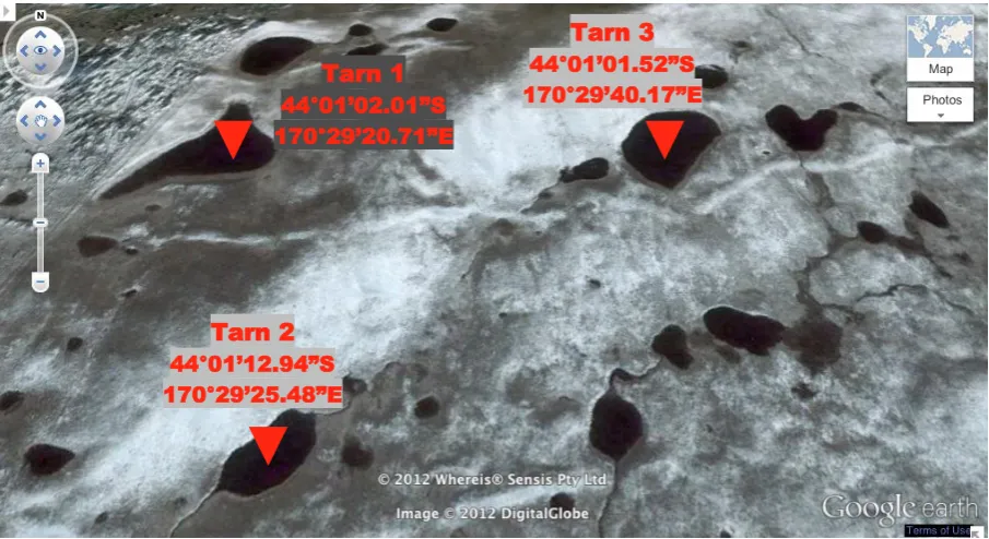
Figure 5. Location of tarns near Lake Tekapo, New Zealand.

Figure 6. Sample locations in the three tarns from which samples were collected. Each dot shows where water samples, and other data were collected.

Tarn 3 44°01’01.52”S 170°29’40.17”E Tarn 1

44°01’02.01”S 170°29’20.71”E

(25)

2.1.3 Sample collection

A custom designed sampling apparatus was constructed to allow the collection of samples

with minimal disturbance of the tarns while also being portable and easy to set up. The

sampling apparatus (Figure 7 & Figure 8) consisted of; (i) two adjustable support poles that

were erected either side of the tarns, (ii) a length of rope with tubing attached, connecting

the two poles together, (iii) a floatation device (Figure 9) that allowed the end of the tubing

to be positioned at a set depth of 5 cm below the water’s surface and finally (iv) a

petrol-engine pump which was used to transfer the water through the tubing. To ensure that each

sample was not contaminated with water from the previous sample, after the collection of

each sample, both ends of the tubing were briefly removed from the water to allow the

formation of an air bubble and then the tubing was flushed until approximately 10 seconds

after the air bubble had been expelled.

(26)

Figure 8. One of the support poles with attached rope and tubing of the sampling apparatus.

(27)

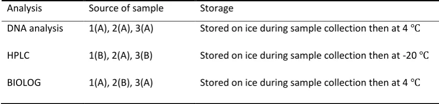
For Tarn 1, two 250 mL opaque sample bottles (1(A), 1(B)) were filled to capacity with water

for each sample (Table 1). Two 250 mL bottles (3(A), 3(B)) were also collected for Tarn 3. Due

to resource limitations, for Tarn 2, only one 250 mL bottle (2(A)) was collected per sample.

However, an additional 15 mL of water was collected in a centrifuge tube (2(B)) for each

sampling location in Tarn 2.

Table 1. Samples required for analyses and storage conditions.

Analysis Source of sample Storage

DNA analysis 1(A), 2(A), 3(A) Stored on ice during sample collection then at 4 ℃

HPLC 1(B), 2(A), 3(B) Stored on ice during sample collection then at -20 ℃

BIOLOG 1(A), 2(B), 3(A) Stored on ice during sample collection then at 4 ℃

2.1.4 Physicochemical properties of the tarns

A range of physicochemical properties were measured onsite. These included; pH, dissolved

oxygen, temperature and depth. To measure pH, 250 mL of water from each sample location

was collected in a measuring cylinder and the pH was recorded using a portable pH meter

(handylab pH 11, SCHOTT Instruments) within five minutes of sample collection. The

dissolved oxygen content and the temperature of the tarns were measured using a dissolved

oxygen probe (550A YSI, Yellow Springs, OH). The depths of the tarns were measured using a

pole marked at 5 cm intervals.A minimum of 12 random sites in each tarn were analysed for

the suite of physicochemical properties. Samples were also collected for chemical analysis.

These samples were analysed by High Performance Liquid Chromatography (HPLC), by Joy

Jiao, Lincoln University. HPLC allows the concentrations of various anions; chloride, bromide,

(28)

2.2 Molecular methods

2.2.1 Filtration procedure

In preparation for DNA extraction and subsequent analysis, water samples were filtered

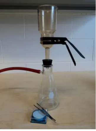
using a Buchner filter (Figure 10) to collect bacterial cells on filters.

Figure 10. Buchner filter showing a Buchner funnel (Nalgene®, Thermo SCIENTIFIC, Rochester, NY, U.S.A.) and the waste collection container (KIMAX®, KIMBLE, Vineland, NJ, U.S.A.).

Using a Buchner filter, 100 mL of each sample was filtered through a new filter (Millipore

Express® PLUS Membrane, polyethersulfone, hydrophilic, 0.22 µm, 47 mm, MERCK Millipore,

Billerica, MA, U.S.A.). Using sterile forceps the filter was placed in a bead beater tube (Micro

tube, 2 mL, Global Science and Technology, Auckland, New Zealand), containing 0.5 g of 0.1

mm zirconia/silica beads and 0.5 g of 2.3 mm zirconia/silica beads (BioSpec, Inc., Bartlesville,

OK, U.S.A.). The bead beater tubes were then stored in a freezer at -20 °C. After each sample

had been filtered, the filtering apparatus was rinsed with tap water and then distilled water.

The forceps were sterilised between each sample to avoid the transfer of contaminants by

(29)

2.2.2 DNA extraction

In order to investigate the microbial diversity in the tarns the DNA had to first be extracted

from the filters prepared in the previous procedure (see section 2.2.1). The DNA extraction

procedure utilised in this study was adapted from Miller et al. (1999). To extract the DNA,

270 µL of phosphate buffer (100 mM, pH 8.0) and 300 µL of Sodium Dodecyl Sulphate (SDS)

lysis buffer (100 mM, Tris pH 8.0, 10% SDS) were added to each bead beater tube containing

a filter. The samples were then gently mixed by hand and then 300 µL of chloroform:isoamyl

alcohol (24:1) was added to each tube. Tubes were shaken in a TissueLyser II (QIAGEN®,

bio-strategy, Auckland, New Zealand) at 3 m s-1 for 1 min. The tubes were then transferred to

the other side of the TissueLyser II and shaken for another minute. The tubes were

transferred to a bench top centrifuge (Spectrafuge 24D; Labnet, Woodbridge, NJ, U.S.A.) and

were centrifuged at full speed (13,300 rpm) for 5 min to pellet debris. The supernatant

(approximately 650 µL) was transferred to a clean 1.5 mL microtube (AXYGEN, Auckland,

New Zealand) and then 360 µL of 7 M ammonium acetate (NH4OAc) added to the tubes to

achieve a final concentration of 2.5 M. The tubes were gently mixed by hand and then

centrifuged at full speed (13,300 rpm) for 5 min. After centrifugation, two distinct phases

were observed, with the SDS forming a gel-like interphase. The upper phase (approximately

580 µL) was transferred to a clean 1.5 mL microtube and 315 µL of ice-cold isopropanol

(Analar) was added to each tube. The tubes were then incubated at room temperature for

15 min before centrifugation at full speed (13,300 rpm) for 5 min to pellet the DNA. The

supernatant was then discarded and the pellets were washed using 1 mL of 70% ethanol.

The tubes were again centrifuged at full speed (13,300 rpm) for 5 min and the supernatant

discarded. The pellets were then dried in a desiccator jar under vacuum for 15 - 45 min.

Once the pellets were dry, they were resuspended in 50 µL of Nuclease-Free water

(Promega, Sydney, Australia).

2.2.3 Polymerase chain reation (PCR)

PCR was performed on the DNA extracts to amplify bacterial DNA that was of interest to us

in the present study. The PCR that was performed utilised primers designed for automated

ribosomal intergenic spacer analysis (ARISA). ARISA primers (InvitrogenTM Ltd., Victoria,

(30)

16S rRNA and the 23S rRNA genes. This region is highly variable among different microbial

species and thus a PCR utilising ARISA primers will result in the production of many

fragments of different lengths. The resulting fragment pattern can therefore be used to

characterize differences in microbial community composition among samples. For the PCR, a

master mix containing all the different components required for a PCR was made (Table 2).

The GoTaq® reagent (Hot Start Green Master Mix, 2X, Promega, Sydney, Australia) used in

the master mix contained Taq DNA polymerase, dNTPs, MgCl2 and reaction buffers at

optimal concentrations.

Table 2. Reagents used to create a mastermix suitable for the PCR amplification of DNA for ARISA for one sample.

*SD Bact (5’-TGCGGCTGGATCCCCTCCTT-3’) (InvitrogenTM Ltd., Victoria, Australia)

** LD Bact (5’-CCGGGTTTCCCCATTCGG-3’) (InvitrogenTM Ltd., Victoria, Australia)

For each sample, 48 µL of master mix was added to each well of a 96 well plate (Scientific

Specialties Inc., Lodi, CA, U.S.A.) and then 2 µL of DNA extracts added to each well, except

for two DNA-free controls which were included to ensure that PCR mastermixes were not

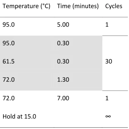
contaminated with bacterial DNA. PCR was performed in a thermal cycler (Veriti, 96 Well

Thermal Cycler, Applied Biosystems, Victoria, Australia) under the following conditions listed

in Table 3.

Reagent Volume

Nuclease-Free water 18 µL

*Forward primer, SD Bact (10 µM) 2 µL

**Reverse primer, LD Bact (10µM) 2 µL

Bovine serum albumin BSA, 10%

(InvitrogenTM Ltd., Victoria, Australia)

1 µL

GoTaq® (Hot Start Green Master Mix,

2X, Promega, Sydney, Australia)

25 µL

DNA (2 µL)

Total volume (master mix) 48 µL

(31)

Table 3. Conditions under which the PCR was performed.

Temperature (°C) Time (minutes) Cycles

95.0 5.00 1

95.0 0.30

61.5 0.30 30

72.0 1.30

72.0 7.00 1

Hold at 15.0 ∞

2.2.4 Agarose gel electrophoresis

Agarose gel electrophoresis was performed on the PCR samples to confirm that the DNA

extraction and PCR both worked. An agarose gel was prepared by combining 1.5 g of agarose

(AppliChem low EEO powder, Auckland, New Zealand) in 100 mL of 1X Tris/Borate/EDTA

(TBE) buffer in a 500 mL Schott bottle. The agarose was dissolved by heating in a microwave

for two minutes, or until fully dissolved. The liquid agarose was allowed to cool to the touch

before 10 µL of SYBR® safe DNA stain (invitrogen, Victoria, Australia) was added and then

the solution was poured into a rectangular gel mould and left to set at room temperature

(20 min). The solid agarose gel was placed into the electrophoresis apparatus (ENDURO,

Labnet, Woodbridge, NJ, U.S.A.) and 1X TBE was added until the gel was completely

submerged. The gel was then loaded with 6 µL of 1 Kb Plus DNA ladder (E-Gel®, invitrogen,

Victoria, Australia) into the first well. With the samples, 6 µL of each sample (including the

negative controls) was loaded directly into individual wells of the gel because the GoTaq®

master mix already contains loading dye. Electrophoresis was performed at 110 V for 30 to

40 min. The gel was then visualised under UV light using a gel doc (UVItec Limited,

(32)

2.2.5 DNA purification

The agarose gel electrophoresis confirmed that DNA was present in the samples and no

contamination was observed in the negative controls, therefore DNA purification was

performed. DNA was purified (using a DNA Clean & ConcentratorTM-5 Kit; ZYMO RESEARCH,

Irvine, CA, U.S.A.) to remove the primers and other unwanted DNA sequences in the

samples.

2.2.6 Automated ribosomal intergenic spacer analysis (ARISA)

After DNA purification had been performed 1 μl of each sample was combined with 10 μl

HiDi formamide and an internal LIZ1200 standard (Applied Biosystems Ltd., New Zealand).

The samples were then heat treated (95 °C, 5 min) and cooled on ice. To generate ARISA

profiles, the samples were run on a 3130XL Capillary Genetic Analyser (Applied Biosystems

Ltd.) using a 50 cm capillary and standard Genemapper protocol, but with an increased run

time (15 kV, 65 000 s).

2.3 Functional analysis (carbon substrate utilisation)

To provide a measure of the functional capability of the bacterial community in each sample,

BIOLOG EcoPlates™ (BIOLOG Inc, Hayward, CA, U.S.A., Figure 11) were inoculated by

aliquoting 120 µL of each sample into individual wells which contain a range of carbon

substrates (Appendix A). The plates were incubated in the dark, at room temperature, for

approximately 48 hours. The absorbance of the colour produced in the individual wells was

measured at a wavelength of 590 nm using a plate reader (BMG LABTECH FLUOstar Omega

model). The absorbance recorded for the well containing water was used as a blank and the

(33)

Figure 11. Unused BIOLOG EcoPlate™ (left) and BIOLOG EcoPlate™ (right) showing colour development.

2.4 Statistical analysis

GENEMAPPER software (v 3.7; Applied Biosystems Ltd.) was used to produce

electropherograms from the fluorescence data obtained during the ARISA procedure. The

electropherograms provide a comparison of the proportional quantities of different-sized

DNA fragments in each sampled community (Lear et al., 2008).The protocol of Ramette et

al. (2009) was then used to identify ‘true peaks’ (i.e., removing background ‘noise’ generated

during automated analysis) and bin fragments of similar size. Each number greater than

zero, in the tabulated ARISA data (Appendix B), represented a detected taxon. The ARISA

and BIOLOG data were standardised, in which relative percentages, disregarding the effect

of total abundance (ARISA) or intensity (BIOLOG) were calculated. A Bray-Curtis similarity

matrix (Legendre and Legendre, 1998) was then produced for both bacterial community

structure (ARISA data) and function (BIOLOG data) in PRIMER (version 6.1.12; Primer-E Ltd.,

Plymouth, UK) to allow a quantitative description of the relative differences among the

samples. The following Bray-Curtis equation was used to produce the matrices;

( ∑

∑ ∑ ), eq. 1

where is the standardised peak size of taxon i from sample 1 and is the standardised

peak size of taxon i from sample 2 (Clarke and Gorley, 2006). This was calculated for all

(34)

2.4.1 Evaluation of the taxa-area hypothesis

To determine whether positive taxa-area relationships existed in the tarns, a species

accumulation curve was plotted (using the tabulated ARISA data) for each tarn using the

‘exact’ argument (Kindt et al., 2006) in the ‘specaccum’ function in the ‘vegan’ package in R

(version 2.15.2) (R_Core_Team, 2012). A taxa-area curve usually involves species richness

being plotted against area sampled. However, with this study, the method that was used to

determine bacterial richness, ARISA, only has resolution to taxa (ARISA peak) level, not

species level, and therefore taxa richness was plotted instead of species richness. The

cumulative number of samples was used to represent sample ‘area’ because each analysed

sample was approximately the same volume of water (100 mL) (samples were taken

approximately 7 m apart from each other in a grid format). After the curves were plotted, a

power law function was fitted to the data using the non-linear regression function ‘nls’ in R

(version 2.15.2) (R_Core_Team, 2012) (see Appendix C for R script). For Tarn 3, the samples

collected from the smaller grid format of 3.5 x 3.5 m were excluded to allow a direct

comparison of these data with data collected from Tarns 1 and 2, from which such samples

were not collected.

2.4.2 Evaluation of the distance-decay hypothesis

Distance-decay plots were produced for both the ARISA and BIOLOG data. The ‘vegan’

package in R (version 2.15.2) (R_Core_Team, 2012) was used to calculate a Bray-Curtis

similarity matrix (see eq. 1) for both bacterial community structure (ARISA data) and

function (BIOLOG data). These similarity matrices were then used to compare similarity in

bacterial community data with their geographic (straight-line) distance apart. For Tarn 3, the

samples that were collected from the smaller grid format of 3.5 x 3.5 m were included in the

analysis to increase the sensitivity of the approach. For bacterial community structure an

exponential curve was fitted to the data using the non-linear regression function ‘nls’ in R

(version 2.15.2) (R_Core_Team, 2012). The function took the form, , where S

is the pairwise Bray-Curtis similarity, a is a constant and distance is pairwise distance. A

linear function was fitted to the data for bacterial community function (see Appendix D for R

(35)

2.4.3 Evaluation of the space vs environment hypothesis

Variation among the tarns

Using PRIMER (version 6.1.12; Primer-E Ltd., PERMANOVA+ add on, Plymouth, UK), the

overall variation in the tarns was visualised by producing non-metric multi-dimensional

scaling (MDS) plots. Two-hundred and fifty re-starts were conducted for both bacterial

community structure and function using the respective Bray-Curtis matrix. MDS plots are 2-d

or 3-d ordination plots in which the relative distances apart of all points are in the same rank

order as the relative Bray-Curtis similarities of the samples. This results in samples that have

more similar bacterial community structure or function being located closer together.

Permutational MANOVA (PERMANOVA) was then performed to determine if there were

significant differences in bacterial community structure and function among the tarns, and

to identify the tarns with the most similar/dissimilar communities. Type III (partial) analyses

with 9999 unrestricted permutations of the raw data were used (Lear et al., 2008). Like the

more traditional, multivariate analysis of variance (MANOVA), PERMANOVA is used to

determine if the means of several groups are significantly different. The advantages of using

PERMANOVA over MANOVA are that PERMANOVA can be used for unequal group sizes and

also, because PERMANOVA is a permutation method, it is unaffected by the statistical

distribution of the samples.

To visualise spatial differences in bacterial community structure and function among the

tarns, contour plots of the data were constructed for each study site. The values plotted on

the contour plots were the 1-d ‘configuration scores’ sourced from the MDS plots of the

ARISA and BIOLOG Bray-Curtis for all tarns. The data from the contour plots were

interpolated using the inverse distance weighting (IDW) interpolation function in the

Geostatistical Wizard, ArcMap10 (Esri, Wellington, New Zealand). The IDW function predicts

values for unmeasured locations by using measured values surrounding the prediction

locations. More weight is given to values close to the prediction locations than values that

are further away. After the predicted values had been calculated, the range of values were

classified into ten even classes and each class was assigned a colour from a colour gradient

(lowest value = dark blue to highest value = light green) with more similar colours

representing more similar values. Similar plots were produced by Jones at al. (2012) (see

(36)

which sampling locations that contained similar bacterial communities were represented by

a similar colour.

Differences in environmental variables among the three tarns were determined by

calculating the mean concentration and standard error of each environmental variable (pH,

conductivity, total carbon, chloride, nitrite-N, bromide, nitrate-N, phosphate-P, sulphate-S)

and performing Tukey’s test in MiniTab 16 to confirm significant differences (P ≤ 0.05).

Tukey’s test identifies means that are significantly different by comparing all possible pairs of

means.

Variation within the tarns

The following analyses were all performed in PRIMER (version 6.1.12; Primer-E Ltd.,

PERMANOVA+ add on, Plymouth, UK). An MDS plot was produced for each tarn, based on a

resemblance matrix constructed from Bray-Curtis similarity data. For the same sample data a

cluster diagram, or dendogram was plotted using the ‘group average’ approach. Bacterial

samples that were determined to be less than or equal to 50 % similar using this approach

were then marked as separate clusters on the MDS plots. Clusters were not overlaid on the

MDS plots for bacterial community function because all the samples for each tarn were

constrained in one cluster at the 50 % similarity level (Appendix E). The significant

differences in bacterial community structure among the clusters were investigated using

PERMANOVA (type III (partial), unrestricted permutation of raw data, 9999 permutations).

The total variation in bacterial community structure among the samples within each tarn

was analysed using the multivariate dispersion (MVDISP) function which calculates a factor

dispersion value in which larger values are indicative of greater variation in the samples. The

clusters were plotted on maps of each tarn (where different data clusters were represented

by different colours) allowing the visualisation of the position of the clusters within the

tarns. The same approach that was used to produce the contour plots showing the variation

among the tarns (see section 2.4.3; ‘Variation among the tarns’) was used to produce

contour plots for both bacterial community structure and function within the individual

tarns, using the ARISA and BIOLOG Bray-Curtis data for the individual tarns to identify any

(37)

To analyse the environmental variation in the tarns, regression analyses were performed

using distance-based linear models (DistLM) as used by Lear et al. (2008) to identify any

environmental variables that had a significant relationship with bacterial community

structure or function after any correlated environmental variables (Draftsmans plot,

r < -0.05; r > 0.05) had been removed. DistLM was carried out using the following

parameters in the Primer-E program: selection procedure; ‘Forward selection’, which adds

one variable, the variable that improves the selection criterion the most, at each step until

no improvement in the selection criterion is possible; selection criteria, ‘ R2’, which is the

proportion of explained variation and finally 9999 permutations were performed. DistLM is a

regression analysis that models the relationship between a resemblance matrix (e.g.

Bray-Curtis similarity matrix) and a set of predictor variables, which in this study were a range of

environmental variables. For any environmental variable that was identified as having a

significant relationship with bacterial community structure or function, the IDW

interpolation function in the Geostatistical Wizard, ArcMap10, was used to produce a

contour plot from the raw data for the environmental variable. This allowed the visualisation

of any spatial patterns present in these environmental variables in the tarns.

Finally, variance partitioning was performed using DistLM to determine the proportion of

total variation explained by either spatial location, environment variables or a combination

of both for each tarn separately. The spatial factors and environmental variables were

divided into two categories using the ‘Indicator’ function in PRIMER (version 6.1.12; Primer-E

Ltd., PERMANOVA+ add on, Plymouth, UK). One of the categories, Space (S) consisted of the

complete trend surface regression (Eastings (E), Northings (N), E2, N2, EN, E2N, N2E, E3, N3)

(Legendre and Legendre, 1998)and the other category, Environment (E) included any

uncorrelated (see section 2.4.3 ‘Variation within tarns’) environmental variable data. DistLM

analysis was carried out using the following parameters in the Primer-E program: Group

variables (S and E); selection procedure; ‘All specified’, which fits the predictor variables (S

and E) in the order given under the ‘Force inclusion’ column in the ‘Selection’ dialog, ‘R2’ and

finally 9999 permutations were performed. Dividing the data into two categories, S and E,

allowed the proportion of total variation explained by one of these categories to be

determined directly from the DistLM output. This value was used to manually calculate the

proportion of total variation explained by the other category and space and environment