Spatiotemporal Dynamics of Neural Activity During Human Episodic Memory Encoding and Retrieval

University of Pennsylvania

ScholarlyCommons

Publicly Accessible Penn Dissertations

1-1-2014

Spatiotemporal Dynamics of Neural Activity

During Human Episodic Memory Encoding and

Retrieval

John Frederick Burke

University of Pennsylvania, [email protected]

Follow this and additional works at:http://repository.upenn.edu/edissertations

Part of theNeuroscience and Neurobiology Commons

This paper is posted at ScholarlyCommons.http://repository.upenn.edu/edissertations/1218

Recommended Citation

Burke, John Frederick, "Spatiotemporal Dynamics of Neural Activity During Human Episodic Memory Encoding and Retrieval" (2014).Publicly Accessible Penn Dissertations. 1218.

Spatiotemporal Dynamics of Neural Activity During Human Episodic

Memory Encoding and Retrieval

Abstract

Throughout literary history, the ability to travel in time has been a source of wonder and amusement. Why this fascination with moving through time? One reason may be that people are especially attuned to the concept of time travel because we each possess our own personal mental time machine: episodic memory. Through episodic memory, we transport ourselves back in time to re-live experiences from our past. This allows us to reflect on our own self-knowledge, effectively placing ourselves in context of our lives. This dissertation investigates how our brains accomplish this highly sophisticated cognitive operation. Using a laboratory model of episodic memory (free recall) and a particularly powerful neuroimaging tool (intracranial EEG), I document the changes that occur in the brain as episodic memories are first formed and then later retrieved. I find that the episodic memory system is best conceptualized as stage-wise process consisting of distinct brain regions that activate at highly conserved times relative to memory formation/retrieval. These discrete activations are used to construct a novel neurological model of episodic memory, the Neurological Stages of Episodic Retrieval and Formation (N-SERF) model. Future work should be aimed at verifying the hypotheses put forward by the N-SERF model, we well as relating the N-SERF model to prominent computational models of episodic memory.

Degree Type Dissertation

Degree Name

Doctor of Philosophy (PhD)

Graduate Group Neuroscience

First Advisor Michael J. Kahana

Keywords

EEG, Episodic memory, gamma, theta

Subject Categories

SPATIOTEMPORAL DYNAMICS OF NEURAL ACTIVITY DURING HUMAN

EPISODIC MEMORY ENCODING AND RETRIEVAL

John F. Burke

A DISSERTATION

in Neuroscience

Presented to the Faculties of the University of Pennsylvania in Partial

t of the Requir s for the Degree of Doctor of Philosophy

2014

Michael J . Kahana, Ph.D. Supervisor of Dissertation

Joshua Gold, Ph.D.

Graduate Group Chairperson

Geoffrey K. Aguirre, M.D., Ph.D. David H. Brainard, Ph.D.

Nicole C. Rust, Ph.D. Karee A. Zaghloul, M.D., Ph.D.

Associate Professor RRL Professor

Professor Associate Professor

Assistant Professor Adjunct Assistant Professor

Acknowledgments

First, I would like to thank the 100+ people with intractable epilepsy who have graciously volunteered their time to participate in this study. I had the opportunity to meet some of these patients. They often told me that they were motivated to participate in memory testing simply because they wanted to help others. Their selflessness is a source of inspiration.

I would like to thank my advisor, Michael J. Kahana. In the last decade, Mike has fostered my professional and scientific development and has been a dedicated and selfless mentor. One thing Mike taught me (or at least tried to teach me) was to eliminate the flu↵ from my writing and to communicate specific and precise ideas. With that in mind, Mike possesses two specific characteristics for which I am particularly grateful. First, he has a passion for studying how we remember. His love of memory drives the CML, and if anything I found in my research taught him something new about memory, then my time in lab was a success. Second, his scientific instincts are uncanny. He always knows what to do next, when to stop, when to push ahead (and he is always dead right!). Mike is a great mentor, a fantastic leader, and a close friend.

model of how a neurosurgeon could successfully participate in research. Kareem is a great friend and a great surgeon.

I would like to thank my committee members, Drs. Geo↵rey Aguirre, Nicole Rust, and David Brainard for their support, guidance and ideas throughout my training.

ABSTRACT

SPATIOTEMPORAL DYNAMICS OF NEURAL ACTIVITY DURING HUMAN EPISODIC MEMORY ENCODING AND RETRIEVAL

John F. Burke

Michael Kahana, Ph.D.

Contents

Acknowledgments ii

Abstract iv

Contents v

List of tables vii

List of figures viii

1 Introduction 1

1.1 Episodic memory in the laboratory: Free recall . . . 3

1.2 Assaying brain activity: intracranial EEG . . . 6

1.3 Overview . . . 10

2 Synchronous and asynchronous theta and gamma activity during episodic memory formation 13 2.1 Abstract . . . 13

2.2 Introduction . . . 14

2.3 Methods . . . 16

2.4 Results . . . 29

3 Human intracranial high-frequency activity maps episodic memory

for-mation in space and time 48

3.1 Abstract . . . 48

3.2 Introduction . . . 49

3.3 Methods . . . 51

3.4 Results . . . 56

3.5 Discussion . . . 63

4 Theta and high-frequency activity mark spontaneous episodic retrieval during free recall 73 4.1 Abstract . . . 73

4.2 Introduction . . . 74

4.3 Methods . . . 76

4.4 Results . . . 81

4.5 Discussion . . . 94

5 General discussion 100 5.1 Contributions of this dissertation . . . 100

5.2 Electrophysiology of memory encoding and retrieval . . . 101

5.3 The neurological stages of episodic retrieval and formation (N-SERF) model . . . 105

5.4 Brain computer interface (BCI) experimental paradigm . . . 110

5.5 Stimulation experimental paradigm . . . 116

5.6 Concluding remarks . . . 119

List of tables

2.1 Patients included in all studies. . . . 19

3.1 Pairwise tests of timing di↵erences between left-hemispheric

regions-of-interest . . . 62

4.1 Number of patients and electrodes contributing to each anatomical

region. . . . 78

List of figures

1.1 Early descriptors of episodic memory . . . 2

1.2 Free recall task . . . 4

1.3 Intracranial electroencephalography . . . 8

2.1 Bipolar electrode montage . . . 23

2.2 Change in theta and gamma power across anatomical location . . . 30

2.3 Temporal evolution of changes in theta and gamma power . . . 32

2.4 Examples of theta and gamma power fluctuations during success-ful memory formation . . . 33

2.5 Change in theta and gamma lobe-wise synchrony during memory encoding . . . 35

2.6 Aggregating pair-wise network connections . . . 37

2.7 Change in theta and gamma degree across anatomic locations . . . 39

2.8 Temporal evolution of changes in theta and gamma degree . . . 41

3.1 Spectral specificity of power changes during encoding (0-2000 ms post word presentation) . . . 58

3.2 Anatomical specificity of power changes during encoding (0-2000 ms post word presentation) . . . 59

3.4 Timing comparisons of HFA between regions-of-interest (ROIs) . . 64

3.5 Regions clustered by temporal activation profile . . . 66

4.1 Retrieval dynamics in epileptic patients and healthy volunteers . . 82

4.2 Spectral activity during retrieval . . . 84

4.3 High-frequency activity (HFA; 64–95 Hz) across time during retrieval 86 4.4 Theta activity (3–8 Hz) across time during retrieval . . . 87

4.5 Spectral activity during vocalization . . . 89

4.6 Timing of theta and HFA across regions-of-interest (ROIs) . . . 91

4.7 Examples of changing theta and HFA dynamics in the right tem-poral lobe . . . 93

4.8 Right temporal lobe spectrograms during retrieval . . . 94

5.1 Recording unit activity during free recall task . . . 104

5.2 The Neurological Stages of Episodic Retrieval and Formation (N-SERF) model . . . 106

5.3 Brain Computer Interface Overview . . . 112

5.4 BCI implementation . . . 114

5.5 Memory stimulation experimental paradigm . . . 117

Chapter 1

Introduction

In the 1913 novel “In Search of Lost Time”, Marcel Proust describes a memorable scene that is often simply referred to as theEpisode of the Madelaine(Proust, 1913). The Madeleine refers to a small cake that is characteristic to a particular region of France (Figure 1.1A). The protagonist in the scene, upon tasting a Madeleine cake for the for the first time in many years, is overcome with a sudden change in his thoughts, emotions, and overall internal mental state. Initially, he struggles to define the change that has occurred. Given that nothing peculiar has happened in the environment around him, he reasons that this powerful force must have originated from inside of his head. But where? And, how? Soon, and with conscious mental e↵ort, he is able to identify what change has overcome him: he has retrieved an episodic memory.

A

B

Figure 1.1: Early descriptors of episodic memory.A: The Madeleine cake that was the inspiration

for Proust’s famous episode.B: Endel Tulving, the first to formalize the concept of episodic memory in a scientific framework.

Indeed, given the correct cue (the Madeline cake) and conscious mental e↵ort, he was able to travel back in time to re-experience a personal episode

Five decades later, episodic memory was formally described by Endel Tulving (Tulving, 1972) (Figure 1.1B). In his view, episodic memory involved remembering personal experiences as opposed to rote facts. Tulving noted that episodic mem-ory is accompanied by a feeling of “mental time travel” (Tulving, 1983). Once formalized in this manner, it is trivial to recognize the episode of the Madeleine as particularly salient example of the retrieval of an episodic memory. Indeed, every person has similar examples from his or her own life—such memories form the building blocks of our own personal history.

scien-tific intrigue, understanding the neural substrate of episodic memory will also help us more adequately treat pathological processes that disproportionately af-fect episodic memory, most notably Alzheimer’s disease and the cognitive decline that accompanies aging, which carry an enormous social cost (Hurd, Martorell, Delavande, Mullen, & Langa, 2013).

This dissertation is driven by a desire to more completely understand how the brain supports episodic memory formation and retrieval. In e↵ect, we can imagine ourselves as Proust the scientist. Instead of writing a novel, we will instead attempt to follow an episodic memory through the brain, from its initial formation until its ultimate retrieval. In order to accomplish this, we will need two laboratory tools. First, we need a method to simulate episodic memory formation and retrieval in a shortened amount of time, so we can observe both processes in the research setting. Second, we need a way to assay brain activity. Each of these important methodological considerations are briefly summarized in the following two sections.

1.1 Episodic memory in the laboratory: Free recall

It may seem difficult to recapitulate the formation and subsequent retrieval of episodic memories in the laboratory setting. How is it possible to induce people to engage in mental time travel? And, more importantly, how could one reliably determine if such mental time travel actually took place?

Time CAR FLAME FENCE PASTE PEN 9+7+3 1+9+19+7+3_{8+6+39+7+33+5+99+7+3}

6+2+29+7+3₂₊₈₊₁

Encoding P eriod Distr actor Recall P eriod CAR FENCE PEN

A

B

0 20 40 60 80 100

0 ms 1600 ms 2400 ms + JITTER

CAR FLAME List Number Time (sec) Session 1 Session 2 Session 3 Session 4 Orient Cue Recalled Word Not- Recalled Word

Vocalization Intrusion (extra-list) Start of Recall

Repeated item Intrusion (prior-list) 1 2 3 4 5 6 7 8 9 10 1 2 3 4 5 6 7 8 9 10 1 2 3 4 5 6 7 8 9 10 1 2 3 4 5 6 7 8 9 10

Encoding Period Distractor Recall Period

0 -4 -2 2 4 5

0.04 0.06 0.08 0.1 0.12 0.14 0.16 0.18 0.2 0.22 0.24 -1 -3

-5 1 3

Response P

robabilit

y

Temporal Transition (lag)

C

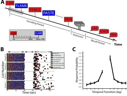
Figure 1.2: Free recall task. A: In the delayed free recall task, participants are given a list of words,

and are then asked to retrieve/vocalize the words in the most recent list.B: Example behavioral data from one participant across four sessions of delayed free recall. A trial began with an orientation cue (green squares); a list of words was then presented, one after the other (red and blue circles during encoding). After a 20 sec distraction task, the patient was asked (black star) to recall as many words as possible from the list in any order. Words recalled from the most recent list were considered correct retrievals (red circles). Recalled words that were not on the most recent list were intrusions, which were either presented to the patient in a previous list (prior-list intrusions; yellow-circles) or not presented to the patient at all (extra-list intrusions; gray-circles).C: Given a word from a certain list position was retrieved, the probability (y-axis) that the next retrieval was from a word from a nearby list position (lag; x-axis). Errorbars represent_±1 SEM across 98 patients.

period. During a typical test, a person may be shown 10 or more such lists in one sitting, allowing the experimenter to collect a sufficient amount of data to thoroughly investigate the person’s memory performance (Figure 1.2B).

which recognition memory is a special case), cued recall, autobiographical recall, etc. However, free recall is a particularly powerful method to study episodic mem-ory because the recall portion is unconstrained, placing an emphasis on internal memory search (Kahana, 2012). Specifically, by carefully studying how partici-pants transition from one retrieval to the next, it is possible to infer how a person is searching through their memory (Polyn, Norman, & Kahana, 2009). Using this technique, it has been shown that participants tend to search their memory based on how close in time that items were presented duringencoding. This finding, termed the law of contiguity (Kahana, 1996), suggests that participants jump backward in time (after retrieving an item) to the time period when the item was first presented. Once the participant has mentally travelled back in time in this manner, they are then more likely to recall words that were presented surrounding the original item (Figure 1.2C).

1.2 Assaying brain activity: intracranial EEG

There are many methods to assay brain activity during a cognitive task. One of the earliest methods, scalp electroencephalography (EEG), involved placing an elec-trode on the surface of the skull, and recording the voltage di↵erence between that electrode and a neutral reference electrode. Indeed, the first electrophysiological correlate of human behavior was found using this method (H. Berger, 1929). Later studies similarly recorded scalp EEG during other behaviors, such as memory tasks. These studies examined the amplitude/potential of the recorded EEG signals during the encoding of items, and compared the EEG amplitudes recorded during items that were later recalled versus later not recalled (Sanquist, Rohrbaugh, Syn-dulko, & Lindsley, 1980)1_{. Based on these “event related potentials” (ERP), these}

studies could thus infer which areas of the brain were, in general, active during the formation of a memory. A similar method was used to investigate which ar-eas were active during episodic memory retrieval (Rugg & Wilding, 2000; Curran, 2000; M. D. Rugg & Curran, 2007).

Orthogonal to the aforementioned studies of episodic memory, scalp EEG has been used in the clinical setting to diagnose epilepsy for many decades (Engel Jr & Pedley, 2008). Epilepsy is a disease characterized by periodic and uncontrolled seizure activity that a↵ects over three million people in the United States2. In roughly one in four cases of epilepsy, traditional pharmacological interventions fail to control or stop seizures from occurring, and such patients are candidates for a procedure in which an area of the brain is surgically removed (J. J. Engel, 2001). Ideally, the resected brain area is responsible for seizure generation and

1_{This analysis was referred to as the di↵erence in memory (Dm) e↵ect and, later, as the} subse-quent memory (SM) e↵ect (Paller & Wagner, 2002). SM analyses are the most common method to

supports no other cognitive function. This theoretical brain area is referred to as the epileptogenic zone (L ¨uders, Najm, Nair, Widdess-Walsh, & Bingman, 2006). Even though the epileptogenic zone may only be partially realized in a patient’s brain, if the resected tissue sufficiently approaches the idealized epileptogenic zone, surgical intervention may be curative. Thus, a large emphasis is placed on finding the putative epileptogenic zone for every given patient. In order to accomplish this, scalp EEG is recorded continuously for many days in order to capture the onset of a seizure. If the seizure can be localized with a high degree of accuracy using scalp EEG, then the patient proceeds to surgery.

electrolim-A

P

I

S

C

5 subjects 30 subjects

A

B

Figure 1.3: Intracranial electroencephalography. A: Patients with pharmacologically resistant

activity without the typical signal loss through the skull, and thus has spatial res-olution on par with functional imaging studies. Critically, iEEG also maintains the very high temporal resolution of scalp EEG. Thus, iEEG maximizes neural infor-mation on a spatiotemporal scale, and is a very powerful tool to assay brain activity (A. K. Engel, Moll, Fried, & Ojemann, 2005; Jacobs & Kahana, 2010).

The typical procedure during intracranial monitoring for seizure localization (also referred to as phase II monitoring) is that the surgeon places electrodes beneath the patient’s dura mater (Figure 1.3A). The patient is then allowed to rest overnight, after which the required post-operative imaging is obtained (Figure 1.3B), and the patient is then “hooked-up” to the clinical amplifier and iEEG is recorded. iEEG is recorded continuously for a period ranging from 3 days to 2 months. During this time, the patient often sits idly on the epilepsy monitoring unit, watching television, reading books, receiving visitors, etc. As soon as the physicians feel that they have recorded a sufficient number of seizures to properly localize the epileptogenic region, the patient proceeds to surgery.

iEEG has the potential to aid both memory researchers and epileptologists alike. However, whereas epileptologist have leveraged iEEG for many decades for seizure localization (Crandall, Walter, & Rand, 1963), memory researchers have only recently begun to realize the power of iEEG to localize memory phenomenon (Fernandez et al., 1999; Fell et al., 2001; Sederberg, Kahana, Howard, Donner, & Madsen, 2003). More specifically, as patients with intracranial electrodes wait for seizures to occur, they may participate in research oriented, cognitive testing. In this way, iEEG can be safely and ethically recorded during memory tasks (Jacobs & Kahana, 2010). In this study, we take this approach and ask patients to perform

16 lists of a free recall task (Figure 1.2B). As mentioned previously, this task allows the episodic memory system to be observed in the laboratory setting. Therefore, by recording iEEG from epilepsy patients during free recall, it is possible to observe, with unmatched spatiotemporal resolution, the neural changes that occur during the formation and retrieval of episodic memories. In addition, because we have collected data from a large number of patients (Figure 1.3C), we can assess the activity in many di↵erent brain regions.

1.3 Overview

In summary, episodic memory is not simply an academic concept. It represents the uniquely human ability to re-live previous experiences, and has been documented by artists, scholars, and philosophers long before it was scientifically formalized. Episodic memory forms the building blocks of self-knowledge and consciousness of our own personal history (Tulving, 2002). It is often characterized by “mental time travel” and can be reproduced in the laboratory setting using tests of memory, particularly a free recall test. Uncovering the the neurological underpinnings of episodic memory is the first step toward (1) developing better therapies to treat the pathological decline of episodic memory and (2) sparing episodic memory function when planning neurosurgical procedures. One way to investigate the neural basis of episodic memory is to record iEEG from epileptic patients performing a free recall task. iEEG maximizes spatiotemporal information in human neural recordings, and can be used to trace an episodic memory in the brain from its formation until its ultimate retrieval.

propose a model of episodic memory based on the spatially and temporally discrete activations that occur during encoding and retrieval. This model, the Neurological Stages of Episodic Retrieval and Formation (N-SERF) model, suggests that these activation patterns represent a dynamic superposition of functional networks that collectively give rise to episodic memory. In the following chapters, I present three papers in support of this model, and synthesize these findings in the final chapter of the dissertation.

Chapter 2 presents a paper that examines the nature of the information that can be extracted from intracranial EEG data. Traditionally, scalp studies focused less on the localization of the brain regions responsible for episodic memory, and in-stead isolated particular oscillatory frequency bands that co-varied with particular mnemonic states (Nyhus & Curran, 2010). Indeed, entire theories regarding the neural mechanism of episodic memory are centered on the fact that oscillations in EEG co-vary with a variety of memory phenomenon (Fries, 2009; D ¨uzel, Penny, & Burgess, 2010; Fell & Axmacher, 2011). However, more recent work has suggested that EEG activity, especially in the high-frequency band, represents asynchronous, non-oscillatory changes (Miller, Sorensen, Ojemann, den Nijs, & Sporns, 2009). Because these two signals have vastly di↵erent implications about the types of information that can be extracted from EEG, this first chapter is devoted to deter-mining which of these processes, oscillatory vs. non-oscillatory, predominates in iEEG data during memory formation.

about memory formation is encoded by the time and location of spectral activity, and not the existence of spectral activity. This is the approach taken in this chapter. In Chapter 4, I use a similar strategy to understand the spatiotemporal pattern of activations that constitute episodic retrieval. In particular, I find that retrieval can be understood through a series of three electrophysiologically distinct stages relative to the onset of recall, and each stage has a unique spatiotemporal (and spectral) fingerprint. I relate each of these three stages to a prominent psychological framework of episodic memory, which o↵ers standardized concepts and novel insight into the electrophysiological correlates of retrieval.

Chapter 2

Synchronous and asynchronous theta

and gamma activity during episodic

memory formation

John F. Burke, Kareem A. Zaghloul, Joshua Jacobs, Ryan B. Williams, Michael R. Sperling, Ashwini D. Sharan, and Michael J. Kahana (2013).

The Journal Neuroscience, 33(1), 292–304.

2.1 Abstract

found that many key regions that showed power increases during successful mem-ory encoding also exhibited decreases in global synchrony. Similarly, cortical theta activity that decreases during memory encoding exhibits both increased and de-creased global synchrony depending on region and stage of encoding. We suggest that network synchrony analyses, as used here, can help to distinguish between two major types of spectral modulations: 1) those that reflect synchronous engage-ment of regional neurons with neighboring brain areas and 2) those that reflect either asynchronous modulations of neural activity or local synchrony accompa-nied by global disengagement from neighboring regions. We show that these two kinds of spectral modulations have distinct spatiotemporal profiles during memory encoding.

2.2 Introduction

Studies examining the electrophysiological correlates of memory encoding have demonstrated power fluctuations in theta (3–8 Hz) and gamma (>40 Hz) frequency bands that reliably co-vary with episodic memory formation (Kahana, 2006; Nyhus & Curran, 2010). One interpretation of these changes in spectral power is that they reflect oscillatory activity that mediates memory formation through phase synchronization (Axmacher, Mormann, Fern`andez, Elger, & Fell, 2006; Jensen, Kaiser, & Lachaux, 2007; Jutras & Bu↵alo, 2010; Fell & Axmacher, 2011).

Russeg-ger, & PachinRusseg-ger, 1996; M¨olle, Marshall, Fehm, & Born, 2002; Sederberg et al., 2003; Hanslmayr et al., 2011; Lega, Jacobs, & Kahana, 2011), memory encoding is also associated with an extensive decrease in theta power (?, ?; Guderian, Schott, Richardson-Klavehn, & Duzel, 2009). Second, the observed increases in gamma power during successful memory encoding occur across a wide range of frequen-cies extending from 30 to 100 Hz (Sederberg et al., 2007b). Such broadband activity is inconsistent with a mechanism that relies on precise narrow-band phase syn-chronization (Ray & Maunsell, 2010). An alternative hypothesis that has gained traction outside of the memory literature is that the observed increases in gamma activity often reflect an arrhythmic and intrinsically asynchronous process (Miller, Zanos, Fetz, den Nijs, & Ojemann, 2009; Manning, Jacobs, Fried, & Kahana, 2009; Ray & Maunsell, 2011).

Donner, & Engel, 2012).

Here, we use recordings from intracranial electrodes implanted in 68 partici-pants engaging in a free-recall task to simultaneously investigate changes in spec-tral power and phase during successful and unsuccessful memory encoding. We use a region-of-interest approach and a graph-theoretic metric of phase synchrony to localize both oscillatory and asynchronous activity in order to interpret the ob-served changes in spectral power. We find specific time intervals and anatomical locations that exhibit changes in both theta and gamma synchrony during mem-ory formation. By separating phase-synchronous oscillations from asynchronous changes, our results help clarify the role of rhythmic neural activity in the memory system.

2.3 Methods

2.3.1 Participants

Hosp ID Sex Age FSIQ #Sess LL #Items %Rec %PLI %ELI #BPE Lang Domin

BW

1 F 33 — 1 20 300 18.3 8.7 4.0 71 Left

2 F 51 — 1 20 300 22.0 2.7 0.3 35 Left

3 M 32 — 3 15 585 36.2 1.0 1.2 28 Left

4 M 40 — 2 15 285 28.8 12.6 10.5 116 Left

5 M 44 — 2 15 300 19.3 3.7 6.7 14 Left

6 M 26 — 2 15 300 25.3 3.0 2.0 96 Left

CH

1 F 13 — 1 20 240 24.6 0.8 0.4 88 Left

2 F 12 — 1 20 300 13.0 0.0 0.7 163 Left

3 M 15 — 3 20 600 15.0 1.7 1.7 184 Right

4 M 17 — 3 20 900 19.8 2.4 2.4 88 Left

5 M 15 — 1 20 300 28.7 2.0 1.0 200 Left

6 M 11 — 2 20 600 17.3 0.3 0.5 171 Right

7 F 14 — 1 20 300 34.7 2.3 1.7 95 Left

8 F 8 — 2 20 600 26.5 2.8 1.8 99 Left

9 M 17 — 1 20 280 10.7 3.2 4.3 105 Left

10 F 20 — 2 15 360 31.7 2.5 1.1 184 Left

11 M 14 — 3 15 450 20.9 2.9 4.0 128 Left

12 F 19 — 2 15 255 18.4 3.1 1.2 172 Left

13 M 16 — 1 15 240 31.7 1.7 0.4 232 Left

14 M 12 — 2 15 300 17.3 3.0 9.3 116 Right

15 M 13 — 4 15 600 33.3 0.5 0.5 103 Left

FR

1 M 33 — 1 20 180 23.9 0.0 0.0 108 Left

2 M 25 — 1 20 180 25.0 0.6 1.1 131 Left

3 M 31 95 1 20 180 13.3 2.2 0.0 72 Left

4 F 41 93 1 20 140 16.4 8.6 2.1 110 Left

5 F 34 — 1 20 140 27.1 3.6 2.1 42 Left

6 F 45 — 1 20 160 16.9 12.5 1.9 152 Left

7 F 46 85 1 20 300 16.7 2.0 2.3 20 Left

8 M 20 86 1 20 300 14.0 2.0 0.7 124 Left

9 F 53 104 1 20 300 16.3 7.0 7.0 44 Left

10 M 50 112 2 20 600 19.3 6.0 2.5 90 Left

11 M 28 86 1 20 300 12.3 0.3 0.3 171 Left

12 F 30 112 1 20 300 22.3 3.3 0.7 67 Right

13 F 37 90 1 15 300 21.7 24.3 14.0 39 Left

14 M 18 124 1 15 300 40.3 4.0 4.3 34 Left

15 M 23 97 4 15 1050 34.5 4.0 2.9 77 Left

16 M 21 94 1 15 150 32.7 6.7 2.0 144 Left

17 F 28 81 1 15 150 24.0 2.7 4.0 86 Right

18 F 35 100 2 15 300 18.0 2.0 2.0 181 Left

19 F 37 107 4 15 525 30.7 5.5 5.3 69 Left

20 M 19 98 2 15 450 35.1 3.6 1.8 96 Left

21 F 41 92 1 15 225 8.4 1.8 1.3 44 Left

22 F 21 82 1 15 225 22.2 1.3 1.8 112 Left

23 F 43 130 1 15 225 10.2 4.9 4.0 65 Left

24 M 19 104 2 15 375 32.0 1.3 1.6 44 Left

25 M 21 104 5 15 915 51.7 1.0 1.9 59 Left

26 F 35 104 1 15 225 19.6 7.1 7.6 87 Left

27 M 25 112 2 15 450 32.2 0.7 0.4 134 Left

28 M 47 112 1 15 225 26.2 5.8 6.7 88 Right

29 F 41 112 1 15 150 28.7 2.0 0.0 92 Left

TJ

1 M 25 100 3 15 720 32.2 0.8 0.1 60 Left

2 F 40 93 4 15 960 17.1 4.4 5.7 88 Left

3 M 39 100 1 15 240 22.1 3.3 8.3 43 Right

4 F 34 105 7₃ 15₁₅ 1680_{630 22.7}22.0 5.4_{1.9 1.1}1.5 ₉₅81 Left

5 M 44 111 1 15 195 15.9 3.6 3.1 110 Left

6 M 43 113 4 15 960 24.2 6.9 3.5 68 Left

7 M 21 89 3 15 720 20.1 3.3 7.6 129 Left

8 M 56 116 3 15 720 16.7 11.0 8.6 43 Left

9 F 57 88 2 15 420 10.0 3.6 9.0 81 Left

10 M 20 105 1 15 240 24.6 2.1 4.2 139 Left

1 15 240 28.3 0.4 0.8 50

1 15 150 26.7 1.3 1.3 139

Hosp ID Sex Age FSIQ #Sess LL #Items %Rec %PLI %ELI #BPE Lang Domin

TJ

11 M 41 97 2 15 480 20.8 3.8 1.2 84 Left

12 F 34 68 4 15 765 26.7 3.8 1.8 95 Left

13 F 52 106 1 15 240 36.7 0.8 1.2 95 Left

14 M 44 112 3 15 720 45.0 6.0 4.9 92 Left

15 M 33 123 4 15 960 32.0 2.0 1.7 105 Left

16 F 23 100 4 15 435 29.2 2.3 1.1 109 Left

17 F 48 88 2 15 480 35.0 5.2 1.9 84 Left

18 M 33 96 3 15 720 37.6 1.7 0.8 46 Left

19 M 45 106 4 15 960 22.6 2.7 3.8 85 Left

20 M 23 126 4 15 855 37.2 0.7 4.3 78 Left

21 M 53 87 2 15 450 12.2 8.4 8.4 102 Left

22 M 53 74 2 15 480 18.1 5.4 7.3 83 Left

23 M 29 120 2 15 480 48.3 0.8 3.3 63 Left

24 M 35 89 3 15 720 22.8 10.1 16.9 90 Left

25 F 48 75 3₂ 15₁₅ 450_{480 15.6}20.4 2.0_{4.0 2.7}2.9 ₁₃₀133 Left

26 F 20 115 8 15 1740 43.7 0.6 0.7 126 Left

27 M 35 91 1₁ 15_{15 240}242 11.2_17.9 5.0_5.4 13.6_5.0 118₈₇ Right 28 M 20 75 4₅ 15_{15 1200}960 _29.632.4 1.7_{2.9 1.2}0.5 140₆₃ Left

29 F 52 97 3 15 315 25.7 15.9 29.5 47 Left

30 F 26 97 3 15 570 24.7 1.2 1.2 44 Left

31 F 20 79 2 15 480 29.8 3.5 1.9 74 Left

32 M 31 80 2 15 480 16.9 2.7 3.1 76 Right

UP

1 M 38 — 4 15 600 22.5 6.7 8.7 69 Left

2 M 30 — 2 15 300 18.0 7.3 7.3 72 Left

3 M 43 — 3 15 270 11.5 2.2 14.4 97 Left

4 M 36 77 4 15 600 11.7 14.0 13.3 75 Left

5 M 25 — 4 15 600 22.5 0.2 0.3 53 Left

6 F 18 76 3 15 450 23.1 1.1 0.9 64 Left

7 F 27 — 2 15 480 21.7 7.3 5.8 40 Left

8 F 55 — 2 15 480 16.9 11.7 6.0 69 Right

9 M 18 — 3 15 720 35.1 1.0 0.6 86 Left

10 F 38 77 1 15 240 20.0 1.2 30.4 114 Left

11 M 40 109 4 15 960 31.7 1.1 1.2 47 Left

12 M 27 112 2 15 480 28.1 5.2 16.2 68 Left

13 M 20 92 3 15 600 22.2 2.0 4.2 130 Right

14 M 37 95 3 15 720 25.1 2.6 6.0 123 Left

15 F 30 79 3 15 720 20.7 0.8 0.6 58 Right

16 M 40 104 1 15 240 12.9 12.5 7.1 46 Left

Table 2.1: Patients included in all studies. For each patient, the tables lists the hospital (Hosp),

identification number (ID), Sex, Age, number of free recall sessions (# Sess), the number of items in each list (List Length;LL), the total number of items seen (# Items), the percentage of correctly recalled items (% Rec), the percentage of items that were recalled from previous lists (error type 1; prior-list intrusions;% PLI), the percentage of items that were recalled and not previously presented (error type 2; extra-list intrusions;% ELI), the number of bipolar electrodes in each patient’s montage (bipolar electrodes;# BPE), and the presumed language dominance of each patient (see methods;

Lang Domin). BW:Brigham & Women’s HospitalCH:Children’s Hospital Boston)FR:Freiburg

University Hospital TJ:Thomas Je↵erson University HospitalUP: Hospital of the University of

Pennsylvania

Free-recall task

freely recall as many words as possible. Lists were composed of either 15 (54/68 patients) or 20 common nouns, chosen at random and without replacement from a pool of high-frequency nouns (http://memory.psych.upenn.edu/WordPools). Words were presented sequentially and appeared in capital letters at the center of the screen. Each word remained on the screen for 1600 ms, followed by a randomly jittered 800–1200 ms blank inter-stimulus interval (ISI). The random duration of the ISI served to decorrelate the physiological responses from successive word presentations.

Following the final word in each list, participants were given a distraction task designed to attenuate any advantage in recalling the most recently studied items (Kahana, 2012). The distraction task was a series of arithmetic problems of the form

A+B+C=??, whereA,B, andCwere randomly chosen integers ranging from 1 to 9. The distraction interval lasted at least 20 seconds, but patients were allowed to complete any problem that they started, resulting in a variable distraction interval (average duration was 22.7 seconds).

ECoG recordings

montage and behavioral performance can be found in Table 2.1.

Two concerns when analyzing bi-variate interactions between closely spaced intracranial contacts are volume conduction and confounding interactions with the reference line. We use bipolar referencing to eliminate such confounds when analyzing the neural signal (Nunez & Srinivasan, 2006). We defined the bipolar montage in our dataset based on the geometry of ECoG electrode arrangements. For every grid, strip and depth probe, we isolated all pairs of contacts that were positioned immediately adjacent to one another; bipolar signals were then found by di↵erencing the signals between each pair of immediately adjacent contacts (Anderson, Rajagovindan, Ghacibeh, Meador, & Ding, 2010). The resulting bipolar signals were treated as new virtual electrodes (henceforth referred to aselectrodes

throughout the text), originating from the mid-point between each contact pair (red circles in Figure 2.1C). All subsequent analyses were performed using these derived bipolar signals. We excluded pairs sharing a common contact when calculating syn-chrony in order to remove all confounding interactions due to shared information. In total, our dataset consisted of 6,946 electrodes (3,237 left-hemispheric; 3,709 right hemispheric).

2.3.2 Data Analysis and Spectral Power

A

B

C

Figure 2.1: Bipolar electrode montage. A: Example radiographic image of a participant’s

elec-trode arrangement. B: Electrodes from each participant were co-registered to a standardized brain in Talairach space. Bipolar signals (red circles) were found by di↵erencing the voltage

traces from immediately adjacent electrodes (black circles). C: Colored dots represent electrodes from 15 di↵erent participants clustered within a spherical region of 12.5 mm radius centered at

x= 32.00,y= 52.38,z= 16.25 in Talairach space (Fusiform gyrus).

from 1000 ms before word onset to 2750 ms after word onset (a 1000 ms bu↵er was included on both sides of the clipped data). We subsequently binned the continuous time transforms into 1000 ms epochs with 75% overlap, yielding 12 total temporal epochs surrounding each word presentation. 1000 ms epochs were chosen so that each window contained at least three cycles of the lowest frequency analyzed (3 Hz).

on the distributions of average power values during successful and unsuccessful encoding for both theta and gamma frequencies.

Synchrony and Functional Connectivity

To obtain an estimate of the synchrony between two electrodes,epandeq, during a single time epoch for a given frequency, f, we calculated the phase locking value (Rpq) between their continuous time phase signals, p(t, f) and q(t, f) (Lachaux,

Rodriguez, Martinerie, & Varela, 1999):

Rpq(f)= 1

N |

N

X

t=1

ei( p(t,f) q(t,f)) | (2.1)

whereNis the total number of samples within the temporal epoch of interest. We averaged Rpq(f) across all theta and gamma frequencies to generate a theta and gamma phase locking value, Rpq(✓) and Rpq( ), for each temporal epoch during each word presentation for every electrode pair,ep,eq8p, qandp,q 2{1,2, . . .P},

wherePis the total number of electrodes in the montage.

To assess the di↵erence in phase locking value during memory formation for an individual participant, we used a parametrict-test to compare the distribution of phase locking values during successful and unsuccessful memory encoding for each temporal epoch, frequency band, and electrode pair. Electrode pairs exhibiting statistically significant (p<0.05) increases or decreases in phase locking value in an individual participant were visualized by rendering red and blue lines, respectively, between each electrode (Figure 2.6A).

defined every electrode as a node,ep, in a network, and every possible connection

between that node and every other node,eq, as an edge,Kp,q. Every edge can take

on one of three values, depending on whether there was a statistically significant change in the phase-locking value, R, between any two nodes, ep and eq, during successful encoding:

Kp,q=

8 > > > > > > > < > > > > > > > :

+1 statistically significant increase inR

0 no change inR

1 statistically significant decrease inR

For a given node,ep, we then define the change in degree, dp, as the net change in the value of all edges connected to that node:

dp =

P

X

q=1

Kp,q8q,p (2.2)

where Prepresents the total number of electrodes in the montage. dp quantifies

the extent to which one electrode or node changes its functional connections to all other electrodes during successful encoding. If an electrode,ep, participates in many connections with statistically significant increases or decreases inR, then the subsequent change in degree, dp, would be very positive or negative, respectively.

Anatomical localization

In order to identify whether a particular anatomic area exhibited task-related changes in power or phase-synchrony, we grouped spatially similar electrodes from di↵erent participants using both a region of interest and a voxel based ap-proach.

anatomical lobes (frontal, temporal, parietal, occipital, and limbic) and one hip-pocampal region from each hemisphere to generate 12 mutually exclusive ROIs (Lancaster et al., 2000; Manning, Polyn, Baltuch, Litt, & Kahana, 2011). For the hippocampal ROI, a clinician experienced in neuroanatomical localization manu-ally reviewed post-OP CT and MRI images to accurately identify all depth contacts located within the hippocampus (Lega et al., 2011; Serruya, Sederberg, & Kahana, In Press.). A bipolar pair was categorized into the hippocampal ROI if at least one contact within the pair was determined to lie within this structure, yielding 361 hippocampal electrodes from 44 patients.

In the voxel based approach, we divided Talairach space into 5,484 overlapping 12.5 mm radius spheres evenly placed every 6.25 mm in thex-, y-, andz- directions. Only spherical voxels and ROIs with electrodes from 5 or more patients were included in statistical analyses (Figure 2.1C). We averaged statistics within each individual so that a single region was not over-represented by a participant who happened to have many electrodes within that region.

Statistical Analyses

and permuted averaged values across all participants (Sederberg et al., 2003, 2007, 2007b). To generate a p-value for changes in spectral power for a given region, we determined the position of the summed true t-statistics in the distribution of summed permuted values. Given the relatively small number of regions in the ROI power analysis, multiple comparisons were Bonferroni corrected across time, frequency band, and ROI.

To assess changes in phase-synchrony between ROIs, we used a similar non-parametric permutation procedure. For every ROI pair containing electrode pairs from 5 or more patients, we calculated the average phase locking value,R, across all electrode pairs spanning the two ROIs (or across all electrode pairs within a single ROI) for a given participant. We calculated at-statistic on the distribution of average R’s during successful and unsuccessful encoding for both theta and gamma frequencies during every temporal epoch. We then permuted the labels for the conditions 20,000 times to generate a null distribution for eacht-statistic. For each ROI pair, we summed the true and permutedt-statistics across all participants and determined the position of the truet-statistics in the distribution of summed permuted values. To correct for multiple comparisons across time, frequency and ROI pairs, a false discovery rate (FDR) procedure was applied using both a conservative (Q= 0.05) and more liberal (Q = 0.1) threshold (Genovese, Lazar, & Nichols, 2002). ROI pairs exhibiting a statistically significant increase or decrease in phase-synchrony were visualized by rendering red and blue lines, respectively (Figure 2.5).

the change in degree, dp, between successful and unsuccessful encoding for both

theta and gamma frequencies during a single temporal epoch. We then permuted the labels for the conditions 2000 times to generate a distribution of 2000 shu✏ed

dp’s. We averaged the true and permuted changes in degree across all electrodes within each 12.5 mm spherical region for each participant. As for power, for each region, we then summed the true and permuted averaged changes in degree across all participants, and determined the position of the summed true values in the distribution of summed permuted values to generate ap-value.

Topographic plots

To plot spatial changes in spectral power and synchrony, we identified spherical voxels that exhibited a statistically significant (p < 0.001) increase or decrease in power or functional connectivity across participants. At each location of each spher-ical voxel, we calculated the percentage of spherspher-ical voxels with centers within a surrounding region of 12.5 mm that exhibited identical encoding related e↵ects. We translated these percentages to color saturation and rendered these values onto cortical and sub-cortical topographical plots using a standard Montreal Neurolog-ical Institute brain with information from the WFU PickAtlas toolbox (Maldjian, Laurienti, Kraft, & Burdette, 2003). Increases in power and functional connec-tivity were rendered with red colors while decreases were rendered with blue. Colored values were smoothed using a three dimensional Gaussian kernel (radius

not exhibit significant e↵ects.

2.4 Results

We set out to determine whether power fluctuations that accompany successful memory encoding represent phase-synchronous neural oscillations. We investi-gate this issue in two data-analytic stages. First, we characterize the anatomical distribution and timing of spectral power changes that correlate with successful encoding. Second, we characterize the degree to which ECoG activity recorded in a given brain region is synchronous with ECoG activity recorded elsewhere in the brain. Of particular interest is whether regions that show increased spectral power in our first analysis show increased or decreased synchrony in our second analysis. We briefly note that we have operationalized successful encoding by contrast-ing the ECoG signals measured durcontrast-ing encodcontrast-ing of items that are subsequently recalled (24.9% of studied items in our delayed free recall task) with those items that are not subsequently recalled. Whereas this method has been widely used to investigate the neurological basis of memory formation in a number of studies (Paller & Wagner, 2002), we recognize that this operationalization is limited inso-far as retrieval factors will account for much of the variation in subsequent recall (Kahana, 2012).

Changes in spectral power during encoding

partic-Early Word Presentation (0–1000 ms) Late Word Presentation (500–1500 ms)

A

B

Theta SME (3–8 Hz)

Gamma SME (45–95 Hz)

L R 0%

25% 25%

Significant Regions R > NR

R < NR

25% 0% Av ailable R eg ions 25% 0% Av ailable R eg ions

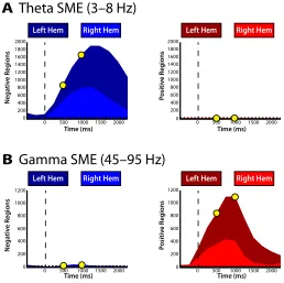
Figure 2.2: Change in theta and gamma power across anatomical location. For two

representa-tive time epochs, 0-1000 ms (early word presentation) and 500-1500 ms (late word presentation), all spherical regions that exhibited a significant (p < 0.001) change in theta (A) and gamma (B) power with successful memory encoding are displayed on a standardized three-dimensional brain. Increases (R> N) and decreases (N<R) in power are shown in red and blue, respectively. The

color scale reflects the percentage of nearby ROI’s exhibiting identical encoding related e↵ects. The

ipant (Figure 2.1C). For each frequency band, we calculated an averaget-statistic for all electrodes in each region by comparing theta and gamma power between successfully and unsuccessfully remembered items during each temporal epoch following word presentation. To assess whether spectral changes are statistically reliable across participants, we used a permutation procedure to map encoding re-lated changes in theta and gamma power to each region (seeMaterials and Methods). We visualized spherical voxels that exhibited a statistically significant (p < 0.001) change in theta and gamma power during successful memory encoding on a stan-dardized three-dimensional brain (Figures 2.2A and 2.2B) during two representa-tive temporal epochs, 0-1000 ms (early word presentation) and 500-1500 ms (late word presentation).

We found a reliable decrease in theta power following the presentation of words that were successfully remembered compared to words that were not remembered across several brain regions (Figure 2.2A). The decreases in theta power were more prominent in posterior temporal regions during early word presentation, but expanded to include frontal and anterior temporal regions during late word presentation. Whereas decreased theta power with successful encoding was by far the most prevalent pattern observed across cortical and medial temporal regions, smaller increases in theta power were observed in the right anterior temporal lobe and in the left anterior frontal lobes immediately after word presentation.

Time (ms) Left Hem Right Hem

Nega tiv e R eg ions Time (ms) Left Hem Right Hem

Positiv e R eg ions 0 200 400 600 800 1000 1200 0 200 400 600 800 1000 1200

0 500 1000 1500 2000 0 500 1000 1500 2000

Time (ms) Left Hem Right Hem

Nega tiv e R eg ions Time (ms) Left Hem Right Hem

Positiv

e R

eg

ions

0 500 1000 1500 2000 0 500 1000 1500 2000

A

Theta SME (3–8 Hz)

B

Gamma SME (45–95 Hz)

0 200 400 600 800 1000 1400 1600 1200 1800 2000 0 200 400 600 800 1200 1400 1600 1000 1800 2000

Figure 2.3: Temporal evolution of changes in theta and gamma power. A: The total number

of regions exhibiting a significant decrease (left panel) or increase (right panel) in both theta (A) and gamma (B) power are displayed across time. Yellow circles represent the early and late word presentation intervals shown in Figure 2.2. Chance level (p=0.001) is represented by the horizontal dashed line. The percentage of the regions in each hemisphere is proportional to the area of the light- and dark-colors, as indicated.

cortices early after item presentation and expanded anteriorly during later inter-vals. In addition, the increases we observe in the gamma range lateralized to the left hemisphere; gamma activations in the right hemisphere were more spatially discrete and co-occurred alongside pockets of decreased gamma power. The left hemispheric bias of gamma activations likely reflects the language comprehension component of our task.

R NR B Lo g P ow er ( μ V 2 )

Theta Power Gamma Power

A B

R NR B

6.0

5.9

5.8 5.7

R NR B

Lo g P ow er ( μ V 2 )

Theta Power Gamma Power

3.2

3.1

R NR B

R NR B

Lo g P ow er ( μ V 2 )

Theta Power Gamma Power

C D

4.3 4.4

R NR B

6.4

R NR B

Lo g P ow er ( μ V 2 )

Theta Power Gamma Power

R NR B

4.4 4.3 4.2 6.8 6.5 6.4 6.6 6.7 6.3 6.2 6.1 6.0 4.1 4.0 3.9 7.2 7.0 6.6 6.8

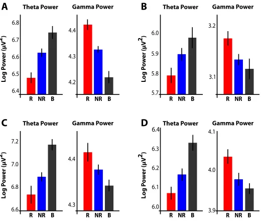
Figure 2.4: Examples of theta and gamma power fluctuations during successful memory forma-tion. For four di↵erent electrodes, raw log-transformed power in the theta (3-8 Hz) and gamma

(45-95 Hz) bands is shown for all subsequently recalled (R; red), subsequently not-recalled (NR; blue), and baseline (B; gray) events. Error bars represent the 95% CI. A: Patient: TJUH-11, Elec-trode location: Left lateral temporal lobe, Brodmann area 20, time epoch: 500-1500 ms; B: Patient: TJUH-19, Electrode location: Right posterior parahippocampal gyrus (depth electrode), time epoch: 250-1250 ms. C: Patient: TJUH-23, Electrode location: Right lateral temporal lobe, Brodmann area 20, time epoch: 500-1500 ms. D: Patient: TJUH-24, Electrode location: Right lateral temporal lobe, Brodmann area 21, time epoch: 500-1500 ms.

change in power during any given time epoch by chance (5.5 regions in each tail of the distribution; dashed line, Figures 2.3A and 2.3B). Figure 2.3 demonstrates that decreases in theta power and increases in gamma power during memory formation far exceeded this expectation and are also tightly-linked to item presentation. The precise timing of these e↵ects suggests that the observed changes in power are driven specifically by item presentation as opposed to more non-specific cognitive processes, such as global shifts in attention.

highlight two important features in our data. First, the simultaneous increase in gamma power and decrease in theta power that accompany memory formation can be detected even at the level of individual electrodes. Second, compared to baseline, theta power tends to decrease and gamma power tends to increase during the presentation of all items, but these changes are amplified during the presentation of successfully encoded items.

Changes in phase-synchrony during encoding

Right Left

A

B

C

Theta

G

amma

0 ms 250 ms 500 ms 750 ms 1000 ms 1250 ms

R > NR

Time

R < NR Sync (Q = 0.10) Sync (Q = 0.05) Power (-Sync)

F F

T T

L L

H H

P P

O O

Power (+Sync)

Figure 2.5: Change in theta and gamma lobe-wise synchrony during memory encoding. A:

limited to small areas of decreased gamma phase-synchrony, which was surpris-ing given the widespread increase in gamma power that occurred simultaneously during memory formation.

Using such ROIs to spatially aggregate phase-synchronous interactions across patients clearly demonstrates that memory encoding modulates oscillatory phase-synchrony, particularly in the theta frequency band. However, a drawback of this approach is that it fails to leverage the principal advantage of ECoG over other modalities such as scalp EEG or MEG: very high spatial resolution. This is particularly important when investigating gamma phase-synchrony, which is correlated on a much finer spatial scale than theta activity (N. K. Logothetis, Kayser, & Oeltermann, 2007).

A

Num

Sig P

airs

200

-500

-600

C

Σ

+1-1 ₊₁

-1

Δ

d

= -1

-1 0

-1 +1

0 0

D

B

0–1000 ms 750–1750 ms

0–1000 ms 750–1750 ms

0

-200

-300 100

-100

-400

Time

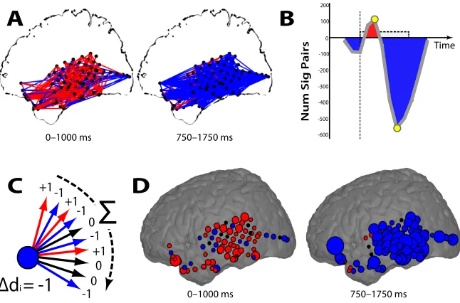
Figure 2.6: Aggregating pair-wise network connections. A: All pairs of electrodes with significant

(p < 0.05) increases (red lines) or decreases (blue lines) in theta synchrony during successful encoding are shown for two di↵erent time epochs for patient TJUH 11. B: For all time epochs,

the di↵erence between the total number of pairs exhibiting a significant increase and decrease in

synchrony is shown. Yellow circles mark the epochs depicted in A. C: The change in degree, dp,

is found by tabulating significant increases or decreases in synchrony for each connection of each electrode. D: The change in degree, dp, for each electrode is shown summarizing the changes in

To more precisely spatially localize changes in phase synchrony during mem-ory encoding, we used a graph theoretic approach. Briefly, we designated every electrode,ep, as a node in a larger network, and calculated the total number of other nodes in the network,eq, that share a statistically significant increase in synchrony with that node minus the total number of other nodes that share a statistically sig-nificant decrease in synchrony during successful memory encoding (Figure 2.6C;

seeMaterials and methods). The resulting change in degree, dp, represents the

ex-tent to which each node in the network increases or decreases its phase-synchrony with the rest of the network during memory encoding. Defining each electrode’s functional connectivity in this manner allows us to localize anatomic areas where memory-related changes in synchrony were most concentrated. Spatially localiz-ing the changes in theta synchrony observed in Figure 2.6A demonstrated that the temporal lobe was marked by increases in theta synchrony during early word pre-sentation, followed by prominent decreases in theta synchrony during late word presentation localized to the left lateral and inferior temporal cortex (Figure 2.6D). Using this approach, we calculated the change in degree for each electrode for each participant and determined if the changes observed in a particular region were statistically significant across all participants. As for our power analysis, we used 5,484 identical spherical voxels uniformly placed across Talairach space to group nearby electrodes for each participant (Figure 2.1D). We used a permutation procedure to assess whether the changes in degree for each region are statistically significant across participants during early (0-1000 ms) and late (500-1500 ms) word presentation (seeMaterials and methods).

Early Word Presentation (0–1000 ms)

Late Word Presentation (500–1500 ms)

A

L R

B

Early Word Presentation (0–1000 ms)

Late Word Presentation (500–1500 ms)

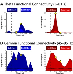
Theta Functional Connectivity (3–8 Hz)

Gamma Functional Connectivity (45–95 Hz)

L R

0%

25% 25%

Significant Regions R > NR

R < NR

25% 0%

Av

ailable R

eg

ions

25% 0%

Av

ailable R

eg

ions

Figure 2.7: Change in theta and gamma degree across anatomic locations. All spherical regions

that exhibited a significant (p < 0.001) change in theta (A) and gamma (B) degree ( dp) during

successful memory encoding are displayed on a standardized three-dimensional brain. Increases and decreases in phase-synchrony are shown in red and blue, respectively. The colorscale and grayscale reflect the percentage of surrounding regions with identical encoding related e↵ects and

with a prominent increase in theta power (see Figure 2.2A), which suggested that power analyses alone were insufficient to isolate these phase-synchronous theta oscillations. After this initial increase, we found that theta synchrony during encoding exhibited reliable decreases localized di↵usely throughout the brain, but which were most concentrated in the left medial temporal lobe. The decrease in theta synchrony overlapped in time and space with regions in which theta power also decreased. These results extend the ROI approach to demonstrate that the left pre-frontal cortex, more than any other region, is the major hub of the theta synchronous verbal episodic memory encoding network.

When we examined changes in gamma synchrony, on the other hand, we found distinct regions of gamma synchrony during memory encoding (Figure 2.7B). This result highlights the utility investigating spatially precise synchronous interactions. In particular, we found that successful memory encoding involved either no change or an overall decrease in gamma synchrony in the left hemisphere. This result was surprising given the highly reliable increases in gamma power that occurred simultaneously in the same region (see Figure 2.2B). In addition, we found increased gamma synchrony that localized to the right hemisphere in the frontal-temporal (peri-sylvian) areas of the brain.

consis-Time (ms) Left Hem Right Hem

Nega tiv e R eg ions Time (ms) Left Hem Right Hem

Positiv

e R

eg

ions

0 500 1000 1500 2000 0 500 1000 1500 2000

A

Theta Functional Connectivity (3–8 Hz)

B

Gamma Functional Connectivity (45–95 Hz)

Time (ms) Left Hem Right Hem

Nega tiv e R eg ions Time (ms) Left Hem Right Hem

Positiv

e R

eg

ions

0 500 1000 1500 2000 0 500 1000 1500 2000

0 50 100 150 5 10 20 25 30 35 45 0 15 40 5 10 20 25 30 35 45 0 15 40 0 50 100 150

Figure 2.8: Temporal evolution of changes in theta and gamma degree. The total number of

regions exhibiting a significant decrease (left panel) or increase (right panel) in both theta (A) and gamma (B) connectivity ( dp) are displayed across time. Yellow circles represent the early and

tent hemispheric lateralization of gamma phase-synchrony such that increases in synchrony were prominent in the right hemisphere and decreases in phase-synchrony were prominent in the left hemisphere (Figure 2.8B). Although gamma synchrony was reliably modulated by memory formation, the temporal envelope defining these changes was not as well defined.

2.5 Discussion

of the electrophysiological profile accompanying human verbal episodic memory encoding, our results help clarify the role of rhythmic neural activity in the memory system.

Theta Phase Synchrony

phase-synchrony during later temporal epochs of successful memory encoding, localized to the left hemisphere and accompanied by broad anteriorly-spreading decreases in theta power. The degree to which memory formation involves this decrease in theta power represents perhaps the most striking finding in our data, and is consistent with previous EEG and MEG findings (Sederberg et al., 2007; Guderian et al., 2009, see Figure 2.2). Such task-related decreases in low fre-quency power have been traditionally classified as event related desynchroniza-tions (Crone, Miglioretti, Gordon, & Lesser, 1998; Pfurtscheller & Lopes Da Silva, 1999) under the assumption that they reflect a decrease in synchronized local neural activity (Singer, 1993). Here, we show that the decrease in theta power during mem-ory formation is also accompanied by late decreases in long-range theta synchrony. This asynchronous activity may simply reflect a passive deactivation following theta synchronization, but another possibility is that the asynchronous activity it-self may play a role in memory formation. Indeed, decreases in low-frequency power and synchrony correlate with the BOLD signal (Kilner, Henson, & Friston, 2005; Niessing et al., 2005) and have been shown to co-vary with transitions to ac-tive cortical states (Harris & Thiele, 2011; Poulet, Fernandez, Crochet, & Petersen, 2012). Whether memory formation represents a similar transition to a more active cortical state is unclear, but the asynchronous activity we detect here suggests this intriguing possibility.

during successful encoding (Figures 2.5-2.8) helps to explain this ambiguity by suggesting that theta power reflects two dissociable processes: power decreases vs. synchronous oscillations. Each of these two competing e↵ects may be detected to a lesser or greater degree depending on the particular experimental conditions or post-processing steps implemented. By precisely categorizing the subtle yet re-liable nuances of theta activity during memory formation, it is possible to interpret apparently diverging results within a common electrophysiological framework.

Gamma phase synchrony

We observed increases in gamma synchrony during successful memory encoding in the peri-sylvian areas of the right hemisphere. This result suggests that gamma activity in this region represents true narrow-band oscillations, which is generally consistent with predictions regarding the role of gamma synchrony in memory formation (Jensen et al., 2007; Jutras & Bu↵alo, 2010; Fell & Axmacher, 2011). The location of this synchronous gamma network (R. peri-sylvian) may seem at odds with the previous work reporting increased synchrony between rhinal cor-tex and hippocampus during memory formation (Fell et al., 2001), however two important features of our analyses may explain this discrepancy. First, the ROI ap-proach averaged electrode interactions over spatially course regions and, second, the graph-theoretical approach was designed to detect hubs of network activity. Thus, if gamma synchronous oscillations were limited to a single electrode pair amidst all possible pairs, as the Fell et al. study indicates, they would not be opti-mally detected in our analyses that specifically avoided making prior assumptions regarding anatomical localization.

is observed across a wide-range of brain areas during memory formation, repre-sents phase-synchronous oscillations in the general sense. Using this approach, we found that the most reliable increases in gamma power during memory formation were localized to the left hemisphere and were accompanied by less synchrony than expected by chance during memory formation. It is unlikely that our fail-ure to observe increases in gamma synchrony in the left hemisphere reflects a methodological shortcoming. Although our temporal windows of 1000 ms are large relative to the length of a gamma cycle, we calculated phase-synchrony using wavelets with a finer temporal resolution (2 temporal envelope of the 95 Hz and 45 Hz wavelets: 33.5 ms and 70.7 ms), which was sufficient to detect transient increases in gamma synchrony in other brain regions. Instead, the decreases in high frequency synchrony we observe here likely reflect asynchronous noise fluc-tuations related to multi-unit neural activity (Ray & Maunsell, 2011; Manning et al., 2009; Miller, Zanos, et al., 2009) or transient ”bottom-up” responses (Ossand´on et al., 2012), and suggest that increases in gamma power in these regions do not represent temporally binding synchronous oscillations (Jutras & Bu↵alo, 2010; Fell & Axmacher, 2011). Although the origins of high-frequency activations are still un-clear (Crone, Korzeniewska, & Franaszczuk, 2011; Buzs´aki & Wang, 2012; Lachaux, Axmacher, Mormann, Halgren, & Crone, 2012), our results suggest that the degree of synchrony within the gamma band can dissociate between gamma oscillations on the one hand and broadband activations on the other (Jia, Smith, & Kohn, 2011).

Conclusion and future directions

shown to interact with spectral responses and coherence measures (Wang, Chen, & Ding, 2008; Wang & Ding, 2011). Whereas it is possible to factor out such evoked responses, doing so requires special models and analytical techniques (Truccolo, Ding, Knuth, Nakamura, & Bressler, 2002; Xu et al., 2009). Future studies would benefit from incorporating such models to further dissociate induced synchronous activity from asynchronous evoked sources.

Chapter 3

Human intracranial high-frequency

activity maps episodic memory

formation in space and time

John F. Burke, Nicole, M. Long, Kareem A. Zaghloul, Ashwini D. Sharan, Michael R. Sperling, and Michael J. Kahana (2013). NeuroImage, In press, DOI: 10.1016/j.neuroimage.2013.06.067.

3.1 Abstract

as well as the medial temporal lobe and late increases in HFA that involve the left inferior frontal gyrus, left posterior parietal cortex and left ventrolateral temporal cortex. We speculate that these activations reflect higher-order visual processing and top-down modulation of attention/semantic information, respectively.

3.2 Introduction

Among those experiences that enter the focus of our attention, some are encoded in a manner that can easily support subsequent recollection while others are not. This variability in goodness of memory encoding has been the subject of considerable psychological research over the last century (Kahana, 2012), yet only in the last decade or so have we begun to uncover its physiological basis. In the laboratory, one can investigate the neural basis of goodness of encoding by recording brain signals from participants while they engage in a learning task and then correlating specific features in the signal with subsequent memory performance (Paller & Wagner, 2002).

To investigate the spatiotemporal properties of this memory encoding network, it is necessary to use a brain signal with millisecond temporal resolution, such as intracranially recorded high-frequency activity (HFA). HFA refers to fast fluctua-tions in neuro-electrophysiological recordings that manifest as increases in spectral power at frequencies above 60-70 Hz. The neural mechanism that gives rise to such fast activity is a topic of on-going research: HFA has been linked to asyn-chronous “shot-noise” related to increased multi-unit activity (Milstein, Mormann, Fried, & Koch, 2009; Manning et al., 2009; Miller, Sorensen, et al., 2009; Ray & Maunsell, 2011), the superposition of multiple high-frequency oscillations (Crone et al., 2011; Gaona et al., 2011), as well as a combination of these two processes (Sche↵er-Teixeira, Belchior, Le˜ao, Ribeiro, & Tort, 2013). Despite its unclear neural origin, however, an increasing number of studies have leveraged HFA as a marker of underlying neural activation (Crone et al., 2011; Lachaux et al., 2012), similar to the blood-oxygen-level-dependent (BOLD) signal. Indeed, HFA has been directly correlated with BOLD activity (Mukamel et al., 2005; Conner, Ellmore, Pieters, DiS-ano, & Tandon, 2011), further suggesting that HFA represents a marker of general neural activation.

more general metric of neural activation, the information conveyed by this signal should be reflected in the exact time and spatial location in which it is active. By collecting data from a very large number of patients (ninety-eight), we were able to overcome the limited spatial sampling of human intracranial electrophysiology and use HFA to map memory encoding in both space and time. This approach revealed a dynamic spatiotemporal activation of functional networks that mediate encoding, as described in this report.

3.3 Methods

3.3.1 Participants

Participants with medication-resistant epilepsy underwent a surgical procedure in which grid, strip, and depth electrodes were implanted so as to localize epilepto-genic regions. Data were collected over a 14 year period as part of a multi-center collaboration with neurology and neurosurgery departments across the country. Our research protocol was approved by the institutional review board at each hos-pital and informed consent was obtained from the participants and their guardians. Our final participant pool consisted of 98 patients (left-language dominant patients; see Table 2.1).

3.3.2 Free Recall Task