Essays in Asset Pricing and Tail Risk

(1)

University of Pennsylvania

ScholarlyCommons

Publicly Accessible Penn Dissertations

1-1-2015

Essays in Asset Pricing and Tail Risk

Sang Byung Seo

University of Pennsylvania, sangseo@wharton.upenn.edu

Follow this and additional works at:

http://repository.upenn.edu/edissertations

Part of the

Finance and Financial Management Commons

Recommended Citation

(2)

Essays in Asset Pricing and Tail Risk

Abstract

The first chapter "Option Prices in a Model with Stochastic Disaster Risk," co-authored with Jessica Wachter, studies the consistency between the rare disaster mechanism and options data. In contrast to past work based on an iid setup, we find that a model with stochastic disaster risk can explain average implied volatilities well, despite being calibrated to consumption and aggregate market data alone. Furthermore, we extend the stochastic disaster risk model to a two-factor model and show that it can match variation in the level and slope of implied volatilities, as well as the average implied volatility curves.

The second chapter "Do Rare Events Explain CDX Tranche Spreads?," also co-authored with Jessica Wachter, investigates the rare disaster mechanism based on the data on the CDX index and its tranches. Senior tranches are essentially deep out-of-the-money options because they do not incur any losses until a large number of investment-grade firms default. Using the two-factor stochastic disaster model, we jointly explain the spreads on each CDX tranche, as well as prices on put options and the aggregate market. This paper demonstrates the importance of beliefs about rare disasters and shows a basic consistency in these beliefs across different asset markets.

In the third chapter, "Correlated Defaults and Economic Catastrophes: Linking the CDS Market and Asset Returns," I consider economic catastrophes as massive correlated defaults and construct a catastrophic tail risk measure from joint default probabilities based on my model as well as information contained in the CDS data. Using the rich information contained in this measure, I find that investors put more weight on future extreme events even after the stock market showed signs of recovery from the recent financial crisis. Furthermore, I show that high catastrophic tail risk robustly predicts high future excess returns for various assets, including stocks, government bonds, and corporate bonds. This risk is negatively priced, generating substantial dispersion in the cross section of stock returns. These results consistently indicate that seemingly impossible economic catastrophes are considered as an important risk source when trading assets.

Degree Type

Dissertation

Degree Name

Doctor of Philosophy (PhD)

Graduate Group

Finance

First Advisor

Jessica A. Wachter

Keywords

(3)

Subject Categories

(4)

ESSAYS IN ASSET PRICING AND TAIL RISK

Sang Byung Seo

A DISSERTATION

in

Finance

For the Graduate Group in Managerial Science and Applied Economics

Presented to the Faculties of the University of Pennsylvania

in

Partial Fulfillment of the Requirements for the

Degree of Doctor of Philosophy

2015

Supervisor of Dissertation

Signature

Jessica A. Wachter

Richard B. Worley Professor of Financial Management, Professor of Finance

Graduate Group Chairperson

Signature

Eric T. Bradlow

K.P. Chao Professor of Marketing, Statistics, and Education

Dissertation Committee

(5)

ACKNOWLEDGEMENT

First and foremost, I am deeply grateful to my advisors Nikolai Roussanov, Jessica Wachter,

and Amir Yaron for their invaluable guidance.

I would also like to thank my friends and classmates who made my time at Wharton more

enjoyable: Ian Appel, Christine Dobridge, Michael Lee, Gil Segal, and Colin Ward. I would

like to especially thank Mete Kilic for his amazing help and feedback.

(6)

ABSTRACT

ESSAYS IN ASSET PRICING AND TAIL RISK

Sang Byung Seo

Jessica A. Wachter

The first chapter “Option Prices in a Model with Stochastic Disaster Risk,” co-authored

with Jessica Wachter, studies the consistency between the rare disaster mechanism and

options data. In contrast to past work based on an iid setup, we find that a model with

stochastic disaster risk can explain average implied volatilities well, despite being calibrated

to consumption and aggregate market data alone. Furthermore, we extend the stochastic

disaster risk model to a two-factor model and show that it can match variation in the level

and slope of implied volatilities, as well as the average implied volatility curves.

The second chapter “Do Rare Events Explain CDX Tranche Spreads?,” also co-authored

with Jessica Wachter, investigates the rare disaster mechanism based on the data on the

CDX index and its tranches. Senior tranches are essentially deep out-of-the-money options

because they do not incur any losses until a large number of investment-grade firms default.

Using the two-factor stochastic disaster model, we jointly explain the spreads on each CDX

tranche, as well as prices on put options and the aggregate market. This paper demonstrates

the importance of beliefs about rare disasters and shows a basic consistency in these beliefs

across different asset markets.

In the third chapter, “Correlated Defaults and Economic Catastrophes: Linking the CDS

Market and Asset Returns,” I consider economic catastrophes as massive correlated

de-faults and construct a catastrophic tail risk measure from joint default probabilities based

on my model as well as information contained in the CDS data. Using the rich

(7)

Furthermore, I show that high catastrophic tail risk robustly predicts high future excess

returns for various assets, including stocks, government bonds, and corporate bonds. This

risk is negatively priced, generating substantial dispersion in the cross section of stock

re-turns. These results consistently indicate that seemingly impossible economic catastrophes

(8)

TABLE OF CONTENTS

ACKNOWLEDGEMENT . . . ii

ABSTRACT . . . iii

LIST OF TABLES . . . vii

LIST OF ILLUSTRATIONS . . . ix

CHAPTER 1 : Option Prices in a Model with Stochastic Disaster Risk . . . 1

1.1 Introduction . . . 1

1.2 Option prices in a single-factor stochastic disaster risk model . . . 5

1.3 Average implied volatilities in the model and in the data . . . 11

1.4 Option prices in a multi-factor stochastic disaster risk model . . . 18

1.5 Fitting the multifactor model to the data . . . 21

1.6 Conclusion . . . 27

CHAPTER 2 : Do Rare Events Explain CDX Tranche Spreads? . . . 47

2.2 Model . . . 48

2.3 Evaluating the model . . . 56

CHAPTER 3 : Correlated Defaults and Economic Catastrophes: Linking the CDS Market and Asset Returns . . . 75

3.2 Model of correlated defaults . . . 80

3.3 CAT measure - Implied catastrophic tail risk . . . 90

(9)

3.5 Model estimation procedure . . . 96

3.6 Interpretation of estimation results . . . 103

3.7 Implications for catastrophic tail risk . . . 107

3.8 Implications for asset returns . . . 112

APPENDIX . . . 143

(10)

LIST OF TABLES

TABLE 1.1 : Parameter values . . . 43

TABLE 1.2 : Parameter values for the two-factor SDR model . . . 44

TABLE 1.3 : Moments for the government bill rate and the market return for the two-factor SDR model . . . 45

TABLE 1.4 : Moments of state variables in the two-factor SDR model . . . 46

TABLE 2.1 : Parameter values for the model . . . 73

TABLE 2.2 : Parameter values for an individual firm . . . 74

TABLE 3.1 : Correlation matrix of CAT measures with different extremities . . . 134

TABLE 3.2 : Correlation matrix of CAT measures with same extremities but dif-ferent horizons . . . 134

TABLE 3.3 : Correlation matrix of CAT measures and other classic stock return predictors . . . 135

TABLE 3.4 : Persistence of CAT measures and other classic stock return predictors135 TABLE 3.5 : Correlation matrix of individual CAT measures and tail risk measures135 TABLE 3.6 : Univariate predictive regressions of stock returns . . . 136

TABLE 3.7 : Multivariate predictive regressions of 2-year horizon stock returns . 137 TABLE 3.8 : VAR-impliedR2 . . . 138

TABLE 3.9 : Univariate predictive regressions of government bond returns . . . 139

TABLE 3.10 :Multivariate predictive regressions of 5-year maturity government bond returns . . . 140

TABLE 3.11 :Predictive regressions of corporate bond returns . . . 141

(11)

LIST OF ILLUSTRATIONS

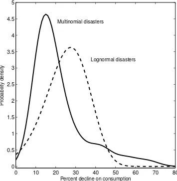
FIGURE 1.1 : Probability density functions for consumption declines . . . 30

FIGURE 1.2 : Average implied volatilities in the SDR and CDR models . . . 31

FIGURE 1.3 : Comparative statics for the CDR model . . . 32

FIGURE 1.4 : Evaluating the role of recursive utility . . . 33

FIGURE 1.5 : Implied volatilities for given values of the disaster probability . . 34

FIGURE 1.6 : 1-month implied volatility time series . . . 35

FIGURE 1.7 : Mean and volatility of implied volatilities in simulated data . . . . 36

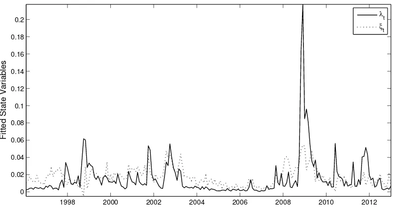
FIGURE 1.8 : Fitted values of state variables . . . 37

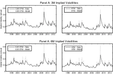
FIGURE 1.9 : 3- and 6-month implied volatility time series . . . 38

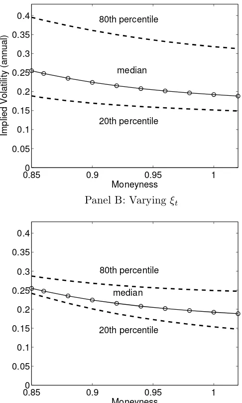
FIGURE 1.10 :Implied volatilities as functions of the state in the two-factor SDR model . . . 39

FIGURE 1.11 :Average implied volatilities from the time series of state variables 40 FIGURE 1.12 :The price-dividend ratio in the data and in the model . . . 41

FIGURE A.1 : Exact versus approximate solution . . . 42

FIGURE A.1 : Average implied volatilities . . . 65

FIGURE A.2 : Term structure of tranche spreads . . . 66

FIGURE A.3 : Average CDX tranche spreads (5Y) . . . 67

FIGURE A.6 : CDX index and CDX tranches time series (5Y) . . . 70

(12)

FIGURE A.3 : Implied beliefs of investors . . . 125

FIGURE A.4 : Time series of the average firm’s CDS curves: level and slope . . . 126

FIGURE A.5 : CDS term structure of the average firm in the model and data . . 127

FIGURE A.6 : Individual firm dynamics: two examples . . . 128

FIGURE A.7 : CAT surfaces in the pre-crisis, crisis, and post-crisis period . . . . 129

FIGURE A.8 : Time series of CAT surfaces . . . 130

FIGURE A.9 : 10-year catastrophic tail distribution in the pre-crisis, crisis, and

post-crisis period . . . 131

FIGURE A.10 :Term structure of the CAT measure in the pre-crisis, crisis, and

post-crisis period . . . 132

(13)

CHAPTER 1 : Option Prices in a Model with Stochastic Disaster Risk

(with Jessica A. Wachter)

1.1. Introduction

Century-long evidence indicates that the equity premium, namely the, expected return

from holding equities over short-term debt, is economically significant. Ever since Mehra

and Prescott (1985) noted the puzzling size of this premium relative to what a standard

model would predict, the source of this premium has been a subject of debate. One place

to look for such a source is in options data. By holding equity and a put option, an investor

can, at least in theory, eliminate the downside risk in equities. For this reason, it is appealing

to explain both options data and standard equity returns together with a single model.

Such an approach is arguably of particular importance for a class of macro-finance models

that explain the equity premium through the mechanism of consumption disasters (e.g. Rietz

(1988), Barro (2006) and Weitzman (2007)). In these models, consumption growth rates

and thus equity returns are subject to shocks that are rare and large. Options (assuming

away, for the moment, the potentially important question of counterparty risk), offer a way

to insure against the risk of these events. Thus it is of interest to know whether these

models have the potential to explain option prices as well as equity prices.

Thus, option prices convey information about the price investors require to insure against

losses, and therefore indirectly about the source of the equity premium. Indeed, prior

literature uses option prices to infer information about the premium attached to crash risk

(e.g. Pan (2002)); recent work connects this risk to the equity premium as a whole (Bollerslev

and Todorov (2011b) and Santa-Clara and Yan (2010)). Despite the clear parallel to the

literature on consumption disasters and the equity premium, the literatures have advanced

(14)

also a difference in terminology (which reflects a difference in the philosophy). In the options

literature, the focus is on sudden negative changes in prices, called crashes; connections to

economic fundamentals are not modeled. In the macro-finance literature, the focus is on

disasters as reflected in economic fundamentals like consumption or GDP, rather than the

behavior of stock prices. However, in both literatures, risk premia are specifically attributed

to events whose size and probability of occurrence renders a normal distribution essentially

impossible.

Motivated by the parallels between these very different literatures, Backus, Chernov, and

Martin (2011) study option prices in a consumption disaster model similar to that of Rietz

(1988) and Barro (2006). They find, strikingly, that options prices implied by the

con-sumption disaster model are far from their data counterparts. In particular, the implied

volatilities resulting from a calibration to macroeconomic consumption data are lower than

in the data, and are far more downward sloping as a function of the strike price. Thus

options data appear to be inconsistent with consumption disasters as an explanation of the

equity premium puzzle.

Like Barro (2006) and Rietz (1988), Backus, Chernov, and Martin (2011) assume that the

probability of a disaster occurring is constant. Such a model can explain the equity premium,

but cannot account for other features of equity markets, such as the volatility. Recent rare

events models therefore introduce dynamics that can account for equity volatility (Gabaix

(2012), Gourio (2012), Wachter (2013)). We derive option prices in a model based on that

of Wachter (2013), and in a significant generalization of this model that allows for variation

in the risk of disaster at different time scales. We show that allowing for a stochastic

probability of disaster has dramatic effects on implied volatilities. Namely, rather than

being much lower than in the data, the implied volatilities are at about the same level. The

slope of the implied volatility curve, rather than being far too great, also matches that of

the data. We then apply the model to understanding other features of option prices in the

(15)

that the model can account for these features of the data as well. In other words, a model

calibrated to international consumption data on disasters can explain option prices after

all.

We use the fact that our model generalizes the previous literature to better understand

the difference in results. Because of time-variation in the disaster probability, the model

endogenously produces the stock price changes that occur during normal times and that

are reflected in option prices. These changes are absent in iid rare event models, because,

during normal times, the volatility of stock returns is equal to the (low) volatility of dividend

growth. Moreover, by assuming recursive utility, the model implies a premium for assets

that covary negatively with volatility. This makes implied volatilities higher than what they

would be otherwise.

Our findings relate to those of Gabaix (2012), who also reports average implied volatilities in

a model with rare events.1 Our model is conceptually different in that we assume recursive

utility and time-variation in the probability of a disaster. Gabaix assumes a

linearity-generating process (Gabaix (2008)) with a power utility investor. In his calibration, the

sensitivity of dividends to changes in consumption is varying; however, the probability

of a disaster is not. There are several important implications of our choice of approach.

First, the tractability of our framework implies that we can use the same model for pricing

options as we do for equities. Moreover, our model nests the simpler one with constant

risk of disaster, allowing us to uncover the reason for the large difference in option prices

between the models. We also show that the assumption of recursive utility is important for

the accounting for the average implied volatility curve. Finally, we go beyond the average

implied volatility curve for 3-month options, considering the time series in the level and

slope of the implied volatility curve across different maturities. These considerations lead

us naturally to a two-factor model for the disaster probability.

(16)

Other recent work explores implications for option pricing in dynamic endowment economies.

Benzoni, Collin-Dufresne, and Goldstein (2011) derive options prices in a Bansal and Yaron

(2004) economy with jumps to the mean and volatility of dividends and consumption. The

jump probability can take on two states which are not observable to the agent. Their focus

is on the learning dynamics of the states, and the change in option prices before and after

the 1987 crash, rather than on matching the shape of the implied volatility curve. Du

(2011) examines options prices in a model with external habit formation preferences as in

Campbell and Cochrane (1999) in which the endowment is subject to rare disasters that

occur with a constant probability. His results illustrate the difficulty of matching implied

volatilities assuming either only external habit formation, or a constant probability of a

disaster. Also related is the work of Drechsler and Yaron (2011), who focus on the volatility

premium and its predictive properties. Our paper differs from these in that we succeed in

fitting both the time series and cross-section of implied volatilities, as well as reconciling

the macro-finance evidence on rare disasters with option prices.

A related strand of research on endowment economies focuses on uncertainty aversion or

exogenous changes in confidence. Drechsler (2012) builds on the work of Bansal and Yaron

(2004), but incorporates dynamic uncertainty aversion. He argues that uncertainty

aver-sion is important for matching implied volatilities. Shaliastovich (2009) shows that jumps

in confidence can explain option prices when investors are biased toward recency. These

papers build on earlier work by Bates (2008) and Liu, Pan, and Wang (2005), who conclude

that it is necessary to introduce a separate aversion to crashes to simultaneously account

for data on options and on equities. Buraschi and Jiltsov (2006) explain the pattern in

implied volatilities using heterogenous beliefs. Unlike these papers, we assume a rational

expectations investor with standard (recursive) preferences. The ability of the model to

explain implied volatilities arises from time-variation in the probability of a disaster rather

than a premium associated with uncertainty.

(17)

option prices, and risk premia. Brunnermeier, Nagel, and Pedersen (2008) links option

prices to the risk of currency crashes, Kelly, Lustig, and Van Nieuwerburgh (2012) use

options to infer a premium for too-big-to-fail financial institutions, Gao and Song (2013)

price crash risk in the cross-section using options, and Kelly, Pastor, and Veronesi (2014)

demonstrate a link between options and political risk. The focus of these papers is empirical.

Our model provides a model that can help in interpreting these results.

The remainder of this paper is organized as follows. Section 1.2 discusses a single-factor

model for stochastic disaster risk (SDR). This model turns out to be sufficient to explain why

stochastic disaster risk can explain the level and slope of implied volatilities, as explained

in Section 1.3, which also compares the implications of the single-factor SDR model to

the implications of a constant disaster risk (CDR) model. As we explain in Section 1.4,

however, the single-factor model cannot explain many interesting features of options data.

In this section, we explore a multi-factor extension, which we fit to the data in Section 1.5.

We show that the multi-factor model can explain the time-series variation in the implied

volatility slope. Section 1.6 concludes.

1.2. Option prices in a single-factor stochastic disaster risk model

1.2.1. Assumptions

In this section we describe a model with stochastic disaster risk (SDR). We assume an

endowment economy with complete markets and an infinitely-lived representative agent.

Aggregate consumption (the endowment) solves the following stochastic differential equation

dCt=µCt−dt+σC_t−dB_t+ (eZt−1)C_t−dN_t, (1.1)

where Bt is a standard Brownian motion and Nt is a Poisson process with time-varying

(18)

where Bλ,t is also a standard Brownian motion, and Bt, Bλ,t and Nt are assumed to be

independent. For the range of parameter values we consider, λt is small and can therefore

be interpreted to be (approximately) the probability of a jump. We thus will use the

terminology probability and intensity interchangeably, while keeping in mind the that the

relation is an approximate one.

The size of a jump, provided that a jump occurs, is determined byZt. We assume Zt is a

random variable whose time-invariant distributionν is independent ofNt,Bt andBλ,t. We

will use the notationEν to denote expectations of functions ofZttaken with respect to the

ν-distribution. The tsubscript on Zt will be omitted when not essential for clarity.

We will assume a recursive generalization of power utility that allows for preferences over

the timing of the resolution of uncertainty. Our formulation comes from Duffie and Epstein

(1992), and we consider a special case in which the parameter that is often interpreted as the

elasticity of intertemporal substitution (EIS) is equal to 1. That is, we define continuation

utilityVtfor the representative agent using the following recursion:

Vt=Et

Z ∞

t

f(Cs, Vs)ds, (1.3)

where

f(C, V) =β(1−γ)V

logC− 1

1−γ log((1−γ)V)

. (1.4)

The parameterβ is the rate of time preference. We follow common practice in interpreting

γ as relative risk aversion. This utility function is equivalent to the continuous-time limit

(and the limit as the EIS approaches one) of the utility function defined by Epstein and Zin

(19)

1.2.2. Solving for asset prices

We will solve for asset prices using the state-price density, πt.2 Duffie and Skiadas (1994)

characterize the state-price density as

πt= exp

Z t

0

∂

∂Vf(Cs, Vs)ds

∂

∂Cf(Ct, Vt). (1.5)

There is an equilibrium relation between utility Vt, consumptionCt and the disaster

prob-ability λt. Namely,

Vt=

C_t1−γ

1−γe

a+bλt_,

whereaand b are constants given by

a = 1−γ

β

µ−1

2γσ

2

+bκλ¯

β (1.6)

b = κ+β

σ_λ2 −

s

κ+β σ_λ2

2

−2Eν

e(1−γ)Z₋₁

σ_λ2 . (1.7)

It follows that

πt= exp

ηt−βb

Z t

0

λsds

βC_t−γea+bλt_, _(1.8)

whereη =−β(a+ 1). Details are provided in Appendix A1.2.1.

Following Backus, Chernov, and Martin (2011), we assume a simple relation between

div-idends and consumption: Dt=Ctφ, for leverage parameter φ.3 Let F(Dt, λt) be the value

of the aggregate market (it will be apparent in what follows thatF is a function ofDt and

λt). It follows from no-arbitrage that

F(Dt, λt) =Et

Z ∞

t

πs

πt

Dsds

.

2_{Other work on solving for equilibria in continuous-time models with recursive utility includes}

(20)

The stock price can be written explicitly as

F(Dt, λt) =DtG(λt), (1.9)

where the price-dividend ratio Gis given by

G(λt) =

Z ∞

0

exp{aφ(τ) +bφ(τ)λt}

for functions aφ(τ) and bφ(τ) given by:

aφ(τ) =

µD−µ−β+γσ2(1−φ)−

κ¯λ

σ_λ2(ζφ+bσ

2

λ−κ)

τ

−2κλ¯ σ2

λ

log (ζφ+bσ

2

λ−κ) e

−ζφτ₋₁_{+ 2}_ζ

φ

2ζφ

!

bφ(τ) =

2Eν

e(1−γ)Z−e(φ−γ)Z

1−e−ζφτ

(ζφ+bσ_λ2−κ) 1−e−ζφτ

−2ζφ

,

where

ζφ=

q

bσ2_λ−κ2+ 2Eν

e(1−γ)Z₋_e(φ−γ)Z

σ2_λ

(see Wachter (2013)). We will often use the abbreviationFt=F(Dt, λt) to denote the value

of the stock market index at timet.

1.2.3. Solving for implied volatilities

Let P(Ft, λt, τ;K) denote the time-t price of a European put option on the stock market

index with strike priceK and expirationt+τ. For simplicity, we will abbreviate the formula

for the price of the dividend claim as Ft=F(Dt, λt). Because the payoff on this option at

expiration is (K−Ft+τ)+, it follows from the absence of arbitrage that

P(Ft, λt, T −t;K) =Et

πT

πt

(K−FT)+

(21)

LetKn=K/Ft, the normalized strike price (or “moneyness”), and define

Pn(λt, T −t;Kn) =Et

"

πT

πt

Kn−FT Ft

+#

. (1.10)

We will establish below thatPnis indeed a function ofλt, time to expiration and moneyness

alone Clearly P_tn = Pt/Ft. Because our ultimate interest is in implied volatilities, and

because, in the formula of Black and Scholes (1973), normalized option prices are functions

of the normalized strike price (and the volatility, interest rate and time to maturity), it

suffices to calculate P_tn.4

Returning to the formula for Pn

t , we note that, from (1.9), it follows that

FT

Ft

= DT

Dt

G(λT)

G(λt)

. (1.11)

Moreover, it follows from (1.8) that

πT πt = CT Ct −γ exp Z T t

(η−βbλs)ds+b(λT −λt)

. (1.12)

At timet,λtis sufficient to determine the distributions of consumption and dividend growth

betweentandT, as well as the distribution ofλsfors=t, . . . , T. It follows that normalized

put prices (and therefore implied volatilities) are a function of λt, the time to expiration,

and moneyness.

4

Given stock priceF, strike priceK, time to maturity T−t, interest rater, and dividend yieldy, the Black-Scholes put price is defined as

BSP(F, K, T−t, r, y, σ) =e−r(T−t)KN(−d2)−e−y(T−t)F N(−d1)

where

d1=

log(F/K) + r−y+σ2/2 (T−t)

σ√T−t and d2=d1−σ

√

T−t

Given the put prices calculated from the transform analysis, inversion of this Black-Scholes formula gives us implied volatilities. Specifically, the implied volatilityσimpt =σ

imp

(λt, T−t;Kn) solves

Ptn(λt, T −t;Kn) = BSP

1, Kn, T−t, rbt,1/G(λt), σimpt

(22)

Appendix A1.2.5 describes the calculation of (1.10). We first approximate the price-dividend

ratio G(λt) by a log-linear function of λt, As the Appendix describes, this approximation

is highly accurate. We can then apply the transform analysis of Duffie, Pan, and Singleton

(2000) to calculate put prices.

The implied volatility curve in the data represents an average of implied volatilities at

differ-ent points in time. We follow the same procedure in the model, calculating an unconditional

average implied volatility curve. To do so, we first solve for the implied volatility as a

func-tion of λt. We numerically integrate this function over the stationary distribution of λt.

This stationary distribution is Gamma with shape parameter 2κλ/σ¯ _λ2 and scale parameter

σ_λ2/(2κ) (Cox, Ingersoll, and Ross (1985)).

1.2.4. The constant disaster risk model

Taking limits in the above model as σλ approaches zero implies a model with a constant

probability of disaster (Appendix A1.2.2 shows that this limit is indeed well-defined and is

what would be computed if one were to solve the constant disaster risk model from first

principles). We use this model to evaluate the role that stochastic disaster risk plays in the

model’s ability to match the implied volatility data. We refer to this model in what follows

as the CDR (constant disaster risk) model, to distinguish it from the more general SDR

model.

The CDR model is particularly useful in reconciling our results with those of Backus,

Cher-nov, and Martin (2011). Backus et al. solve a model with a constant probability of a

jump in consumption, calibrated in a manner similar to Barro (2006). They call this the

consumption-based model, to distinguish it from the reduced-form options-based model

which is calibrated to fit options data. While Backus et al. assume power utility, their

model can be rewritten as one with recursive utility with an EIS of one. The reason is that

the endowment process is iid. In this special case, the EIS and the discount rate are not

(23)

factor, and therefore identical asset prices to a recursive utility model with arbitrary EIS

as long as one can adjust the discount rate (Appendix A1.2.3).5

1.3. Average implied volatilities in the model and in the data

In this section we compare implied volatilities in the two versions of the model we have

discussed with implied volatilities in the data. For now, we focus on three-month options.

Table 1.1 shows the parameter values for the SDR and the benchmark CDR model. The

parameters in the SDR model are identical to those of Wachter (2013), and thus do not

make use of options data. The parameters for the benchmark CDR model are as in the

consumption-based model of Backus, Chernov, and Martin (2011). That is, we consider

a calibration that is isomorphic to that of Backus, Chernov, and Martin (2011) in which

the EIS is equal to 1. Assuming a riskfree rate of 2% (as in Backus et al.), we calculate

a discount rate of 0.0189 . We could also use the same parameters as in the SDR model

except with σλ = 0; the results are very similar.

The two calibrations differ in their relative risk aversion, in the volatility of normal-times

consumption growth, in leverage, in the probability of a disaster, and of course in whether

the probability is time-varying. The net effect of some of these differences turns out to

be less important than what one may think: for example, higher risk aversion and lower

disaster probability roughly offset each other. We explore the implications of leverage and

volatility in what follows.

The two models also assume different disaster distributions. For the SDR model, the

dis-aster distribution is multinomial, and taken from Barro and Ursua (2008) based on actual

consumption declines. The benchmark CDR model assumes that consumption declines are

5

(24)

log-normal. For comparison, we plot the smoothed density for the SDR model along with

the density of the consumption-based model in Figure 1.1. Compared with the lognormal

model, the SDR model has more mass over small declines in the 10–20% region, and more

mass over large declines in the 50-70% region.6

Figure 1.2 shows the resulting implied volatilities as a function of moneyness, as well as

implied volatilities in the data. Confirming previous results, we find that the CDR model

leads to implied volatilities that are dramatically different from those in the data. First,

the implied volatilities are too low, even though the model was calibrated to match the

volatility of equity returns. Second, they exhibit a strong downward slope as a function of

the strike price. While there is a downward slope in the data, it is not nearly as large. As a

result, implied volatilities for at-the-money (ATM) options in the CDR model are less than

10%, far below the option-based implied volatilities, which are over 20%.

In contrast, the SDR model can explain both ATM and OTM (out-of-the-money) implied

volatilities. For OTM options (with moneyness equal to 0.94), the SDR model gives an

implied volatility of 23%, close to the data value of 24%. There is a downward slope, just as

in the data, but it is much smaller than that of the CDR model. ATM options have implied

volatilities of about 21% in both the model and the data. There are a number of differences

between this model and the CDR model. We now discuss which of these differences is

primarily responsible for the change in implied volatilities.

1.3.1. The role of leverage

In their discussion, Backus, Chernov, and Martin (2011) emphasize the role of very bad

con-sumption realizations as a reason for the poor performance of the disaster model. Therefore,

this seems like an appropriate place to start. The disaster distribution in the SDR

bench-6_{One concern is the sensitivity of our results to behavior in the tails of the distribution. By assuming}

(25)

mark actually implies a slightly higher probability of extreme events than the benchmark

CDR model (Figure 1.1). However, the benchmark CDR model has much higher leverage:

the leverage parameter is 5.1 for the CDR calibration versus 2.6 for the SDR calibration.

Leverage does not affect consumption but it affects dividends, and therefore stock and

op-tion prices. A higher leverage parameter implies that dividends will fall further in the event

of a consumption disaster. It is reasonable, therefore, to attribute the difference in the

implied volatilities to the difference in the leverage parameter.

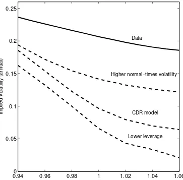
Figure 1.3 tests this directly by showing option prices in the CDR model for leverage of

5.1 and for leverage of 2.6 (denoted “lower leverage”) in the figure. Surprisingly, the slope

for the calibration with leverage of 2.6 is slightly higher than the slope for leverage of 5.1.

Lowering leverage results in a downward shift in the level of the implied volatility curve,

not the slope. Thus the difference in leverage cannot be the explanation for why the slope

in our model is lower than the slope for CDR.

Why does the change in leverage result in a shift in the level of the curve? It turns out that

in the CDR model, changing normal-times volatility has a large effect. Leverage affects

both the disaster distribution and normal-times volatility. Lowering leverage has a large

effect on normal-times volatility and thus at-the-money options. This is why the level of

the curve is lower, and the slope is slightly steeper.7

1.3.2. The role of normal shocks

To further consider the role of normal-times volatility, we explore the impact of changing

the consumption volatility parameterσ. In the benchmark CDR comparison, consumption

volatility is equal to the value of consumption volatility over the 1889–2009 sample, namely

3.5%. Most of this volatility is accounted for by the disaster distribution, because, while the

disasters are rare, they are severe. Therefore normal-times volatility is 1%, lower than the

(26)

differ-ently; following Barro (2006), the disaster distribution is determined based on international

macroeconomic data, and the normal-times distribution is set to match postwar volatility

in developed countries. The resulting normal-times volatility is 2%. To evaluate the effect

of this difference, we solve for implied volatilities in the CDR model with leverage of 5.1

and normal-times volatility of 2%. In Figure 1.3, the result is shown in the line denoted

“higher normal-times volatility.”

As Figure 1.3 shows, increasing the normal-times volatility of consumption growth in the

CDR model has a noticeable effect on implied volatilities: The implied volatility curve is

higher and flatter. The change in the level reflects the greater overall volatility. The change

in the slope reflects the greater probability of small, negative outcomes. However, the effect,

while substantial, is not nearly large enough to explain the full difference. The level of the

“higher normal-times volatility” smile is still too low and the slope is too high compared

with the data.8

While raising the volatility of consumption makes the CDR model look somewhat more like

the SDR model (though it does not account for the full difference), it is not the case that

lowering the volatility of consumption makes the SDR model more like the CDR model.

Namely, reducing σ to 1% (which would imply a normal-times consumption volatility that

is lower than in the post-war data) has almost no effect on the implied volatility curve

of the SDR model. There are two reasons why this parameter affects implied volatilities

differently in the two cases. First, the leverage parameter is much lower in the SDR model

than the CDR model. Second, volatility in the SDR model comes from time-variation in

discount rates (driven by λt) as well as in payouts (φσ). The first of these terms is much

larger than the second.9

8

Note further that leverage of 5.1, combined with a normal-times consumption volatility of 2% means that normal-times dividend volatility of dividends is 10.2%. However, annual volatility in postwar data is only 6.5%.

9_{To be precise, total return volatility in the SDR model equals the square root of the variance due to}

λt, plus the variance in dividends. Dividend variance is small, and it is added to something much larger to

(27)

1.3.3. The price of volatility risk

One obvious difference between the CDR model and the SDR model is that the SDR model

is dynamic. Because of recursive utility, this affects risk premia on options and therefore

option prices and implied volatilities. As shown in Section 1.2.2, the state price density

depends on the probability of disaster. Thus risk premia depend on covariances with this

probability: assets that increase in price when the probability rises will be a hedge. Options

are such an asset. Indeed, an increase in the probability of a rare disaster raises option prices,

while at the same time increasing marginal utility.

To directly assess the magnitude of this effect, we solve for option prices using the same

process for the stock price and the dividend yield, but with a pricing kernel adjusted to set

the above effect equal to zero. Risk premia in the model arise from covariances with the

pricing kernel. We replace the pricing kernel in (1.8) with one in which b= 0.10 Because b

determines the risk premium due to covariance withλt, settingb= 0 will shut off this effect.

Figure 1.4 shows, setting b= 0 noticeably reduces the level of implied volatilities, though

the difference between the b = 0 model and the SDR is small compared to the difference

between the CDR and the SDR model.

It is worth emphasizing that the assumption of b = 0 does not imply an iid model. This

model still assumes that stock prices are driven by stochastic disaster risk; otherwise the

volatility of stock returns would be equal to that of dividends.

1.3.4. The distribution of consumption growth implied by options

Our results show that a model with stochastic disaster risk can fit implied volatilities,

thereby addressing one issue raised by Backus, Chernov, and Martin (2011). Backus et

10

(28)

al. raise a second issue: assuming power utility and iid consumption growth, they back

out a distribution for the left tail of consumption growth from option prices (we will call

this the “option-implied consumption distribution”).11 Based on this distribution, they

conclude that the probabilities of negative jumps to consumption are much larger, and the

magnitudes much smaller, than implied by the international macroeconomic data used by

Barro (2006) and Barro and Ursua (2008).

The resolution of this second issue is clearly related to the first. For if a model (like the one

we describe) can explain average implied volatilities while assuming a disaster distribution

from macroeconomic data, then it follows that this macroeconomic disaster distribution is

one possible consumption distribution that is consistent with the implied volatility curve.

Namely, the inconsistency between the extreme consumption events in the macroeconomic

data and option prices is resolved by relaxing the iid assumption.

Of course, this reasoning does not imply that the stochastic disaster model is any better

than the iid model with the option-implied consumption distribution. This distribution is,

after all, consistent with option prices, the equity premium, and the mean and volatility of

consumption growth observed in the U.S. in the 1889-2009 period (provided a coefficient of

relative risk aversion equal to 8.7). However, it turns out that this consumption distribution

can be ruled out based on other data: because it assumes that negative consumption jumps

are relatively frequent (as they must be to explain the equity premium), some would have

occurred in the 60-year postwar period in the U.S. The unconditional volatility of

consump-tion growth in the U.S. during this period was less than 2%. Under the opconsump-tion-implied

consumption growth distribution, there is less than a 1 in one million chance of observing

a 60-year period with volatility this low.12

11

A methodological problem with this analysis is that it assumes that options are on returns rather than on prices. See footnote 5.

12

(29)

1.3.5. Summary

A consequence of stochastic disaster risk is high stock market volatility, not just during

occurrences of disasters, but during normal periods as well. This is reflected in the level

and shallowness of the volatility smile: while the existence of disasters leads to an upward

slope for out-of-the money put options, high normal-period volatility implies that the level

is high for put options that are in the money or only slightly out of the money. The same

mechanism, and indeed the same parameters that allow the model to match the level of

realized stock returns enable the model to match implied volatilities.

Previous work suggests that allowing for stochastic volatility (and time-varying moments

more generally) does not appear to affect the shape of the implied volatility curve.13 How

is it, then, that this paper comes to such a different conclusion? The reason may arise from

the fact that the previous literature mainly focused on reduced-form models, in which the

jump dynamics and volatility of stock returns are freely chosen. However, in an equilibrium

model like the present one, stock market volatility arises endogenously from the interplay

between consumption and dividend dynamics and agents’ preferences. While it is possible

to match the unconditional volatility of stock returns and consumption in an iid model,

this can only be done (given the observed data) by having all of the volatility occur during

disasters. In such a model it is not possible to generate sufficient stock market volatility

in normal times to match either implied or realized volatilities. While in the reduced-form

literature, the difference between iid and dynamic models principally affects the conditional

second moments, in the equilibrium literature, the difference affects the level of volatility

itself.

13

(30)

1.4. Option prices in a multi-factor stochastic disaster risk model

1.4.1. Why multiple factors?

The previous sections show how introducing time variation into conditional moments can

substantially alter the implications of rare disasters for implied volatilities. The model

pre-sented there was parsimonious, with a single state variable following a square root process.

Closer examination of our results suggests an aspect of options data that may be difficult

to fit to this model. Figure 1.5 shows implied volatilities forλtequal to the median and for

the 1st and 99th percentile value for put options with moneyness as low as 0.85.14 Implied

volatilities increase almost in parallel as λt increases. That is, ATM options are affected

by an increase in the rare disaster probability almost as much as out-of-the-money options.

The model therefore implies that there should be little variation in the slope of the implied

volatility curve.

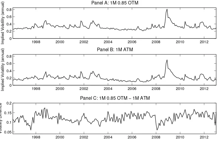
Figure 1.6 shows the historical time series of implied volatilities computed on one month

ATM and OTM options with moneyness of 0.85. Panel C shows the difference in the implied

probabilities, a measure of the slope of the implied volatility curve. Defined in this way,

the average slope is 12%, with a volatility of 2%. Moreover, the slope can rise as high as

18% and fall as low as 6%. While the SDR model can explain the average slope, it seems

unlikely that it would be able to account for the time-variation in the slope, at least under

the current calibration. Moreover, comparing Panel C with Panels A and B of Figure 1.6

indicates that the slope varies independently of the level of implied volatilities. Thus it is

unlikely that any model with a single state variable could account for these data.

The mechanism in the SDR model that causes time-variation in rare disaster probabilities

is identical to the mechanism that leads to volatility in normal times. Namely, when λt

14

(31)

is high, rare disasters are more likely and returns are more volatile. In order to account

for the data, a model must somehow decouple the volatility of stock returns from the

probability of rare events. This is challenging, because volatility endogenously depends on

the probability of rare events. Indeed, the main motivation for assuming time-variation in

the probability of rare events is to generate volatility in stock returns that seems otherwise

puzzling. Developing such a model is our goal in this section of the paper.

1.4.2. Model assumptions

In this section, we introduce a mechanism that decouples the volatility of stock returns from

the probability of rare events. We assume the same stochastic process for consumption (1.1)

and for dividends. We now assume, however, that the probability of a rare event follows

the process

dλt=κλ(ξt−λt)dt+σλ

p

λtdBλ,t, (1.13)

whereξt solves the following stochastic differential equation

dξt=κξ( ¯ξ−ξt)dt+σξ

p

ξtdBξ,t. (1.14)

We continue to assume that all Brownian motions are mutually independent. The process

for λt takes the same form as before, but instead of reverting to a constant value ¯λ, λt

reverts to a value that is itself stochastic. We will assume that this value, ξt itself follows

a square root process. Though the relative values of κλ and κξ do not matter for the

form of the solution, to enable an easier interpretation of these state variables, we will

choose parameters so that shocks toξt die out more slowly than direct shocks toλt. Duffie,

Pan, and Singleton (2000) use the process in (1.13) and (1.14) to model return volatility.

This model is also related to multi-factor return volatility processes proposed by Bates

(32)

our study, the process is for jump intensity rather than volatility; however, volatility, which

arises endogenously, will inherit the two-factor structure. While we implement a model with

two-factors in this paper, our solution method is general enough to encompass an arbitrary

number of factors with linear dependencies through the drift term, as in the literature on

the term structure of interest rates (Dai and Singleton (2002)).16

Like the one-factor SDR model, our two-factor extension is highly tractable. In

Ap-pendix A1.3.1, we show that utility is given by

Vt=

C_t1−γ

1−γe

a+bλλt+bξξt _(1.15)

where

a = 1−γ

β

µ− 1

2γσ

2

+bξκξ

¯

ξ

β (1.16)

bλ =

κλ+β

σ_λ2 −

s

κλ+β

σ_λ2

2

−2Eν

e(1−γ)Zt −₁

σ2_λ (1.17)

bξ =

κξ+β

σ2_ξ −

v u u

t κξ+β

σ_ξ2

!2

−2bλκλ

σ_ξ2 (1.18)

Equation 1.5 still holds for the state-price density, though the process Vt will differ. The

riskfree rate and government bill rate are the same functions of λt as in the one-factor

model. In Appendix A1.3.3, we show that the price-dividend ratio is given by

G(λt, ξt) = exp (aφ(τ) +bφλ(τ)λt+bφξ(τ)ξt), (1.19)

16

(33)

whereaφ,bφλ and bφξ solve the differential equations

a0_φ(τ) = −β−µ−γ(φ−1)σ2+µD +bφξ(τ)κξξ¯

b0_φλ(τ) = −b_φλ(τ)κλ+ 1

2bφλ(τ)

2_σ2

λ+bλbφλ(τ)σλ2+Eν

h

e(φ−γ)Zt₋_e(1−γ)Zt i

b0_φξ(τ) = −b_φλ(τ)κλ−bφξ(τ)κξ+ 1

2bφξ(τ)

2_σ2

ξ +bξbφξ(τ)σξ2,

with boundary condition

aφ(0) =bφλ(0) =bφξ(0) = 0.

Similar reasoning to that of Section 1.2.3 shows that for a given moneyness and time to

expiration, normalized option prices and implied volatilities are a function of λt and ξt

alone. To solve for option prices, we approximate G(λt, ξt) by a log-linear function of λt

and ξt, as shown in Appendix A1.3.3.

1.5. Fitting the multifactor model to the data

1.5.1. Parameter choices

For simplicity, we keep risk aversion γ, the discount rate β and the leverage parameter φ

the same as in the one-factor model. We also keep the distribution of consumption in the

event of a disaster the same. Note that κλ and σλ will not have the same interpretation in

the two-factor model as κ andσλ do in the one-factor model.

Our first goal in calibrating this new model is to generate reasonable predictions for the

aggregate market and for the consumption distribution. That is, we do not want to allow

the probability of a disaster to become too high. One challenge in calibrating representative

agent models is to match the high volatility of the price-dividend ratio. In the two-factor

model, as in the one-factor model, there is an upper limit to the amount of volatility

(34)

respective volatilities must be so as to ensure that the discriminants in (1.17) and (1.18)

stay nonnegative. We choose parameters so that the discrimant is equal to zero; thus there

is only one more free parameter relative to to the one-factor model.

The resulting parameter choices are shown in Table 1.2. The mean reversion parameterκλ

and volatility parameterσλ are relatively high, indicating a fast-moving component to the

λt process, while the mean reversion parameter κξ and σξ are relatively low, indicating a

slower-moving component. The parameter ¯ξ (which represents both the average value ofξt

and the average value ofλt) is 2% per annum. This is lower than ¯λin our calibration of the

one-factor model. In this sense, the two-factor calibration is more conservative. However,

the extra persistence created by theξtprocess implies thatλtcould deviate from its average

for long periods of time. To clarify the implications of these parameter choices, we report

population statistics onλtin Panel C of Table 1.2. The median disaster probability is only

0.37%, indicating a highly skewed distribution. The standard deviation is 3.9% and the

monthly first-order autocorrelation is 0.9858.

Implications for the riskfree rate and the market are shown in Table 1.3. We simulate

100,000 samples of length 60 years to capture features of the small-sample distribution.

We also simulate a long sample of 600,000 years to capture the population distribution.

Statistics are reported for the full set of 100,000 samples, and the subset for which there are

no disasters (38% of the sample paths). The table reveals a good fit to the equity premium

and to return volatility. The average Treasury Bill rate is slightly too high, though this

could be lowered by lowering β or by lowering the probability of government default.17

The model successfully captures the low volatility of the riskfree rate in the postwar period.

The median value of the price-dividend ratio volatility is lower than in the data (0.27 versus

0.43), but the data value is still lower than the 95th percentile in the simulated sample.18

For the market moments, only the very high AR(1) coefficient in postwar data falls outside

17

As in the one-factor model, we assume a 40% probability of government default.

18_{The one-factor model, which was calibrated to match the population persistence of the price-dividend}

(35)

the 90% confidence bounds: it is 0.92 (annual), while in the data, the median is 0.79 and the

95th percentile value is 0.91. As we will show below, there is a tension between matching

the autocorrelation in the price-dividend ratio and in option prices. Moreover, so that

utility converges, there is a tradeoff between persistence and volatility. One view is that the

autocorrelation of the price-dividend ratio observed in the postwar period may in fact have

been very exceptional and perhaps is not a moment that should be targeted too stringently.

1.5.2. Simulation results for the two-factor model

We first examine the fit of the model to the mean of implied volatilities in the data. We

ask more of the two-factor model than its one-factor counterpart. Rather than looking only

at 3-month options across a narrow moneyness range, we extend the range to options of

moneyness of 0.85. We also look at 1- and 6-month options, and at moments of implied

volatilities beyond the means. Moreover, rather than looking only at the population average,

we consider the range of values we would see in repeated samples that resemble the data,

namely, samples of length 17 years with no disaster. This is a similar exercise to what was

performed in Table 1.3, though calculating option prices is technically more difficult than

calculating equity prices.19

Figure 1.7 shows means and volatilities of implied volatilities for the three option maturities.

We report the averages across each sample path, as well as 90% confidence intervals from

the simulation. We see that this new model is successful at matching the average level

of the implied volatility curve for all three maturities, even with this extended moneyness

range, and even though we are looking at sample paths in which the disaster probability

will be lower than average. In fact the slope in the model is slightly below that in the data.

Similarly, the model’s predictions for volatility of volatility are well within the standard

error bars for all moneyness levels and for all three option maturities.

19

(36)

One issue that arises in fitting both options and equities with a single model is the very

different levels of persistence in the option and equity markets. This tension is apparent

in our simulated data as well. As Table 1.3 reports, the annual AR(1) coefficient for the

price-dividend ratio in the data is extremely high: 0.92; just outside of our 10% confidence

intervals. The median value from the simulations is still a very high 0.79; in monthly

simulations, this value is 0.98. Implied volatilities in simulated data have much lower

autocorrelations. Median autocorrelations are roughly the same across moneyness levels,

and are in the 0.92 to 0.94 range; substantially below the level for the price-dividend ratio.

The AR(1) coefficients in the data are lower still, though generally within the 10% confidence

intervals.20 While the same two factors drive equity and option prices, they do so to different

extents. The model endogenously captures the greater persistence in equity prices, which

represent value in the longer run than do option prices.

1.5.3. Implications for the time series

We now return to the question of whether the two-factor model can explain time-variation

in the slope and the level of option prices. Before embarking on this exercise we note that

the matching the time series is not usually a target for general equilibrium models because

these models operate under tight constraints. We expect that there will be some aspects of

the time series that our model will not be able to match.

We consider the time series of one-month ATM and OTM implied volatilities (Figure 1.6).

For each of these data points, we compute the implied value of λt and ξt. Note that this

exercise would not be possible if the model were not capable of simultaneously matching the

level and slope of the implied volatility curve for one-month options. We show the resulting

values in Figure 1.8. For most of the sample period, the disaster probability λt varies

between 0 and 6%, with spikes corresponding to the Asian financial crisis in the late 1990s

and the large market declines in the early 2000s. However, the sample is clearly dominated

20

(37)

by the events of 2008-2009, in which the disaster probability rises to about 20%. 21 While we choose the state variables to match the behavior of one-month options exactly, Figure 1.9

shows that the model also delivers a good fit to the time series of implied volatilities from

three-month and six-month options.

The exercise above raises the question of whether the time series of λt and ξt are

reason-able given our assumptions on the processes for these varireason-ables. Treason-able 1.4 calculates the

distribution of moments for λtand ξt. With the exception of the first-order autoregressive

coefficients, the data fall well within the 90% confidence intervals. That is, the average

values of the state variables and their volatilities could easily have been observed in

17-year samples with no disasters. The persistence in the data is somewhat lower than the

persistence implied by the model. This illustrates the same tension between matching the

time series of option prices and the time series of the price-dividend ratio discussed in the

previous section.

As discussed in Section 1.4.1, it is not clear why adding a second state variable would allow

the model to capture the time series variation in both the level and the slope, since both

of these observables would be endogenously determined by both state variables. To better

understand the mechanisms that allow the model to match these data, we consider the

relative contributions of two state variables to the implied volatility curve in Figure 1.10.

Panel A of Figure 1.10 fixes ξt at its median value and shows implied volatilities for λt

at its 80th percentile value, at its median, and at its 20th percentile value. Panel B of

Figure 1.10 performs the analogous exercise, this time fixingλtbut varyingξt. In contrast

to its behavior in the one-factor model, increasing λt both increases implied volatilities

and increases the slope. The state variable ξt has a smaller effect on the level of implied

volatilities, but a greater effect on the slope. Moreover, an increase in ξt lowers the slope

rather than raising it. To summarize, increases in λt raise both the level and the slope of

(38)

the implied volatility curve. Increases inξtslightly raise the level and decrease the slope.

Why does ξt affect the slope of the implied volatility curve? The reason is that ξt has

a relatively small effect on the probability of disasters at the time horizon important for

option pricing, but a large effect on the volatility of stock prices (because of the square root

term on its own volatility). Thus increases in ξt flatten the slope of the implied volatility

curve because they raise the implied volatility for ATM options much more than for OTM

options. The process forλt, on the other hand, has a large effect on OTM implied volatilities

because it directly controls the probability of a disaster. It has a smaller effect on ATM

implied volatilities than in the one-factor model because of its lower persistence.

Finally, we ask what these implied volatilities say about equity valuations. Given the

option-implied values of ξ and λ, we can impute a price-dividend ratio using (1.19). This

price-dividend ratio uses no data on equities, only data on options and the model. Figure

Figure 1.12 shows the results, along with the price-dividend ratio from data available from

Robert Shiller’s webpage. The model can match the sustained level of the price-dividend

ratio, and, most importantly, the time series variation after 2004.22 Indeed, between 2004

and 2013, the correlation between the option-implied price-dividend ratio and the actual

price-dividend ratio is 0.84, strongly suggesting these two markets share a common source

of risk.

1.5.4. The implied volatility surface

We now take a closer look at what the model says about the implied volatility surface,

namely implied volatilities across moneyness and time to expiration. Figures 1.11 show

the implied volatilities for one, three and six-month options as a function of moneyness.

We show the average implied volatilities computed using the time series of λt and ξt, and

compare these to the data. Given that we have chosenλt and ξt to match the time series

of implied volatilities on 1-month options, it is not surprising that the model matches these

22

(39)

data points exactly. More interestingly, the model is able to match the three-month and

the six-month implied volatility curves almost exactly, even though it was not calibrated to

these curves.

The downward slope in implied volatilities from options expiring in as long as six months

indicates that the risk-neutral distribution of returns exhibits considerable skewness at long

horizons. This is known as the skewness puzzle (Bates (2008)) because the law of large

numbers would suggest convergence toward normality as the time to expiration increases.

Recently, Neuberger (2012) makes use of options data to conclude that the skewness in the

physical distribution of returns is also more pronounced than has been estimated previously.

Neuberger emphasizes the observed negative correlation between stock prices and volatility

(French, Schwert, and Stambaugh (1987)) as a reason why skewness in long-horizon returns

does not decay as the law of large numbers in an iid model suggests that it would (see also

Bates (2000)).

Figures 1.7 and 1.11 show that our model can capture the downward slope in 6-month

implied volatilities as well as the slope for shorter-term options. Thus stock returns in

the model exhibit skewness at both long and short-horizons. The short-horizon skewness

arises from the existence of rare disasters. Long-horizon skewness, however, comes about

endogenously because of the time-variation in the disaster probability. An increase in the

rare disaster probability leads to lower stock prices, and, at the same time, higher volatilities,

thereby accounting for this co-movement in the data. As a result, returns maintain their

skewness at long horizons, and the model can explain six-month as well as one-month

implied volatility curves.

1.6. Conclusion

Since the early work of Rubinstein (1994), the implied volatility curve has constituted an

(40)

The implied volatility curve, almost by definition, has been associated with excess kurtosis in

stock prices. Separately, a literature has developed linking kurtosis in consumption (which

would then be inherited by returns in equilibrium) with the equity premium. However,

much of the work up to now, as exemplified by a recent paper by Backus, Chernov, and

Martin (2011) suggests that, at least for standard preferences, the non-normalities required

to match the equity premium are qualitatively different from those required to match implied

volatility.

We have proposed an alternative and more general approach to modeling the risk of

down-ward jumps that can reconcile the implied volatility curve and the equity premium. Rather

than assuming that the probability of a large negative event is constant, we allow it to

vary over time. The existence of very bad consumption events leads to both the downward

slope in the implied volatility curve and the equity premium. Moreover, the time-variation

in these events moderates the slope, raises the level and generates the excess volatility

observed in stock prices. Thus the model can simultaneously match the equity premium,

equity volatility, and implied volatilities on index options. Option prices, far from ruling

out rare consumption disasters, provide additional information for the existence of what

has been referred to as the “dark matter” of asset pricing (Campbell (2008), Chen, Dou,

and Kogan (2013)).

The initial model that we develop in the paper is deliberately simple and parsimonious.

However, there are some interesting features of option and stock prices that cannot be

matched by a model with a single state variable; for example, the imperfect correlation

between the slope and the level of the implied volatility curve. For this reason, we

inves-tigate a more general model that allows for variation in disaster risk to occur at multiple

time scales. This modification naturally produces time-variation in the slope of implied

volatilities because it introduces variation in stock price volatility that can be distinguished

from the risk of rare disasters. Taken together, these results indicate that options data

(41)

data can provide information about the disaster distribution beyond that offered by stock

prices. In particular, data from options suggest that modeling time-variation in disaster

(42)

Figure 1.1: Probability density functions for consumption declines

0 10 20 30 40 50 60 70 80

0 0.5 1 1.5 2 2.5 3 3.5 4 4.5 5

Percent decline on consumption

Probability density

Multinomial disasters

Lognormal disasters

Notes: The probability density functions (pdfs) for consumption declines for log-normally distributed disasters and for the multinomial distribution assumed in the stochastic disaster risk (SDR) model. In the case of the SDR model, the pdf approximates the multinomial distribution from Barro and Ursua (2008). The exact multinomial distribution is used to

(43)

Figure 1.2: Average implied volatilities in the SDR and CDR models

0.940 0.96 0.98 1 1.02 1.04 1.06

0.05 0.1 0.15 0.2 0.25

Moneyness

Implied Volatility (annual)

Data

SDR model

CDR model

(44)

Figure 1.3: Comparative statics for the CDR model

0.940 0.96 0.98 1 1.02 1.04 1.06

0.05 0.1 0.15 0.2 0.25

Moneyness

Lower leverage CDR model Data

Higher normal−times volatility

(45)

Figure 1.4: Evaluating the role of recursive utility

0.940 0.96 0.98 1 1.02 1.04 1.06

0.05 0.1 0.15 0.2 0.25

Moneyness

SDR model

SDR model with b = 0

Data

CDR model

Notes: Implied volatilities for 3-month options as a function of moneyness in the data, in the CDR model (calibrated as in Table 1.1) and in the SDR model. Also shown are implied volatilities in the SDR model computed under the assumption that the premium associated

with time-variation in the disaster probability is equal to zero (SDR model with b = 0).

Note both the benchmark and the b = 0 version of the SDR model are dynamic models

(46)

Figure 1.5: Implied volatilities for given values of the disaster probability

0.86 0.88 0.9 0.92 0.94 0.96 0.98 1 1.02

0 0.1 0.2 0.3 0.4 0.5 0.6

Moneyness

Data − 99th percentile Model − 99th percentile

Data − median

Data − 1st percentile Model − median

Model − 1st percentile

(47)