Complementary pathways to sustainability

(1)

Research Report: Number 11/04

Complementary pathways to sustainability

Lesley Hunt

with assistance from Dave Lucock, Glen Greer, Peter Carey, Jayson

Benge, Henrik Moller, Jon Manhire, Chris Rosin, Catriona MacLeod,

and other members of the ARGOS team since its inception in 2003

December 2011

(2)

Pathways to Sustainability

Acknowledgements

This work was funded by the Foundation for Research, Science and Technology (Contract Number AGRB0301).

(3)

List of Tables

Table 2.1: Summary of core variables used ... 16

Table 3.1: Correlations of averages of core variables ... 58

Table 3.2: Correlations of annual trends of core variables ... 59

Table 3.3: Table: Correlations of variation (s.d.s) of core variables ... 60

Table 3.4: Annual change in core variables for all ARGOS orchards ... 61

Table 3.5 Rotated Principal Components for averages of core variables ... 62

Table 3.6: Cluster analysis groups of averages of core variables ... 62

Table 3.7: Characteristics of the groups from the cluster analysis of the averages of core variables ... 63

Table 3.8: Characteristics of the groups from cluster analysis of averages of core variables, in terms of annual trend/change of core variables ... 64

Table 3.9: Characteristics of the groups from cluster analysis of averages, in terms of variation (s.d.) of core variables ... 64

Table 3.10: Other variables to add to descriptions of groups clustered from averages of core variables .. 65

Table 3.11: Characteristics of the groups from cluster analysis of averages, in terms bird densities ... 66

Table 3.12: Characteristics of the groups from cluster analysis of averages, in terms attitude variables (from 2008 survey) ... 66

Table 3.13: The impact of management system, orchard size and location on the differences between the groups of the averages of the core variables ... 69

Table 3.14: Principal Components of annual change of core variables... 69

Table 3.15: Cluster analysis groups formed on principal component scores of annual change of core variables ... 70

Table 3.16: Characteristics of the groups from cluster analysis, using annual change in core variables .. 70

Table 3.17: Characteristics of the groups from cluster analysis of annual change of core variables, in terms of averages of core variables (Are orchardists who are not changing already at a high level of intensification, capital and efficiency?) ... 71

Table 3.18: Characteristics of the groups from the cluster analysis on change, using the variation (s.d.) of core variables ... 71

Table 3.19: Other variables to add to descriptions of groups clustered from annual change of core variables ... 72

Table 3.20: Bird density ... 72

Table 3.21: Attitude variables (from 2008 survey) ... 73

Table 3.22: Rotated Principal Components for variation of core variables ... 74

Table 3.23: Cluster analysis groups of variation of core variables ... 74

Table 3.24: Characteristics of the groups from cluster analysis of the variation of core variables ... 75

Table 3.25: Characteristics of the groups from cluster analysis of variation of core variables, in terms of averages of core variables (Are orchardists who are the most consistent already at a high level of intensification, capital and efficiency?) ... 75

Table 3.26: Characteristics of the groups from cluster analysis of variation of core variables, in terms of annual trend/change of core variables ... 76

(6)

Table 3.28: Characteristics of the groups from cluster analysis of variation of core variables, in terms of

bird density ... 78

Table 3.29: Characteristics of the groups from cluster analysis of variation of core variables, in terms of attitude variables (from 2008 survey)... 78

Table 4.1: Correlations of averages of core variables ... 80

Table 4.2: Correlations of annual trends of core variables ... 81

Table 4.3: Correlations of variation (s.d.) of core variables ... 82

Table 4.4: PCA analysis of averages of core variables ... 83

Table 4.5: Cluster analysis of averages of core variables ... 83

Table 4.6: Characteristics of the groups from the cluster analysis of the averages of core variables ... 84

Table 4.7: Characteristics of groups from cluster analysis of averages of core variables, in terms of annual trend/change of core variables ... 85

Table 4.8: Characteristics of groups from cluster analysis of averages of core variables, in terms of variation of core variables ... 85

Table 4.9: Financial return and expenses ($) analysed across groups formed from averages ... 86

Table 4.10: Characteristics of groups formed from averages in terms of bird density (measurements over three years: 2004-5, 2007-8, 2009-2010) ... 88

Table 4.11: Characteristics of groups formed from averages in terms of fertiliser applied and additional soil measurements ... 89

Table 4.12: Characteristics of groups formed from averages in terms of other farm management variables ... 90

Table 4.13: Characteristics of groups formed from averages in terms of attitude variables (from 2008 survey)... 91

Table 4.14: PCA analysis of annual change in core variables ... 94

Table 4.15: Cluster analysis of annual change in core variables ... 94

Table 4.16: Characteristics of the groups from the cluster analysis of annual change of core variables ... 95

Table 4.17: Characteristics of the groups from cluster analysis of annual change of core variables, in terms of averages of core variables ... 95

Table 4.18: Characteristics of the groups from cluster analysis of annual change of core variables, in terms of variation of core variables ... 96

Table 4.19: Characteristics of groups formed from annual change in terms of financial expenses ... 96

Table 4.20: Characteristics of groups formed from annual change in terms of bird density (measurements over three years: 2004-5, 2007-8, 2009-2010) ... 97

Table 4.21: Characteristics of groups formed from annual change in terms of fertiliser applied and additional soil measurements ... 97

Table 4.22: Characteristics of groups formed from annual change in terms of other farm management variables ... 98

Table 4.23: Characteristics of groups formed from annual change in terms of attitude variables (from 2008 survey)... 99

Table 4.24: PCA analysis of variation of core variables... 100

Table 4.25: Cluster analysis of variation of core variables ... 100

Table 4.26: Characteristics of the groups from the cluster analysis of the variation of core variables ... 101

(7)

Table 4.28: Characteristics of the groups from cluster analysis of variability of core variables, in terms of

annual trend/change of core variables ... 102

Table 4.29: Characteristics of groups formed from variation in terms of financial expenses ... 103

Table 4.30: Characteristics of groups formed from variation in bird density (measurements over three years: 2004-5, 2007-8, 2009-2010) ... 104

Table 4.31: Characteristics of groups formed from variation in terms of fertiliser applied and additional soil measurements ... 104

Table 4.32: Characteristics of groups formed from variation in terms of other farm management variables ... 105

Table 4.33: Characteristics of groups formed from variation in terms of attitude variables (from 2008 survey)... 105

Table 4.34: Correlations of averages of core variables (without cropping) ... 107

Table 4.35: Correlations of annual trends of core variables (without cropping) ... 108

Table 4.36: Correlations of variation (s.d.) of core variables (without cropping) ... 109

Table 4.37: PCA analysis of averages of core variables (without cropping) ... 110

Table 4.38 2: Cluster analysis of averages of core variables (without cropping) ... 110

Table 4.39: Characteristics of the groups from the cluster analysis of the averages of core variables (without cropping) ... 111

Table 4.40: Characteristics of the groups from cluster analysis of averages of core variables, in terms of annual trend/change of core variables (without cropping) ... 112

Table 4.41: Characteristics of the groups from cluster analysis of averages of core variables, in terms of variation of core variables (without cropping) ... 112

Table 4.42: Characteristics of groups formed from averages in terms of financial expenses (without cropping) ... 113

Table 4.43: Characteristics of groups formed from averages in terms of bird density (measurements over three years: 2004-5, 2007-8, 2009-2010) ... 114

Table 4.44: Characteristics of groups formed from averages in terms of fertiliser applied and additional soil measurements ... 115

Table 4.45: Characteristics of groups formed from averages in terms of other farm management variables ... 116

(8)

Acronyms

anova - analysis of variance

COS - cash orchard surplus = income minus operating expenditure

C & NC feed – cash and non-cash supplements

C & NC Labour – cash and non-cash labour

DM – dry matter (kiwifruit orchardists receive premiums for achieving high levels of DM)

EOS - Economic Orchard Surplus (difference between income and expenditure which has an adjustment for soil P and unpaid labour)

EFS - Economic Farm Surplus (difference between income and expenditure which has an adjustment for unpaid labour)

FWE – Farm Working Expenses

FWE/GFR - Farm Working Expenses divided by Gross Farm Revenue (a measure of the ‘efficiency’ of the farm because it measures the proportion of the revenue that is spent on the workings of the farm.

GOR = Gross Orchard Revenue (income)

Ha – hectares

NFPBT – Net Farm Profit Before Tax

OWE - Orchard Working Expenses

OWE/GOR – Orchard Working Expenses divided by Gross Orchard Revenue (a measure of the ‘efficiency’ of the orchard because it measures the proportion of the revenue that is spent on the workings of the orchard.

PCA – Principal Components Analysis

SU – stock units

(9)

1 Introduction and rationale

The ARGOS programme is a study of New Zealand sheep/beef and dairy farms and kiwifruit orchards that examines the sustainability and resilience of New Zealand’s farming - economically, socially and environmentally. In completing ARGOS1, additional and more intractable sustainability concerns (e.g. climate change and carbon emissions, RMA, animal welfare) have been identified by both the preliminary research and through discussion with industry partners, as key emerging pressures on management practices. In such cases, the pathways to enhanced performance are not exclusively organised around market assurance schemes, but are often structured around regulatory responses, eliciting a separate and substantial set of economic, social and environmental impacts in the primary production sector to that studied in ARGOS1. In addition, cross-cultural comparisons among ARGOS participants has demonstrated the often-essential role of differing philosophical approaches to agricultural practice, which affect the mix of concerns (environmental, social and economic) that influence management actions. To account for the broader spectrum of pathways that influence management, ARGOS 2 will examine the characteristics and outcomes of various pathways to sustainability. This will include an in-depth analysis of intensification of production as an example of a type of response to complementary pathways and the impact on sustainability. The results will be reviewed to clarify the relative effectiveness of the various pathways and tools on farmer behaviour, environmental outcomes and meeting stakeholder’s expectations.

1.1 ARGOS 1

The work of ARGOS has mainly been involved in two sectors – kiwifruit and sheep/beef. The kiwifruit study has been of 36 orchards at 12 locations - Kerikeri (1), Bay of Plenty (10) and Motueka (1). At each location there are three ARGOS orchards under management systems associated with growing green, gold and organic green kiwifruit. For the sheep/beef study there are 36 farms based at 12 different locations throughout the South Island. At each location there are three farms using conventional, integrated and organic management systems. However, in ARGOS 2.1, we have moved on to study the sustainability of these orchards and farms independent of management system.

Up until 2009 the ARGOS study (ARGOS 1) has been concerned with comparing the difference between management practices associated with audit systems in the kiwifruit, sheep/beef and dairy sectors of New Zealand’s agriculture. Now in ARGOS 2.1 we are concentrating on how famers have changed their farming practices and why.

1.2 ARGOS 2.1

1.2.1 Summarising the results from the retrospective interviews: complementary pathways to sustainability

The first part of ARGOS 2.1 has been based on retrospective interviews of ARGOS famers and orchardists which were conducted to find out how they dealt with shocks over their time in farming (Sanne et al., 2011a) and orcharding (Sanne et al., 20011b). This work also revealed the different pathways farmers and orchardists had taken to manage and overcome shocks that had impacted on their farming and orcharding systems.

(10)

lower returns they have been receiving for their animal-based products – resulted in many farmers making changes which gave them greater flexibility to respond to future shocks and diversified their product range. This flexibility is such that ARGOS farms reveal no common patterns of meat production – variability being the norm.

The tenure review process is having a negative impact High Country farmers, mainly due to the length of time taken for individual farms to get through the process (see Hunt et al., 2012). It provides an example of how government policy needs to be clear from the start, consistent and fair to all, and managed in a timely fashion. Long-term policies need to have obtained some consensus between government parties before their implementation.

The single desk marketing organisation ZESPRI has managed a robust kiwifruit industry which has enabled different kinds of people to participate with a sense of satisfaction. However the sustainability of the industry is challenged by the coming together of several challenges – psa, the declining market value of Hayward green kiwifruit and the value of land.

1.2.2 Implementation pathways: changing practices to manage risk and enhance chances of survival

Elements of sheep/beef farmers’ pathways to sustainability on-farm included: • Increasing lambing percentages by breeding genetics.

• Scanning pregnant ewes to better manage nutritional requirements.

• Stocking rate flexibility - destocking at certain times of the year to manage anticipated drought periods, by earlier lambing, faster lamb growth through better feed etc., trading in stock to manage feed availability.

• Keeping greater stocks of silage, baleage and growing feed crops, to have on hand sufficient feed for winter or drought periods.

• Increasing farm size by purchase or lease of land to provide a run-off for summer. • Adding irrigation, or increasing the area already irrigated.

• Diversification – changing the balance of sheep and cattle, providing dairy support, growing for meat rather than wool, growing contract crops only, animal trading. • Reducing fuel consumption by employing low till techniques.

• Belt tightening – reducing fertiliser input, reducing costs. • Focusing on efficiency - seeing farm as a business.

Off-farm elements included:

• Off-farm work. (Female partners often work in their own right and though this may not be to complement the farm’s finances, it does this none-the-less.)

• Restructuring of finances. Many wanted to earn sufficient income to help them prepare for succession by investing off-farm.

(11)

through a long period of poor market returns, High Country farmers are taking a particular pathway to sustainability through:

• Diversification - producing both meat (merino lambs and beef) and fine wools, developing a niche market for merino meat.

• Intensification - finishing stock themselves on irrigated and cultivated land, growing their own supplementary feed crops.

• Long term contracts of 3- 5 years for fine wool with companies like Icebreaker, with whom farmers develop personal relationships.

In the Kiwifruit industry ZESPRI leads from the front and orchardists follow: The kiwifruit

retrospective interviews were carried out before the discovery of PSA on orchards. Pathways to sustainability have been imposed by ZESPRI as it has responded to what they have viewed as market demands. In return orchardists have responded to these demands with their own pathways. These have included:

• Off-orchard work – which is more readily available in the areas where kiwifruit is grown. • Response to labour shortage by changing pruning techniques.

• Response to Taste ZESPRI by the development of controversial vine girdling techniques. Some orchardists are not practicing them or now reducing this practice because of

concern about the impact on vine health long-term.

• Continued support for the single desk structure of ZESPRI.

• Response to GlobalG.A.P.is now incorporated into practice after initial fears of some orchardists about being restricted to book work. For younger orchardists such audit practices are just part of being a contemporary business.

• Response to KiwiStart is mixed. This was expressed as concern about the quality of early season fruit.

1.2.3 Recommendations

From the analysis of the retrospective interviews it is suggested that:

• Farmers and orchardists want to ‘do the right thing’ and expect in exchange that the ‘right thing’ will be done to them.

• The autonomy of farmers and orchardists should be respected. They need to be given choices not commands, goals and various ways of getting there.

• There is a need a diversity of practices acceptable to orchardists and farmers so they can choose and match their practices to the situation they find themselves in.

• Recommended practices should demonstrate – possibly visually – what a ‘good’ farmer or orchardist someone is. (This is part of establishing a reputation and hence being trusted in the industry community.)

• Where possible industry partners should form personal relationships with farmers and orchardists, keeping them in touch with the quality of their products, promoting loyalty and pride in their product (e.g., Icebreaker).

• There needs to be an awareness of the different seasonal opportunities in contracts dependent on location (e.g., KiwiStart).

• It would be more useful to farmers and orchardists to have contracts that provide continuity over several years (e.g., Icebreaker, and dairy and kiwifruit – minimum payments and top ups later).

(12)

social and environmental view (awareness of reach of impacts of practices economically, socially and environmentally), and alternative practices.

1.2.4 Findings in the context of New Zealand and international research

There is international interest in the way ARGOS is comparing organic farming with other management practices. This places organic farming in a broader context in which it influences and is influenced by the practices of other management systems to increase the sustainability and resilience of the agricultural sector as a whole (Hunt et al., 2011). The ‘good farming’ approach used by ARGOS researchers, in which it is assumed that farmers have an inherent desire to fit into culturally acceptable ways of practicing farming, is a new way of thinking about farming in comparison to the standard farm management literature (e.g., Hunt, 2010).

1.2.5 This report: review of ARGOS results to clarify the relative effectiveness of the various pathways and tools for promoting change

This present report now examines the complementary pathways (apart from audit) that the ARGOS kiwifruit orchardists and sheep/beef farmers have taken to ensure they have survived through the time of the ARGOS study so far (2003 to 2011). It does this by examining statistically the hard data gathered over the period of ARGOS (2003 to 2010) from all aspects of the ARGOS research. That is it uses farm management, environmental, economic and social data.

ARGOS now has data that covers a reasonable period of time. It was decided that an exploration of how the ARGOS farms and orchards have changed over that time and what that change might be associated with would reveal what pathways farmers and orchardists have taken to survive through the past eight years. Farmers/orchardists may already be doing certain things well as they thought they could, and so be seeking to maintain those things rather than improve on them, so it was realised that the analysis needed to study absolute values over time (variable means) as well as change. The first analysis was of the kiwifruit data as the sheep/beef farming system is rather more complex and a first look at the meat production data showed complete variability over the past few years. That is, farmers were constantly adjusting their systems in terms of how many stock they finished/sold/bought etc. This introduced another way of looking at the data – how variable was it? Were farmers and orchardists constantly adjusting their practices or were they doing the same thing year after year? The obvious analysis was to find whether there were different patterns of practice followed by groups of farmers/orchardists which were resulting in differing outcomes over the time of the ARGOS study so far.

Pathways to sustainability indicate resilience over time. Core variables were chosen to develop groupings of farmers and orchardists that would hold together to form separate indices of resilience associated with intensification, capital value, efficiency and sustainability. Cluster analyses on a reduced number of variables composed from principal components analysis produced different groupings of farmers and orchardists associated with averages, change and variability of the core variables. Further characteristics of these groups were then found by analysis using as many relevant variables from the ARGOS research.

(13)

2 Method

What follows is a full description of the methods used and the decisions made to analyse this comprehensive ARGOS data set. This is not usual and many readers may wish to skip to the next chapter of the report. It is included because the author wishes to make clear all the decisions that were made in this analysis to indicate that statistical analysis is not the objective exercise it usually purports to be in the scientific literature. All numbers and analyses involve choices made by the data collectors and the analysts of that data, and all analyses need to be interpreted by people who draw on their understanding of the data and its background.

2.1 An index approach?

After discussion at an ARGOS meeting in August, 2011, when people added variables that they thought should be included in the core analysis, it was decided to construct indices of intensification, capital, efficiency and sustainability through using averages, measures of the annual rate of change (slope of regression line per year) and variability for each of the core variables. However when these variables did not work as single indices for the initial sheep/beef analysis, the approach to the kiwifruit data was adjusted - still focusing on these concepts but doing separate analyses for the average, trend and variability data.

2.2 To standardise and if so what to standardise?

At first each variable was adjusted to try to get a measure that was comparable across management systems. This was done by standardising each variable within each management system. However, it was realised that the interest of this research was focused on pathways to resilience and sustainability and therefore any analysis should be independent of management system. Some key questions are which farms were producing enough in a sustainable way to make them resilient, what changes were being made and how consistent were farmers over the years? Therefore there was no need to standardise the variables to remove the effect of management system. In addition, the procedure for Principal Components Analysis (PCA), if based on correlation matrices, did not need to use standardised variables, so the raw variables were the basis of the analyses.

2.3 Measuring variation

At first it was suggested that the Coefficient of Variation1 (CV) should be used as a measure of variation within each variable. However, this works well in a scientific data set containing measures of physical phenomena, but the ARGOS data set contains financial variables which can cover a wide variation and sometimes occur as a loss – in other words, they had a negative value. This means that sometimes the mean averages out to be a very small figure approaching zero, while the variation can be quite large in comparison, which makes the CV a very large value approaching infinity! Therefore, it was decided to use the standard deviation (s.d.) as a more consistent and useful measure of the variation of a variable in this situation.

(14)

2.4 Choice of kiwifruit variables

A Principal Components Analysis requires a full data set with no missing data. This placed a limit on which variables were available to be chosen as the core variables for the initial PCA analysis and also constrained the number of orchards which could be included.

As measures of ‘intensification’ the variables used were: • Economic Orchard Surplus per hectare (EOS/ha), • Cash Orchard Surplus/ha (COS/ha),

• trays of fruit produced2 , and

• percentage of orchard canopy area producing Green (Hayward) fruit.

Included in ARGOS is a panel of Gold (Hort16a variety) orchards but some of these orchards are also growing Green kiwifruit (Hayward variety). From earlier analyses and interviews the ARGOS team has determined that the orchardists who grow only gold fruit tend to be different from those that grow both gold and green, the latter being more conservative in their practices and in their propensity for risk taking, being more like the orchardists who grow only green fruit. Hence the latter variable, percentage of canopy producing Green fruit, can be thought of as a measure of intensification because a Gold canopy area produces more kiwifruit on average than the same area of Green canopy.

On the advice of Jayson Benge, the ARGOS kiwifruit field research manager, measures of ‘capital’ used were:

• the canopy area of the orchard, and

• soil resource measured by pH, Olsen P, percentage nitrogen (N%), potassium (K) and sulphur (S).

Kiwifruit production is improved by the addition of potassium and sulphur to the soil so if the soil has a good measure of these soil attributes it can be valued as a capital resource. Equity could also be regarded as a measure of capital but it was only available for about half of the orchards3 which would have reduced the number of orchards able to be used in the PCA analysis, so this variable was not used as part of the core analysis.

Measures of ‘efficiency’ were:

• the ratio of the Cash Orchard Expenses to Gross Orchard Revenue (COE/GOR) and • EOS/tray – the surplus/profit made for each tray of fruit produced.

It did not make sense to have a measure of sustainability in terms of the profit made per orchard because of the different arrangements of the ARGOS orchard ownerships (see footnote about equity below). Some ARGOS orchardists expect to make their living from their orchards but many others do not fit into this type of ownership pattern.

2_{Trays/ha is the standard measure of kiwifruit production and is equivalent to weight of fruit produced}

because each tray carries a certain number of fruit according to the fruit size, and so each tray has an equivalent weight (approx. 3.5 kg). Hence fruit size is measured by the number of fruit that fit one tray. Therefore the larger a fruit size the smaller the measure, i.e., a fruit of count size 33 is smaller than a fruit of count size 30.

3

(15)

Other variables of interest were:

• dry matter (DM) which is a measure of quality on which a TasteZespri premium is paid • fruit size.

ZESPRI has decided through its market research (Jaeger et al. 2011) that fruit size is not as important as taste so the premium paid on size is smaller, however, it is still regarded by some as important, and could be regarded as a measure of efficiency or of intensification if an orchardist can get the same number of fruit off an area but the fruit are larger.4

After calculating all these additional variables (change, variation), it was found that a lot of the slopes were not significantly different from zero because there was so much variability over the years. Also, some of the data was just based on three dates of measurement spread over this time period (e.g., soils, bird densitites), therefore measuring slopes and variability over these years was not necessarily very meaningful, so these variables were omitted from the analysis of change.

2.5 Choice of sheep/beef key variables

As stated earlier, a Principal Components Analysis requires a full data set with no missing data. This placed a limit on which variables were available to be chosen as the core variables for the initial PCA analysis and also constrained the number of farms which could be included.

The sheep/beef farming system is rather more complex than a kiwifruit orchard and the meat production data showed complete variability over the past few years, with no discernible trend - that is, farmers were constantly adjusting their systems in terms of how many stock they finished/sold/bought etc. So for the sheep/beef analysis, after consultation with Glen Greer (ARGOS collector and analyst of financial data) and Dave Lucock (ARGOS Sheep/beef Field Research Manager), it was decided to form the groups of farmers on 14 key variables.

As measures of ‘intensification’ the variables used were: • Economic Farm Surplus per hectare (EFS/ha) • Net Farm Profit Before Tax per hectare (NFPBT/ha) • total carcase weight sold per ha (tcws/ha),

• percentage of farm revenue gained from cropping (crop%)

Total carcase weight sold is a measure of production and was used because it is a better measure of meat produced than live weight.

Measures of ‘capital’ used were: • effective farm area in hectares • percentage of equity

• soil resource measured by pH, Olsen P, percentage nitrogen (N%).

Measures of ‘efficiency’ were:

• the ratio of the Farm Working Expenses compared with Gross Farm Revenue (FWE/GFR)

• Economic Farm Surplus per stock unit (EFS/su) • Net Farm Profit Before Tax per stock unit (NFPBT/su)

4

(16)

• lambing percentage (lb%)

A low FWE/GFR ratio indicates a farmer who is keeping costs down with respect to the total revenue the farm makes. (This is a measure of the efficiency of production.) The profit made per stock unit is another measure of efficiency and a ewe is regarded as more efficient if she is able to produce more lambs.

Measures of sustainability

• Economic Farm Surplus per farm (EFS/f) • Net Farm Profit Before Tax per farm (NFPBT/f)

The only measures of sustainability that we have available at this stage, apart from some of those above, was that of financial sustainability. Were a farming couple able to make a sufficient living from their farm, whatever its size, for them to have a reasonable standard of living that enabled them to continue farming?

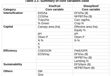
A summary of the slightly different core variables for the kiwifruit and sheep/beef analyses are shown in Table 2.1.

Table 2.1: Summary of core variables used

Kiwifruit Sheep/beef

Category Core variable Core variable

Intensification E0S/ha EFS/ha ($)

COS/ha NFPBT/ha ($)

Trays/ha Carc wgt/ha

% Green Crop %

Capital Canopy area (ha) Effective area (ha)

Equity %

pH pH

Olsen P Olsen P

N % N %

K S

Efficiency COE/GOR FWE/GFR

EOS/tray EFS/su ($)

NFPBT/su ($) Lambing %

Sustainability EFS/farm ($)

NFPBT/farm ($)

Others DM

Size

2.6 Method of analysis

1. Calculation of averages, trends (annual change), and variability

(17)

2. PCA

Separate Principal Components analyses were carried out for each set of variables – averages, trends and variation.

A Principal Components Analysis (PCA) reduces a data set of variables to a lesser number of independent variables which explain most of the variation. This is done by combining variables that are measuring the ‘same’ thing – that is, they are correlated. If these combined variables are easily interpreted, that is it they can be logically connected, the complexity of an analysis which would have otherwise had many more variables is reduced.

3. Cluster analysis

Cluster analyses were performed on the principal component scores for each analysis. A cluster analysis does the same as a PCA but for the units that make up a variable, in this case the measurements associated with each farm or orchard. Hence from this analysis we obtain groups of farms or orchards that have similar measurements on each Principal Component (PC).

4. Determining the cluster group characteristics

Unbalanced anova analyses were carried out on the original data using the groups determined by the cluster analysis. This showed how these groups played out in real values in the original data, to understand the implications in ‘real’ life of this grouping (rather than using the combined Principal Component scores which do not have clear meaning).

One issue here was that some of the averages of the financial variables were not significantly different from zero as some orchards suffered losses rather than profits over the years for which this data was collected. As each cluster group average was only calculated for the data in its group any test of whether it was significantly different from zero only involved the variation of the data in that particular group (which may have only had 2 or 3 members) it meant the boundaries of the mean were often very wide because only a few degrees of freedom were involved. An alternative would have been to calculate the overall standard deviation and use that as an estimate of the s.d. of individual clusters/groups but no stats programme appears to do this and there have been so many analyses it would have been to labour intensive to do by hand! As a result in the tables the means that are not significantly different from zero have been bracketed, and are still taken account of in the commentary but less emphasis is placed on them.

5. Finding out how these groups differ in other on and off orchard/farm characteristics

The other collected variables were then analysed across the groups using unbalanced anovas. For the kiwifruit analysis this included eight further financial variables, eight further soil variables, four bird density variables and 100 attitude variables. For the sheep/beef this data included 14 further financial variables, four farm management variables, 21 fertiliser applications, three further soil variables and 100 attitude variables. This number of variables can then be multiplied by three because the mean, annual change and standard deviation (variability) was used for each variable. In addition of course, these variables had been in turn calculated from at least two years and up to 10 years of data.

2.7 Leaving out an outlier in sheep/beef

(18)

variation in lambing percentage. The transport costs were exceptionally high because of where the farm was located and that was compounded with the fact that the farmer was trading in stock. Perhaps this farm business is a lesson that farming also happens in a geographical context which has implications beyond the weather and physical attributes of the land.

2.8 Reading the tables

This report is full of a lot of dense information in tables as this is the most concise way of presenting a lot of information. The tables have been placed in two Appendices at the end of this report – Appendix 1 for the kiwifruit results and Appendix 2 for the sheep/beef results.

1. The tables use Duncan’s Notation to indicate significant differences between groups. The lower case letters placed as suffixes above means presented in the table indicate whether group means are significantly different at a 5 percent level, if they do not have a suffix in common. If these suffixes are bracketed it means there is a difference at a 10% level of significance.

2. This analysis uses least significant differences (lsds), the equivalent of t-tests. Some would argue that account needs to be taken of the fact that these analyses have used hundreds if not thousands of significance tests over hundreds of variables, and so it would be expected that at least 5% would show significance anyway, as a matter of chance. Account has not been taken of this. The author has choosen instead to make overall sense of the results, so that if one does not fit with what else appears to be happening, it has not been commented on as of importance.

3. Many numbers in the tables are bracketed. This has been used to indicate that this number is not significantly different from zero – that is, the 95% confidence interval for this mean included zero. So, for instance if measuring profit, and the mean is bracketed, it cannot be stated that it is likely that this group is making a profit. If it is an annual trend mean that is bracketed then it can be stated that it is unlikely that there is an average change over time occurring for this group. Similarly, if it is an average of standard deviations (s.d.) as a measure of variability or consistency over time that is bracketed, then it can be stated that it is likely this group has had a consistent level of profit from year to year. However, some of these non-significant means can then be declared to be significantly different by the analysis. This comes about probably because the calculation of the standard error of the differences, and hence the lsd, is a tighter analysis using all the available degrees of freedom for the full data set, whereas the calculation of the confidence interval for a single group mean probably has used only the data used to find that mean. For example, some of the groups have only two members, and the confidence interval for the group mean was calculated using (group mean ± t1 s.d./√2) where the s.d. is just calculated from the two data points, whereas testing the difference between two means used an lsd calculated from all 24 data points (if sheep/beef) or 29 if kiwifruit.

(19)

5. The p-value in the last column represents the probability, taken from the anova, of whether the factor group is statistically significant overall, i.e., is there an overall difference between the groups decided by the cluster analysis. Sometimes an individual difference has been found between two groups even though there is not an indication of an overall difference.5

The next two chapters report on the results of the kiwifruit and the sheep/beef analyses.

5

(20)

3 Results of Kiwifruit Analysis

3.1 Correlations

3.1.1 Correlation of averages

The table from which the following comments are drawn is Table 3.1 which can be found in Appendix 1. It appears that for kiwifruit the canopy area is strongly reflected in the financial statistics – that is the orchard size affects the financial efficiency of an orchard – the larger the orchard, the greater its profit (EOS/ha, COS/ha, EOS/tray) is likely to be, and the lower the EOS/GOR ratio. This is also reflected in the other financial statistics such as the greater the profit, the lower the EOS/GOR ratio.

It is reassuring to see obvious things reflected in this data, such as the average number of trays of fruit produced per ha is related to the average size of fruit produced – the larger the fruit ( the more trays/ha, as would be expected. Also, as we know, gold vines produce more fruit per ha, have a higher DM on average and are usually larger, and this is reflected here, i.e., the proportion of an orchard that is green is negatively related to the average number of trays/ha and the DM but positively related to fruit count size. In other words, as the proportion of Gold increased, the number of trays, dry matter and fruit size all increased.

In terms of the soil measurements it would appear that the percentage of N and the soil K are positively correlated and that soil K also correlates with the pH. The soil S measure also correlated with N% and soil K. Annually, orchardists typically apply combinations of fertiliser products with the aim of supplying these nutrients so these results are not surprising.

More intriguing is how COE/GFR correlates negatively with pH and positively with soil S. That is the less that is spent as a proportion of revenue the higher the pH.6 It would seem that a higher soil S costs an orchard. This is also reflected in the greater the COS the lower the soil S, which could be an indication of the cost of S fertiliser.

It is also intriguing that DM is negatively correlated with fruit count size meaning that the bigger the fruit the higher the DM. The opposite might be expected given that larger fruit might be expected to contain more water due to practices such as the use of N fertiliser.

Fruit DM is negatively correlated with soil pH, which could indicate that DM increases with a lower availability of soil nutrients. However, DM is not correlated with orchard returns, which could have been expected as a premium is paid for high DM fruit.

3.1.2 Correlation of change over time

When looking at the changes orchardists have made over the time (Appendix 1,Table 3.2) of the collection of this data (9 years for financial data, 10 years for production data and 3 years for soil data) it can be seen that lifting DM correlates with lowering profitability and production, and increasing the COE/GOR ratio. The first and last two issues are confounded with the dropping value of kiwifruit over the past few years, whereas the changing production probably reflects that the increased payment for DM means that orchards have focused less on production in order to increase their DM content. It implies that producing higher DM may have either increased an orchard’s working expenses or decreased GOR, or both.

6

(21)

Changes in the financial statistics are reflected in the correlations between these variables and their links to changes in production. Increasing production also results in a lowering of the COE/GOR ratio, indicating increased efficiency.

Keeping in mind that the soil measurements of annual change are only based on 3 years of data (2004, 2006 and 2009) an increase in pH is related to a reduction in the COE/GOR ratio,

indicating increased efficiency. This result is also a dilemma and possibly related to changing the DM as indicated above, i.e., is the increase in pH due to lower inputs of fertilisers that would otherwise lower pH? Increasing soil K is correlated with a decreasing DM. This is also a curious result as it is known that KF make a heavy drain on soil potassium.

3.1.3 Variability over time

As would be expected variability in one financial measure is reflected in the variability of other financial measures (see Table 3.3). The variability in production is related to the variability of fruit size, but what is surprising is that this does not seem to reflect on the variability of the profitability or the efficiency of the orchard’s financial arrangements, which probably indicates some smoothing capacity of the orchardist to maintain financial consistency.

A varying Olsen P measurement is reflected in the variation of soil N, and in a varying DM. A varying DM reflects in the variability of the profit made per tray (EOS/tray) but not on other financial measures.

3.2 Analysis of averages of kiwifruit data

3.2.1 Overall changes over the years of ARGOS

Before analysing the data into groups it is useful to examine the context in which kiwifruit growers have found themselves over the past 8 years and to consider overall responses to that context. The ZESPRI annual report for the year ended 2011 notes that the 2009/10 year was a challenging one and that uncertainty will continue with the psa incursion and the continuing volatility of the exchange rate (ZESPRI, 2011). Figures in the annual report (pp.3-4) show the variability of orchard gate returns (per tray and per ha) with the rather extraordinary increases in payments for Gold fruit eclipsing the more stable but much lower payments for Organic Green and Green fruit in the last two years. (In contrast the ARGOS data is adjusted so that prices are based on those in the year 2009 so that they are more comparable and if ZESPRI had done this the prices returned to orchardists would probably show a decline.)

The following analyses (see Table 3.4), like those that follow it, make no distinction between green, organic green and gold kiwifruit orchards. The next table shows the overall average annual change in the variables is analysed in more detail later. Gross Orchard Return/ha (GOR/ha) is the only measure which incorporates returns from the market over which orchardists do not have any control, however, orchardists do of course, have a certain amount of control over how much they produce to send to the market. All other variables can be seen as partial responses to the global market context in which orchardists find themselves. (Other things over which orchardists have no control are the type of base soil resource of their orchard, the weather and other associated climate variables. It is proposed that classifications be studied as part of ARGOS 2.2.) Some components of orchard working expenses such as fuel, sprays and chemicals will be associated with externally driven, rising prices, but this is confounded by the choice orchardists make with regard to how much of these products they use.

(22)

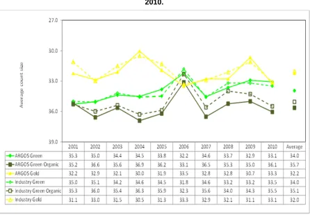
is adjusted to take account of expenses to get a measure of the profit, EOS/ha has not changed for Green and Gold orchards but has dropped for Organic Green. When profit is measured by COS/ha both Green and Organic Green have experienced a drop in profit. At the same time the overall production (trays/ha) has increased, indicating a major response to falling profits is to increase production – to intensify. This is partly indicated by the decrease in the return per tray (EOS/tray) for Organic Green. Over this period the overall soil resource has increased with increases in pH, Olsen P, N % and K. At times this is revealed partly as a result of the increased power of the larger sample size when all 29 orchards are included in the analysis. The only measured element that has not increased is K for Organic Green orchards. This is because it is difficult for organic orchardists to find a good source of K that complies with organic standards. The efficiency of the orchard operation has not changed significantly over the period for all orchards but when organic were considered separately their efficiency had actually become slightly worse. Organic orchardists had actually increased their DM % over the period but the Gold orchardists dropped theirs. The later trend is largely a consequence of high DM early on when the Gold plants were not yet fully mature (See Figure 1). Overall there was no change in size or DM.

Figure 3.1: Average count size of export fruit from ARGOS and industry orchards 2001- 2010.

Source: Jayson Benge.

(23)

orchardists used less), it is apparent that Organic Green orchardists cut their spray and chemical costs, while Green orchardists increased their fertiliser costs. (Analyses of results according to management system are reported in greater detail and are available on the ARGOS website.)

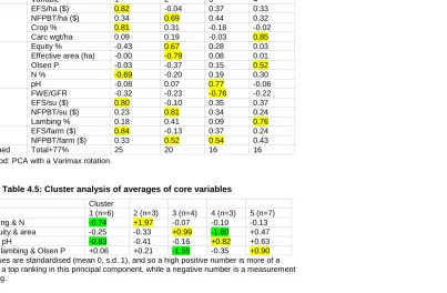
3.2.2 PCA analysis of averages of core variables

For the first analysis (of averages) the data reduced to four Principal Components (Table 3.5) so each orchard in the data set was assigned a score on each of these PCs. In the table the highlighted cells indicate the variables that are a major influence on each principal component. It can be seen that the first principal component, PC1, measures profit and efficiency of production in financial terms, with canopy area now being seen to be associated with financial efficiency. In contrast PC2 measures production, with a negative association with whether an orchard is mainly producing green or gold fruit, a positive emphasis on DM and larger fruit. The third component measures the soil resource except for pH, and the fourth the soil resource associated with pH and soil K. This seems a very satisfactory allocation, easily interpreted across the variables.

3.2.3 Cluster analysis of averages of core variables

A cluster analysis carried out on the four PCs of the 14 averages of the core variables for each orchard (Table 3.6). The 5 cluster solution was chosen because it separated the orchardists into more contrasting and interesting groups. The following descriptions of the groups formed by the cluster analysis are obtained from anovas carried out firstly, on the original core variables from which the PC scores were formed (Table 3.7), secondly on the annual change (Table 3.8) and variation of the core variables (Table 3.9), thirdly, on the other financial and orchard management variables we have collected (Table 3.10), fourthly on the bird intensities calculated from three different periods of observation and counts made on birds on the orchards (Table 3.11), and finally on the attitude data obtained from a survey carried out in 2008 (Table 3.12). The tables summarising the full results of this data can be found in Appendix 1.

Group 1 – poor production, challenging environment

Members: 1A, 5A (2 green)7

The measures of the PCs (Table 3.6) indicate that this group has lower productivity and the lowest soil resource in terms of pH and K, compared with the others. Accordingly, looking at the analysis of the averages of the core variables in the PCA (Table 3.7), Group 1 has one of the lower COS/ha, is the most acidic (lowest pH) and has a lower K soil measurement. It has the greatest average canopy area. Both these orchards are in challenging locations – Kerikeri and at a higher altitude in the Bay of Plenty. However, the matching gold orchard (5C, Group 4) is doing very well, but the matching organic orchard (5B, Group 3) is also struggling, possibly due to the high altitude environment, but it is in Group 3 because it has a high soil resource. Group 1 also has one of the more variable COS/ha which is reflected in the high variability of the production (trays/ha) (see Table 3.9).

Group 1 has the lowest expenditure on electricity and fertiliser, and the highest expenditure on pollination (which may be due to location). This group has the lowest density of introduced insectivorous birds which also may be a location effect.

In terms of attitudes this group is one of those that places a high importance on things associated with biodiversity and environmental wellbeing – soil biological activity, having a diversity of native birds, plants and trees, taking responsibility for encouraging birds, enhancing

7

(24)

stream health with trees and shrubs. The two orchardists in this group were most supportive of using trees to make their orchards look attractive and they expect to be orcharding for a long time.8 They have no debt.

Group 2 - low performing, inefficient, inconsistent and poor soil resource

Members 1C, 6A, 6C, 7A, 7C, 8C, 11A, 11B (3 green, 1 organic green, 4 gold) 9

According to the cluster analysis this group should have the lowest financial averages in terms of both profit and efficiency, the least soil resource in terms of N%, Olsen P, K and S, and the smallest orchards. The analysis of core variables indicated that indeed Group 2 made on average, the greatest loss per hectare and was the least efficient (highest COE/GFR, greatest loss for each tray of fruit produced), it had the least canopy area, lower N% and K but the highest Olsen P measurement.10 The lower soil nitrogen appears to be recognised by the orchardists in this Group 2 because this group also has the highest application of N fertiliser.

When considering the trend and variation variables (Tables 3.8 and 3.9), Group 2 had the least change (and the lowest variation) in the soil percentage of N, but the greatest variation in production, efficiency, fruit size and in the amount of S fertiliser applied11. This demonstrates that they consistently apply the same amount of N fertiliser each year but that many other factors influence their production and returns.

We know that Cluster 11 (2 orchards in this group) was badly affected by frost in the early years of ARGOS and this may have contributed to the large variation seen in production and fruit size.

Group 3 - high soil resource not matched by financial return and production

Members 2A, 2C, 3A, 3B, 4A, 4B, 4C, 5 B (3 green, 3 organic green, 2 gold)

The cluster analysis indicates that Group 3 should have the highest soil resource. Looking at the analysis of the core variables Group 3 does have the highest pH, N, K and S soil measurements. The pH is actually higher than that recommended for kiwifruit (Hill Laboratories (2) & (3), n.d.), but the N and K readings are within the recommended medium range. The S reading is regarded as high. This group has the lowest Olsen P measurement, just making it within the recommended range of 30 to 60. It has lower profit and production figures, and these are supported by a lower DM average.12 Group 3 orchards are also smaller.

From the analysis of the change and variability variables (Tables 3.8 and 3.9), it can be seen that Group 3 shows the greatest increase in N% and the greatest variability in N% and pH - one probably leading to the other. Group 3 has been lifting its N%, over the time period in which the

8

Ironically, one of these orchardists has sold his orchard since this survey was carried out in 2008.

9

One of the orchards in this group could be considered an unusual one to have here because it has been regarded as an exemplar for high production. However, although it is a high producer, our figures show that the soil resource of this orchard is by far the lowest in the group, and that over all the years that ARGOS has been collecting data the applications of all fertilisers (except Mg) have been dropping. Maybe, as this orchardist has looked towards retirement he has been reducing his costs.

10

All Olsen P group averages are in the medium range (30 – 80) and this is the highest within that. It could be because this group has the smallest proportion of organic orchards and organic orchards usually have a lower Olsen P (Carey et al., 2009).

11

Variation can presumably come about because of weather events or changes made in orchard practices that may or may not result in consistent change.

12

(25)

measurements were taken (2004, 2006, 2009),13 and as shown in the former table, it has the highest average levels of this soil measurement. This change does not appear to be associated with changes in production or financial returns. It has some of the most consistent COS/ha, GOR/ha and efficiency measures as calculated by COE/GOR but as the COS/ha and GOR/ha are low and the efficiency is high (i.e., less efficient) this is not good news because it implies that the practices inbuilt to produce these results are unlikely to change.

Group 3 has the highest phosphate application, and the variation in sulphur application is also high. It ranks highly for all electricity expenses (average, increase and variability), for spray and chemicals costs (average and variability) and fertiliser costs (average and variability), and it has a high variation in pollination costs. Though it has the greatest annual drop in orchard working expenses (OWE/ha), these overall expenses are also very variable. Therefore, it can be seen that this group contribute to building the soil resource, and are working to reduce expenses, but are still not making a profit.

In terms of attitudes, this group consist of ‘the pleasers’- it consistently has the highest score for any of the variables which show a difference across any of the groups. The orchardists in this group place importance on environmental and social indicators, they are less likely to change or promote diversity of income sources and are not sure about birds on the orchard, but do see it as landowners' responsibility to encourage birds, they are supporters of planting native trees and have low debt.

The high level of importance and agreement placed on all these variables perhaps indicates that this group like to be thought well of and to socially conform.

Group 4 - the highest producers, spenders and profit makers

Members 3C, 5 C, 9C (3 gold)

The cluster analysis suggests that Group 4 should have the highest profit and productivity and be very efficient. The analysis of the core variables indicates that this is so. Group 4 made the most profit (EOS/ha14, COS/ha, EOS/tray) and produced the most trays/ha, with the highest DM and the largest fruit. Their COS/ha and pH were the most variable. The soil measurements indicate that these orchards fall within the medium recommended ranges for their soil resource.

Group 4 had the highest Gross Orchard Return (GOR/ha), spent more on sprays and chemicals and fertiliser, which contributed to the highest working expenses (COE/ha). However, the group’s GOR/ha is the most variable as are their working expenses which are also the most changeable and possibly increasing. This group is maintaining expenditure on electricity. The members of this group are prepared to spend a lot on their orchard but manage to do it in such a way that they make a good return, however, this is averaged over several years, rather than being consistent. In terms of attitudes this group is not concerned about what people think of them. In the survey they claim that environmental values and biodiversity are not important to them and they do not see the orchard as contributing to the environment. (This is a curious aspect of this because we know that one of the orchards is owned by a couple with strong environmental values. However, we know that in the survey they scored anything to do with biodiversity lower than many of the others.) This probably indicates that this group consists of high input orchardists who can make high profits but this is variable possibly because they are

13

However, the soil results are only based on three measurements and so not too much emphasis should be placed on them.

14

(26)

trying things out all the time, taking risks and constantly changing. A high variability can imply adaptability and year to year management, rather than doing the same thing year after year.

Note that these results could just be attributable to these group members all being gold producers as gold fruit naturally has higher DM than green fruit, is a larger producer and has larger fruit, but this study is about pathways to sustainability so is this result saying that given the choice,15 it would be good idea to produce gold fruit.16 However, we have to point out that there are nine gold orchards in this data analysis and only three appear in this clustering indicating that the success of Gold is also dependent on the orchardist, management and the site. The next grouping challenges the sustainability of this group.

Group 5 – most efficient, consistent and profitable

Members 6B, 7B, 8B, 9A, 9B, 10A, 10B, 12B (2 green, 6 organic green)

The cluster analysis indicated that this group was making the highest profit, being the most efficient and as having the lowest level of production. The analysis of the core variables indicates that this is so with Group 5 making the most profit (EOS/ha, COS/ha) (alongside Group 4), being the most efficient (lowest COE/GOR, highest EOS/tray) and producing the least trays/ha. However, it also has the lowest average DM and grows the smallest fruit from a lower soil resource in terms of N%, K and S. The pH is higher than recommended (Hill Laboratories (1) and (2), n.d.). The orchards are larger on average than those of Groups 2 and 3.

The analysis of the variability of the core variables indicates that Group 5 has the most consistent and reliable production, fruit size, efficiency and soil pH.

The GOR/ha for the orchards in Group 5 is not higher than that for Groups 2 and 3 which are possibly making a loss, so how is it this group is making a stable profit (COS/ha) over the years of ARGOS? An examination of 'other' variables reveals that this group has the least variation in COE/ha. This is because it is among the groups with the least variation in expenses associated with electricity, spray and chemicals, pollination and fertiliser, but it is the sole group with low variation in all these expenses. The group average is lower for expenditure on spray and chemicals, pollination and fertiliser and together this contributes to the lowest COE/ha overall. The considerably lower expenditure on pollination and spray and chemicals contributes most to this result (and the low expenditure on spray and chemicals could well be because a greater proportion of the orchards in group 5 are organic). All of these results indicate a low intensity production system and this lack of intensification may well be indicated by the highest density of introduced insectivorous birds. The members of this group are the least concerned about issues to do with the family and succession. They are bird friendly but not tree friendly. They focus on a limited number of income sources, probably only growing green kiwifruit, seldom deviate from plans, and do not see their orchard as changing much over the next ten years. This suggests, when taken alongside the low variation in most variables, that the orchardists in this group are probably doing what they have always done and are probably not very adaptable. They probably are looking towards retirement though there was no indication that they were any older than orchardists in the other groups.

One of the orchards in this group - 6B - is the biggest in ARGOS. The members of this group are also mainly based around Te Puke which may result in some sort of efficiency advantage.

15

The licences to grow Gold fruit are limited.

16