Statistical Methods for Compositional and Tree-Structured Count Data in Human Microbiome Studies

(1)

University of Pennsylvania

ScholarlyCommons

Publicly Accessible Penn Dissertations

1-1-2016

Statistical Methods for Compositional and

Tree-Structured Count Data in Human Microbiome

Studies

Pixu Shi

University of Pennsylvania, [email protected]

Follow this and additional works at:

http://repository.upenn.edu/edissertations

Part of the

Biostatistics Commons

This paper is posted at ScholarlyCommons.http://repository.upenn.edu/edissertations/2013 For more information, please [email protected].

Recommended Citation

Shi, Pixu, "Statistical Methods for Compositional and Tree-Structured Count Data in Human Microbiome Studies" (2016).Publicly Accessible Penn Dissertations. 2013.

(2)

Statistical Methods for Compositional and Tree-Structured Count Data in

Human Microbiome Studies

Abstract

In human microbiome studies, sequencing reads data are often summarized as counts of bacterial taxa at

various taxonomic levels. In this thesis, we develop statistical methods for analyzing such counts data. We first

consider regression analysis with bacterial counts normalized into compositions as covariates. In order to

satisfy the subcompositional coherence of the resulting model, linear models with a set of linear constraints

on the regression coefficients are introduced. A penalized estimation procedure for estimating the regression

coefficients and for selecting variables under the linear constraints is developed. A method is also proposed to

obtain de-biased estimates of the regression coefficients that are asymptotically unbiased and have a joint

asymptotic multivariate normal distribution. This provides valid confidence intervals of the regression

coefficients and can be used to obtain the p-values. Simulation results have shown the validity of the

confidence intervals and smaller variances of the de-biased estimates when the linear constraints are imposed.

The proposed methods are applied to a gut microbiome data set and identify four bacterial genera that are

associated with the body mass index after adjusting for the total fat and caloric intakes.

We then consider the problem of testing difference between two repeated measurements of microbiome from

the same subjects. Multiple microbiome measurements are often obtained from the same subject to assess the

difference in microbial composition across body sites or time points. Existing models for analyzing such data

are limited in modeling the covariance structure of the counts and in handling paired multinomial data. We

propose a new probability distribution for paired multinomial count data, which allows flexible covariance

structure of the counts and can be used to model repeatedly measured multivariate counts. Based on this new

distribution, a test statistic is developed to test the difference in compositions of paired multinomial count

data. The proposed test can be applied to count data observed on taxonomic trees in order to test difference in

microbiome compositions and to identify subtrees with different subcompositions. Simulation results shown

that the proposed test has correct type 1 errors and increased power compared to some commonly used

methods. An analysis of an upper respiratory tract microbiome data set is used to illustrate the proposed

methods.

Degree Type

Dissertation

Degree Name

Doctor of Philosophy (PhD)

Graduate Group

Epidemiology & Biostatistics

First Advisor

(3)

Keywords

compositional data, high-dimensional regression, hypothesis testing, microbiome, paired count data,

taxonomic tree

Subject Categories

(4)

STATISTICAL METHODS FOR COMPOSITIONAL AND TREE-STRUCTURED COUNT DATA IN HUMAN MICROBIOME STUDIES

Pixu Shi

A DISSERTATION

in

Epidemiology and Biostatistics

Presented to the Faculties of the University of Pennsylvania

in

Partial Fulfillment of the Requirements for the

Degree of Doctor of Philosophy

2016

Supervisor of Dissertation

Hongzhe Li, Professor of Biostatistics

Graduate Group Chairperson

John H. Holmes, Professor of Medical Informatics in Epidemiology

Dissertation Committee

Nandita Mitra, Associate Professor of Biostatistics

Frederic D. Bushman, William Maul Measey Professor in Microbiology

T. Tony Cai, Dorothy Silberberg Professor in Statistics

(5)

ACKNOWLEDGEMENT

I would like to thank my advisor Dr. Hongzhe Li, who has been an extraodinary mentor during the

past four years. His expertise, vision and perspicacity in the field make it possible for me to work

on such an exciting and promising research topic. My life as a PhD student has been very smooth

given his kindness, generosity and constant support. I feel very fortunate to start my career working

with Dr. Li.

I would like to thank my committee chair Dr. Nandita Mitra for watching over me in every step from

matriculation to graduation. Her upbeat and warm personality makes it a delightful experience to

work with her. I am also very grateful to my committee members Dr. Rick Bushman, Dr. Tony Cai

and Dr. James Lewis for providing valuable comments and encouragements.

I would like to express my gratitude to my coauthors Dr. Wei Lin, Dr. Dylan Small, Colin Fogarty

and my fellow student Eric Zhang Chen for their help in my research. I am also thankful for having

the joyful company of my friends from Penn Biostatistics.

Last of all, I would like to thank my husband Anru Zhang for being supportive in every aspect of

my life. He bears with my crankiness when I have difficulties and brings fresh views to my work by

(6)

ABSTRACT

STATISTICAL METHODS FOR COMPOSITIONAL AND TREE-STRUCTURED COUNT DATA IN

HUMAN MICROBIOME STUDIES

Pixu Shi

Hongzhe Li, PhD

In human microbiome studies, sequencing reads data are often summarized as counts of bacterial

taxa at various taxonomic levels. In this thesis, we develop statistical methods for analyzing such

counts data. We first consider regression analysis with bacterial counts normalized into

composi-tions as covariates. In order to satisfy the subcompositional coherence of the resulting model, linear

models with a set of linear constraints on the regression coefficients are introduced. A penalized

estimation procedure for estimating the regression coefficients and for selecting variables under

the linear constraints is developed. A method is also proposed to obtain de-biased estimates of the

regression coefficients that are asymptotically unbiased and have a joint asymptotic multivariate

normal distribution. This provides valid confidence intervals of the regression coefficients and can

be used to obtain the p-values. Simulation results have shown the validity of the confidence

in-tervals and smaller variances of the de-biased estimates when the linear constraints are imposed.

The proposed methods are applied to a gut microbiome data set and identify four bacterial genera

that are associated with the body mass index after adjusting for the total fat and caloric intakes.

We then consider the problem of testing difference between two repeated measurements of

mi-crobiome from the same subjects. Multiple mimi-crobiome measurements are often obtained from the

same subject to assess the difference in microbial composition across body sites or time points.

Ex-isting models for analyzing such data are limited in modeling the covariance structure of the counts

and in handling paired multinomial data. We propose a new probability distribution for paired

multi-nomial count data, which allows flexible covariance structure of the counts and can be used to

model repeatedly measured multivariate counts. Based on this new distribution, a test statistic is

developed to test the difference in compositions of paired multinomial count data. The proposed

test can be applied to count data observed on taxonomic trees in order to test difference in

(7)

shown that the proposed test has correct type 1 errors and increased power compared to some

commonly used methods. An analysis of an upper respiratory tract microbiome data set is used to

(8)

LIST OF TABLES

TABLE 2.1 : Means and standard errors (in parentheses) of various performance mea-sures for three methods based on 100 simulations . . . 16 TABLE 2.2 : Selection probabilities and refitted coefficients of four selected genera in the

gut microbiome data . . . 19

TABLE 3.1 : True/False positive rates of the significant variables selected based on95% confidence intervals constructed using multiple, one and no linear constraints, labeled by ‘Multi’, ‘One’ and ‘No’ respectively. Variable correlationsζ, num-bers of variablespand sample sizes (n) are considered. . . 39 TABLE 3.2 : Testing set prediction error of the LASSO estimator, refitted estimator with

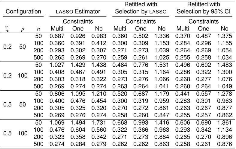
variables selected by byLASSO, and refitted estimator with variables select-ed basselect-ed on95% confidence intervals. For each estimator, model was fit using multiple, one and no linear constraints. Variable correlationsζ, num-bers of variablespand sample sizes (n) are considered. . . 40

TABLE 4.1 : p−values of different comparisons between two body sites and between

(11)

LIST OF ILLUSTRATIONS

FIGURE 2.1 : Analysis of gut microbiome data. (a) Selection probabilities with boot-strapped crossvalidation for 87 genera that belong to eight phyla. Selec-tions with a positive sign and a negative sign are shown by dark grey blocks and light grey blocks, respectively; only four major phyla are indicated. (b) Fitted versus observed values ofBMI. . . 18

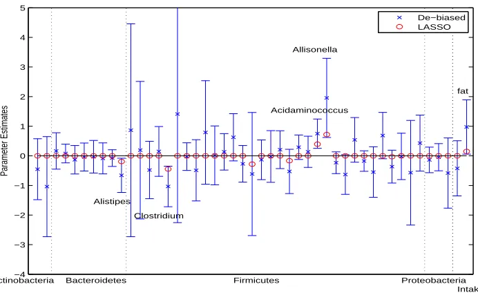
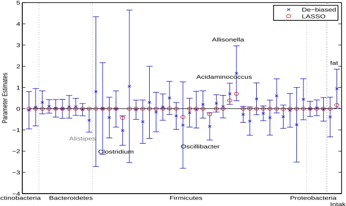
FIGURE 3.1 : Analysis of gut microbiome data. Lasso estimates, de-biased estimates and 95% confidence intervals of the regression coefficients in the model treating the composition of 45 genera as covariates together with total fat and caloric intakes. Dashed vertical lines separate bacterial genus into different phyla. . . 34 FIGURE 3.2 : Analysis of gut microbiome data. Lasso estimates, de-biased estimates

and 95% confidence intervals of the regression coefficients in the model treating the subcompositions of the genera in each phylum as covariates together with total fat and caloric intakes. Dashed vertical lines separate bacterial genus into different phyla. . . 35 FIGURE 3.3 : Analysis of gut microbiome data. Observed and predictedBMIusing LOOCV

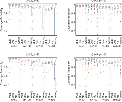
and variables selected based on 95% confidence intervals, together with total fat and caloric intakes. . . 36 FIGURE 3.4 : Coverage probabilities of confidence intervals based on 100 replications.

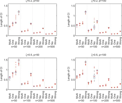
For each model, minimum, median (in red line), mean (in red dot) and maximum of the coverage probabilities over compositional covariates are shown. The confidence intervals are constructed using multiple, one, no and wrong linear constraints, labeled by ‘Multi’, ‘One’, ‘No’ and ‘Wrong’ respectively. . . 37 FIGURE 3.5 : Average lengths of confidence intervals based on 100 replications. For

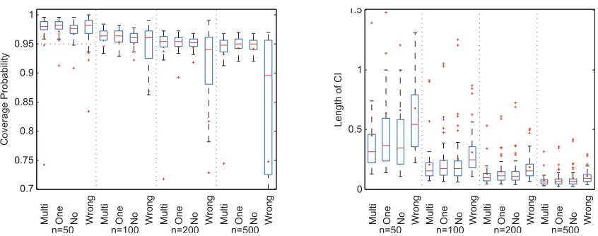
each model, minimum, median (in red line), mean (in red dot) and maxi-mum of the lengths of the intervals overall all compositional covariates are shown. The confidence intervals are constructed using multiple, one, no and wrong linear constraints, labeled by ‘Multi’, ‘One’, ‘No’ and ‘Wrong’ respectively. . . 38 FIGURE 3.6 : Coverage probabilities and length of confidence intervals based on 500

replications. Data are simulated by resampling the gut microbiome compo-sition data in Section 3.5. . . 41

FIGURE 4.1 : Simulation results: size and power of the paired and unpaired tests for data simulated under the PairMN model (a) and the correlated log-normal model (b) for sample sizen=20,50and 100. x-axis is the correlation parameterρ. 58 FIGURE 4.2 : Taxonomic tree of the gut microbiome samples from which the simulated

data are generated. In our simulations, the count of genus Streptococcus is perturbed to generate samples from the alternative distribution. . . 59 FIGURE 4.3 : Comparison of rejection rate of the proposed method with PERMANOVA

with the level of test atα=0.05. X-axis is the perturbation percentage pε,

(12)

FIGURE 4.4 : Identification of subtrees with differential subcompositions with FDR set to 0.05. Y-axis shows the percent of discovery of the corresponding subtree in 100 simulations with FDR controlled at 0.05. The empirical FDR is close to 0.05. . . 60 FIGURE 4.5 : Parental nodes and the child nodes that showed differential

subcomposi-tion between nasopharynx and oropharynx. . . 61 FIGURE 4.6 : Parental nodes and the child nodes that showed differential

(13)

CHAPTER 1 I

NTRODUCTION

1.1. Human microbiome and human health

A typical human body is inhabited by at least 10-100 trillion microbes, outnumbering the human

cells by an estimated 10-fold (Turnbaugh et al., 2007). The community formed by microbes,

mi-crobiota, includes bacteria, fungi, archaea and viruses, and can be found at various human body

sites such as gut, skin, oral cavity, vagina, respiratory tract,etc.. The collective genome of human

microbiota, also known as thehuman microbiome, is estimated to contain∼150 times more genes

than the human genome (Qin et al., 2010). Compared with the human genome, the human

micro-biome has much more diversity. The microbiota found at different body sites of the same individual

can differ remarkably, and even at the same body site, human microbiome can display substantial

inter-individual variation (Consortium et al., 2012) and temporal variation within the same individual

(Flores et al., 2014; Grice et al., 2009).

Many recenyt studies have been investigating the role of microbiome in human health. For

exam-ple, the gut microbiome has been shown to be associated with many human diseases such as

obesity, diabetes and inflammatory bowel disease (Ley et al., 2005, 2006; Manichanh et al., 2012;

Qin et al., 2012; Turnbaugh et al., 2006); the skin microbiome has been postulated to have

contri-bution to several skin disorders (Grice et al., 2009; Kong et al., 2012). The health and lifestyles of

host have also been shown to affect the composition of microbiome. Studies have found that

long-term dietary habits affect the composition of gut microbiota (Wu et al., 2011, 2014). The microbial

communities in the upper respiratory tract of cigarette smokers differ between smokers and

non-smokers (Charlson et al., 2010; Morris et al., 2013). The host genotypes also have influence on the

microbiota compositions (Spor, Koren, and Ley, 2011; Turnbaugh et al., 2006). These links between

human microbiome and human health indicate the possibility of designing therapeutic strategies for

treatment of complex diseases and conditions by modulating the microbial composition (Cani and

Delzenne, 2011; Hsiao et al., 2013; Smits et al., 2013; Virgin and Todd, 2011), and the potential of

using microbiome as biomarkers for disease prevention and early diagnostics (Gevers et al., 2014;

(14)

the Human Microbiome Project (HMP) (Peterson et al., 2009) and The European Union Project

on metagenomics of the human intestinal tract (MetaHIT) (Ehrlich, Consortium, et al., 2011) have

provided important data on human microbiome.

1.2. Investigating human microbiome through sequencing

To understand the impact of the human microbiome on human health, it is necessary to

character-ize and decipher the content of human microbiome. Prior to the invention of Sanger sequencing

technology in 1977 (Sanger, Nicklen, and Coulson, 1977), microbiota characterization largely relied

on culture-based methods, which are highly biased and time-consuming. The advent of Sanger

se-quencing allowed for some more thorough view of microbial communities, but is still limited in use

by its high cost and low throughput. With the development of next-generation sequencing

tech-nology such as Roche (454) pyrosequencing, Illumina Solexa sequencing and Applied Biosystems

SOLiD sequencing, researchers are now able to study the human microbiome with much lower cost

compared to older Sanger method, yet still achieve a coverage of microbial genes thorough enough

to characterize the true microbial population.

Two high-throughput sequencing based approaches have been used for interrogating complex

mi-crobial communities. The first approach is based on sequencing the 16S ribosomal RNA (rRNA)

amplicons. The 16S rRNA is a structural component of the prokaryotic ribosomes, and thus is

p-resented in all bacteria and archaea cells. The 16S rRNA gene contains highly conserved regions

that can be used as primer binding sites in PCR amplification, while its hypervariable regions can

be used to identify different bacterial lineages. After sequencing, the 16S sequences are clustered

into sequence clusters calledOperational Taxonomic Units (OTUs) using software pipelines such

as Qiime (Caporaso et al., 2010). The representative sequences of each OTU are then compared

to the existing 16S databases such as Greengenes (DeSantis et al., 2006), RDP (Cole et al., 2007)

and EzTaxon-e (Kim et al., 2012) to obtain taxonomic assignments. The ubiquitous presence of

16S rRNA enables lineage assignments at the levels of kingdom, phylum, class, order, family and

genus simultaneously.

Another approach is based on shotgun metagenomic sequencing, which sequences all the

micro-bial genomes presented in the sample, rather than just one marker gene. This approach enables

(15)

microorganisms such as viruses. The accuracy of this approach in quantifying gene/microbe

abun-dance is highly dependent on the DNA preparation protocols, which demands special cautions for

comparative metagenomic studies (Morgan, Darling, and Eisen, 2010). The massive amount of

short reads produced also requires efficient computational tools to perform read mapping and

as-sembly, which imposes more challenges in the applications of this approach. Several databases

and software tools have been developed to analyze the shotgun metagenomic data (Huson et al.,

2007; Meyer et al., 2008; Segata et al., 2012; Seshadri et al., 2007).

1.3. Data structure

1.3.1. Tree-structured count data on taxonomic tree

The taxonomic tree is a tree-structured diagram that illustrates the taxonomic classifications of

bi-ological organisms, with each tree node representing a taxon from the taxonomic rank of kingdom

to species. For 16S rRNA sequencing, since the same marker gene is used in taxonomic

assign-ments at all ranks, each read compared to the reference database can be subsequently aligned to

a node of the taxonomic tree depending on its taxonomic assignment. The resulting data is a set

oftree-structured count datawith each count number representing the number of reads aligned to

the corresponding node on the taxonomic tree.

This data format has several features: (1). The total number of reads varies greatly from sample to

sample. This can be attributed to the difference in sequencing depth and the amount of DNA

yield-ing materials. (2). The number of reads at each internal node is larger or equal to the sum of read

numbers at all its child nodes. This comes from the fact that if a read is assigned a certain taxon,

then all the higher ranked taxa along this lineage can also be assigned to this read. (3). There may

be a lot of zero counts, which can be caused by the rarity or absence of the corresponding bacteria.

The analysis of tree-structured count data is difficult due to high dimensionality, non-normality and

the tree structure underlying the data. Many of the current methods applied to this type of data have

been distance-based (Turnbaugh et al., 2006; Wu et al., 2011; Yatsunenko et al., 2012), where a

distance measure is defined and computed between each pair of the microbiome samples. One

commonly used distance measure is the UniFrac distance (Lozupone and Knight, 2005), upon

(16)

et al., 2012) and the phylogenetic Kantorovich–Rubinstein metric (Evans and Matsen, 2012). The

statistical methods based on these distance measures, such as Permutational multivariate analysis

of variance (PERMANOVA) (Anderson, 2001) and Principal Coordinate Anlaysis (PCoA) (Gower,

1966; Torgerson, 1958) are widely applied, their results are very dependent on the specific choice

of distance measure (Chen et al., 2012).

1.3.2. High-dimensional compositional data

Due to the varying number of reads across samples, the read counts from 16S rRNA sequencing

and shotgun metagenomic sequencing are often normalized into vectors of proportions at a given

taxonomic level. The resulting data are also referred to ascompositional data (Aitchison, 1982).

The unique feature that the components of a composition must sum to one renders many

stan-dard multivariate statistical methods inappropriate or inapplicable. Methodological developments

for compositional data analysis have resulted in a fruitful line of research, as thoroughly surveyed

by Aitchison (2003). While the dimensionality of compositional data from culture based microbial

analysis is often very small due to the limited number of cultivable bacteria, high-throughput

se-quencing technologies make it possible to identify hundreds of genera and species of bacteria

within one microbiome sample set. These large compositional data sets, whose dimensionality is

comparable to or much larger than the sample size, pose new challenges to existing

methodol-ogy. However, little formal attempt has been made to develop principled analysis tools for such

high-dimensional compositional data.

1.4. Organization of this thesis

My thesis focuses on the analysis of both high-dimensional compositional data and tree-structured

count data on taxonomic tree. In Chapter 21, we aim to address the variable selection problem in

regression analysis with high-dimensional compositional covariates. We propose an`1

regulariza-tion method for the estimaregulariza-tion and variable selecregulariza-tion in high-dimensional linear log-contrast model

that considers the unique features of the compositional data. We formulate the proposed

proce-dure as a constrained convex optimization problem and introduce a coordinate descent method

of multipliers for efficient computation. In the high-dimensional setting where the dimensionality

grows at most exponentially with the sample size, model selection consistency and`_∞bounds for

(17)

the resulting estimator are established under conditions that are mild and interpretable for

compo-sitional data. The numerical performance of our method is then evaluated by simulation studies

and its usefulness is illustrated by an application to a microbiome study relating body mass index

to human gut microbiome composition.

In Chapter 32, we consider the inference problem of high-dimensional regression analysis with

compositional data, where the goal is to identify the bacterial taxa that are associated with a

con-tinuous response such as the body mass index (BMI). In order to satisfy the subcompositional

coherence of the results, we propose to use linear models with a set of linear constraints on the

regression coefficients. Such models allow regression analysis for subcompositions and include

the log-contrast model for compositional covariates as a special case. An`1penalized estimation

procedure for estimating the regression coefficients and for selecting variables under the linear

con-straints is developed. To provide valid confidence intervals of the regression coefficients and obtain

the correspondingp-values, a method is proposed to obtain de-biased estimates of the regression

coefficients that are asymptotically unbiased and have a joint asymptotic multivariate normal

distri-bution. Simulation results show the validity of the confidence intervals and smaller variances of the

de-biased estimates when the linear constraints are imposed. The proposed methods are applied

to the same gut microbiome dataset as Chapter 2 and results are compared.

In Chapter 43_{, we consider the problem of testing difference between repeatedly measured}

micro-biome data quantified as counts on taxonomic tree. Such repeated data often occur when multiple

samples are taken from the same subject to assess the difference in microbial composition across

body sites or time points. To model the covariance structure of the count data with flexibility, we

propose a general class of probability distributions for paired multinomial count data, which allows

us to model repeatedly measured multivariate counts. Based on this new distribution, we develop a

test statistic to evaluate the difference in the mean parameters of paired multivariate count data. We

then provide a procedure that applies the proposed test to count data observed on an taxonomic

tree in order to assess difference in microbiome compositions and to identify subtrees with different

sub-compositions. Our simulation results indicate that proposed test has correct type 1 errors and

increased power compared to some commonly used methods. The proposed methods are

illus-trated by an analysis of the human pharynx microbiome data, where nasopharynx microbiome is

(18)

compared with oropharynx microbiome, and smokers microbiome is compared with non-smokers.

(19)

CHAPTER 2 V

ARIABLE SELECTION IN REGRESSION WITH COMPOSITIONAL COVARIATES

2.1. Introduction

Compositional data, which consist of the proportions or percentages of a composition, appear

frequently in a wide range of applications; examples include geochemical compositions of rocks

in geology, household patterns of expenditures in economics, species compositions of biological

communities in ecology, and topic compositions of documents in machine learning. The unique

feature that the components of a composition must sum to one renders many standard

multivari-ate statistical methods inapproprimultivari-ate or inapplicable. Since the seminal work of Aitchison (1982),

methodological developments for compositional data analysis have resulted in a fruitful line of

re-search, as thoroughly surveyed by Aitchison (2003). The recently increasing availability of large

compositional data sets, whose dimensionality is comparable to or much larger than the sample

size, poses new challenges to existing methodology. However, little formal attempt has been made

to develop principled analysis tools for such data. A typical example arises in metagenomic studies

of microbial communities based on 16S rRNA gene sequencing, where the relative abundances of

hundreds to thousands of bacterial taxa on a few tens to hundreds of individuals are available for

analysis; see, for example, Chen and Li (2013).

The aim of this chapter is to address the variable selection problem in high-dimensional

regres-sion with compositional covariates. To mitigate the difficulty with high dimenregres-sionality, it is crucial to

select parsimonious models that tend to improve the performance of statistical procedures and

in-terpretability of the resulting inferences. Regularization methods for simultaneous variable selection

and estimation in linear regression and more general contexts have received intense recent

inter-est. In particular, the`₁regularization or lasso approach (Tibshirani, 1996) has enjoyed widespread

popularity, and its theoretical properties in high-dimensional regression are now well understood;

see, for example, B ¨uhlmann and Van De Geer (2011) for an overview. Owing to the special nature

of compositional data, however, the usual linear regression model is inappropriate for our

purpos-es. In this chapter we consider the linear log-contrast model of Aitchison and Bacon-shone (1984),

(20)

the expected response does not depend on the basis counts from which a composition is obtained.

This is the case in our microbiome data example, where the number of sequencing reads varies

drastically across samples and should not play a role in predicting the response of interest.

We propose an`1regularization methodology for variable selection and estimation in high-dimensional

linear log-contrast models. We formulate the proposed procedure as a constrained convex

opti-mization problem, develop efficient algorithms for computation, and provide strong theoretical

guar-antees. Since the constraint in the problem couples the parameters, coordinate descent methods

for solving`1-regularized least squares problems (Friedman et al., 2007) are not directly applicable.

We therefore combine coordinate descent with the method of multipliers to introduce an efficient

algorithm for solving the optimization problem. To establish model selection consistency and `∞

bounds for the resulting estimator, we impose conditions analogous to the irrepresentability

condi-tion for linear regression in Zhao and Yu (2006). Our condicondi-tions, however, differ from those for linear

regression models in important ways, which account for the compositional effect and adapt well to

the dependence structure of compositional data.

2.2. Variable selection in the linear log-contrast model

Log-contrast models were originally introduced by Aitchison and Bacon-shone (1984) for modeling

experiments with mixtures, and have proved to be useful for a wide variety of regression problems

with a composition playing the role of covariate. Suppose that we observe ann-vectoryof

respons-es and ann×pmatrixX= (xi j)of covariates, with each row ofX lying in the(p−1)-dimensional

positive simplexSp−1={(x1, . . . ,xp): xj>0,j=1, . . . ,p,∑p_j₌₁xj=1}. Because of the unit-sum

con-straint, thepcomponents of a composition cannot vary freely, traditional methodology often requires

the omission of certain components to ensure identifiability and encounters intrinsic difficulties in

providing sensible interpretations for the regression parameters. To resolve the difficulties with the

compositional constraint, Aitchison and Bacon-shone (1984) proposed to apply the log-ratio

trans-formation (Aitchison, 1982) to compositional covariates, resulting in the linear log-contrast model

y=Zpβ_\∗_p+ε, (2.1)

whereZp={log(xi j/xip)}is then×(p−1)log-ratio matrix, whosepth component is the reference

(21)

ε is an n-vector of independent noise distributed as N(0,σ2). By introducing a new coefficient

β_p∗=−∑p_j₌−₁1β∗_j, model (2.1) can be more conveniently expressed in the symmetric form

y=Zβ∗+ε,

p

∑

j=1

β_j∗=0, (2.2)

whereZ= (z1, . . . ,zp) = (logxi j)is then×pdesign matrix andβ∗= (β₁∗, . . . ,βp∗)>is the p-vector of

regression coefficients. We do not include an intercept in the model, since it can be eliminated

by centering the response and predictor variables. We are concerned with the high-dimensional

sparse setting, where the dimensionalitypis comparable to or much larger than the sample sizen,

while only a small portion of the regression coefficients are nonzero.

Applying the `1regularization approach to model (2.2), we consider the constrained convex

opti-mization problem

ˆ

β=argmin

β

₁

2nky−Zβk

2

2+λkβk1

subject to

p

∑

j=1

βj=0, (2.3)

whereβ= (β1, . . . ,βp)>,λ>0is a regularization parameter, andk · k2andk · k1denote the`2and`1

norms, respectively. The zero-sum constraint in problem (2.3) is crucial for the resulting estimator to

enjoy interpretive advantages over a standard lasso estimator. Specifically, the proposed estimator

possesses the following desirable properties:

(i) Scale invariance: the estimator is unchanged under the transformationX7→T Xfor an arbitrary

diagonal matrixT =diag(t1, . . . ,tn)with allti>0;

(ii) Permutation invariance: the estimator is invariant under any permutation π of the p

compo-nents, meaning that it is unchanged ifπ is applied to both the columns ofX and the

compo-nents ofβˆ;

(iii) Selection invariance: the estimator is unchanged if one knew in advance which components

would be estimated as zero and applied the procedure to the subcomposition formed by the

remaining components.

Properties (i) and (iii) are due to the zero-sum constraint; they ensure that the inferences are

(22)

unaffected by correctly excluding some or all of the zero components. Property (ii) is immediately

seen from the symmetric formulation of problem (2.3), but would not be guaranteed by first

trans-forming the pcomponents into a(p−1)-dimensional feature space and then applying a standard

variable selection procedure.

By eliminating the constraint withβp=−∑p_j=−11βj, we can rewrite problem (2.3) as the unconstrained

problem

ˆ

β\p=argmin

β\p

₁

2nky−Z

p

β\pk22+λkDβ\pk1

,

where β\p= (β1, . . . ,βp−1)>, D= (Ip−1,−1p)>∈Rp×(p−1), and Ir and 1r denote the r×r identity

matrix and ther-vector of 1s, respectively. This asymmetric form can be recognized as an instance

of the generalized lasso problem considered by Tibshirani et al. (2011), but existing developments

do not specialize in our case to give an appropriate algorithm or theory for several reasons. First,

eliminating one arbitrary component and applying a generic algorithm to the (p−1)-dimensional

problem generally does not yield numerical solutions that are permutation invariant. Second, a

coordinate descent algorithm that is fast and applicable to a prespecified set of λ values is not

yet available. Third, theory for the generalized lasso problem does not provide useful insights into

the compositional constraint and its effect on variable selection. All these limitations call for the

development of computational methods and theoretical results that are relevant to the analysis of

compositional data.

2.3. Computation

2.3.1. Optimization algorithm

Coordinate descent algorithms have been shown to be very efficient for solving large-scale`1

reg-ularization problems (Friedman et al., 2007). They are not directly applicable to problem (2.3),

however, because the nondifferentiable `1 terms are inseparable under the zero-sum constraint.

Here we propose an efficient, easily implemented algorithm based on an iterative modification of

coordinate descent by combining it with the method of multipliers or the augmented Lagrangian

(23)

To derive the algorithm, we first form the augmented Lagrangian for problem (2.3) as

Lµ(β,γ) =

1

2nky−Zβk

2

2+λkβk1+γ

p

∑

j=1

βj+

µ 2

p

∑

j=1

βj

2 ,

whereγ is the Lagrange multiplier andµ>0is a penalty parameter. The method of multipliers for

problem (2.3) consists of the iterations

βk+1←argmin

β

Lµ(β,γ k₎_,

γk+1←γk+µ

p

∑

j=1

βk_j+1.

Define byα=γ/µ the scaled Lagrange multiplier. The above iterations can be more conveniently

expressed as

βk+1←argmin

β

₁

2nky−Zβk

2

2+λkβk1+ µ 2

p

∑

j=1

βj+αk

2

, (2.4)

αk+1←αk+

p

∑

j=1

βk_j+1. (2.5)

Now the`1terms in (2.4) are separable and the subproblem can be solved by coordinate descent.

With the other components held fixed, the jth component ofβ is updated by

β_jk+1← 1

vj+µSλ 1 nz > j

y−

_∑

i6=j

β_ik+1zi

−µ

∑

i6=j

β_ik+1+αk

, (2.6)

wherevj=kzjk22/nandSλ(t) =sgn(t)(|t| −λ)+is the soft thresholding operator. Combining (2.4)–

(2.6) yields the following coordinate descent method of multipliers for solving problem (2.3).

Input: y,Z, andλ.

Output:βˆ

1: Initializeβ0with 0 or a warm start,α0=0,µ>0, andk=0.

2: For j=1, . . . ,p,1, . . . ,p, . . ., updateβk_j+1by (2.6) until convergence. 3: Updateαk+1by (2.5).

4: k←k+1and repeat Steps 2 and 3 until convergence. Outputβˆ=βk+1.

Algorithm 1:Coordinate descent method of multipliers.

Minimization of subproblem (2.4), which is carried out in Step 2 of Algorithm 1, need not be exact; it

suffices to adopt a stopping criterion such that the minimization is asymptotically exact. This results

(24)

regarding the convergence of Algorithm 1 with inexact minimization.

Proposition 1. Assume that Step 2 of Algorithm 1 finds at iteration kan approximate minimizer

βk+1such thatLµ(βk+1,γk)≤minβLµ(β,γk) +δkfor allk, whereδk≥0and∑∞k=0

√

δk<∞. Then the sequence{βk}generated by Algorithm 1 is bounded. Moreover, every cluster point of{βk} is an

optimal solution of problem(2.3).

2.3.2. Tuning parameter selection

The regularization parameterλ can be selected by the generalized information criterion for

high-dimensional penalized likelihood proposed by Fan and Tang (2013). They showed that the criterion

with a uniform choice of the model complexity penalty identifies the true model with probability

tending to 1 when the dimensionality p grows at most exponentially with the sample sizen. For

model (2.2) and our regularization method, we define

GIC(λ) =log ˆσ_λ2+ (sλ−1)

log logn

n log(p∨n),

whereσˆ_λ2=ky−Zβˆλk

2

2/n,βˆλ is the regularized estimator,p∨n=max(p,n), andsλ is the number of

nonzero coefficients inβˆλ. Because of the zero-sum constraint, the effective number of free

param-eters iss_λ−1fors_λ≥2. We then select the optimalλ by minimizingGIC(λ). Alternatively, one can

applyK-fold crossvalidation withK=5or 10 to chooseλ, which tends to select a larger model and

trades off between model selection consistency and prediction accuracy. Although crossvalidation

is computationally more expensive, it is less parsimonious and can often yield a more satisfactory

performance in practice.

The penalty parameter µ that is needed to enforce the zero-sum constraint does not affect the

convergence of Algorithm 1 as long asµ>0, and we takeµ=1in all computations.

2.4. Theoretical properties

We establish model selection consistency and`∞ bounds for the proposed estimator under

deter-ministic designs. We first introduce some notation. LetZr denote the log-ratio matrix with therth

component taken as the reference component, andCr=n−1(Zr)>Zrthe corresponding sample

log-ratio covariance matrix. Let S={j:β∗_j 6=0}denote the support ofβ∗, ands=|S| the cardinality

(25)

We will use subsets to index a vector or matrix; for example,C_Src_S

\r is the submatrix formed by the

(i,j)th entries ofCrwithi∈Scand j∈S\r. Define byβmin=minj∈S|β∗j|the minimum signal. Letk · k∞

denote the`∞or matrix∞-norm, i.e.,kAk∞=maxi∑j|ai j|for a matrixA= (ai j).

We assume without loss of generality that p∈S. Central to guaranteed support recovery through

our`1regularization method is the following condition.

Condition 1. There exists someξ∈(0,1]such that

kC_Spc_S \p(C

p S\pS\p)

−1_{_sgn_(β∗

S\p)−sgn(β ∗

p)1s−1}+sgn(βp∗)1p−sk∞≤1−ξ. (2.7)

Also, our assumption for the minimum signal threshold involves the quantityϕdefined by

ϕ=kDSS\p(C

p S\pS\p)

−1₍_D

SS\p) >

k∞. (2.8)

Although the definitions ofξ andϕseem to depend on the choice of the reference component, we

show that this is not the case. LetDr _{denote the matrix formed by interchanging the}_r_{th and} _p_th

rows ofD. The following proposition states the permutation invariance ofξ andϕ.

Proposition 2. For everyr∈S\p, we have

Cr_Sc_S \r(C

r S\rS\r)

−1_{_sgn_(β∗

S\r)−sgn(β ∗

r)1s−1}+sgn(βr∗)1p−s

=C_Spc_S

\p(C p S\pS\p)

−1_{_sgn_(β∗

S\p)−sgn(β ∗

p)1s−1}+sgn(βp∗)1p−s,

(2.9)

and

Dr_SS_\

r(C r S\rS\r)

−1₍_Dr SS\p)

>₌

DSS\p(C p S\pS\p)

−1₍_D

SS\p) >_.

(2.10)

Condition 1 is in the spirit of the irrepresentability condition for linear regression in Zhao and Yu

(2006), though important differences exist. It is worthwhile to compare Condition 1 with its

counter-parts for two usual lasso estimators:

(i) the condition

kC_Spc_S \p(C

p S\pS\p)

−1_sgn_(β∗

(26)

for the lasso problem

ˆ

β_\(i_p)=argmin

β\p

1

2nky−Z

p

β\pk22+λkβ\pk1

, (2.12)

which is a direct application of lasso to model (2.1);

(ii) the condition

kCSc_S(C_SS)−1sgn(β_S∗)k_∞≤1−ξ, (2.13)

whereC=n−1Z>Z, for the lasso problem

ˆ

β(ii)=argmin

β

1

2nky−Zβk

2

2+λkβk1

, (2.14)

which simply ignores the zero-sum constraint in problem (2.3).

Expression (2.11) lacks the permutation invariance of Condition 1, reflecting the fact that the pth

component is not regularized in problem (2.12) and hence no recovery guarantees can be provided.

Condition (2.13) is ideally suited to nearly orthogonal designs, but would be problematic for designs

with generally negative correlations such as those common in compositional data analysis. In

contrast, the extra termsgn(β_p∗)1p−sin Condition 1 allows it to adapt well to the negative correlations

resulting from the compositional constraint.

To develop further intuition for Condition 1, we consider the illustrative example where the covariate

matrixX is generated from an orthogonal designW = (wi j)withW>W =nI by the transformation

xi j=ewi j/∑_kp₌₁ewik_{. This represents an extreme case where the dependence among the}

com-ponents is purely due to the unit-sum constraint. In this example, we haveCp=n−1(Zp)>Zp=

n−1D>W>W D=D>D=Ip−1+1p−11>_p−1, and then

C_Spc_S

\p=1p−s1 >

s−1, (C

p S\pS\p)

−1_{= (}_I

s−1+1s−11>s−1) −1₌_I

s−1−s−11s−11>s−1.

Some straightforward calculation yields that the left-hand side of (2.7) equals

s−1|1>_s sgn(β_S∗)| ≤(s−2)/s<1,

(27)

ξ can be taken close to 1 provided that the signals are nearly evenly divided between positive and

negative signs.

We are now ready to state our main result regarding the model selection consistency of the

pro-posed estimator. We assume without loss of generality that the columns ofZ are normalized such

thatmaxjkzjk2≤

√

n.

Theorem 1. Assume that Condition 1 holds, the regularization parameterλsatisfiesλ≥c1σ{(logp)/n}1/2/ξ

for some constantc1>2

√

2, and the minimum signal satisfiesβmin>3ϕ λ/2. Then, with probability

at least1−p−c2 _{for some constant}_c

2>0, problem(2.3)has an optimal solutionβˆ that satisfies the

following properties:

(i) sign consistency:sgn(βˆ) =sgn(β∗);

(ii) `∞loss:kβˆS−βS∗k∞≤3ϕ λ/2.

To understand the asymptotic implications of Theorem 1, assume for simplicity that ξ and ϕ are

constants. Then Theorem 1 implies that the proposed estimator is model selection consistent and

uniformly estimation consistent as long aslogp=o(n). Taking the smallest possibleλ, we have

the convergence ratekβˆS−βSk∞=OP[{(logp)/n}1/2]. These rates parallel those for the usual lasso

estimator (Wainwright, 2009), but are established here under a different form of the irrepresentability

condition, which explicitly takes the zero-sum constraint into account.

2.5. Numerical studies

2.5.1. Simulations

We conducted simulation studies to compare the numerical performance of the proposed method

with two usual lasso estimators defined in (2.12) and (2.14), which we refer to as lasso (i) and lasso

(ii), respectively. In lasso (i), the reference component is taken at random from the pcomponents,

and afterβˆ_\(i_p)is obtained, we letβˆp(i)=−1>βˆ_\(i_p). Note that both lasso (i) and the proposed estimator

satisfy the zero-sum constraint, whereas lasso (ii) does not.

We generated the covariate data in the following way. We first generated ann×pdata matrixW=

(wi j)from a multivariate normal distributionNp(θ,Σ), and then obtained the covariate matrix X=

(28)

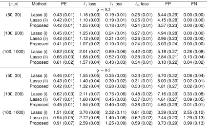
Table 2.1: Means and standard errors (in parentheses) of various performance measures for three methods based on 100 simulations

(n,p) Method PE `1loss `2loss `∞loss FP FN

ρ=0.2

(50, 30) Lasso (i) 0.43 (0.01) 1.16 (0.03) 0.19 (0.01) 0.25 (0.01) 5.44 (0.29) 0.00 (0.00) Lasso (ii) 0.42 (0.01) 1.10 (0.03) 0.19 (0.01) 0.25 (0.01) 4.15 (0.28) 0.00 (0.00) Proposed 0.42 (0.01) 1.05 (0.03) 0.18 (0.01) 0.24 (0.01) 3.57 (0.23) 0.00 (0.00)

ρ=0·5

PE, prediction error; FP, number of false positives; FN, number of false negatives.

distribution (Atchison and Shen, 1980). To reflect the fact that the components of a composition in

metagenomic data often differ by orders of magnitude, we letθ= (θj)withθj=log(0·5p)for j=

1, . . . ,5andθj=0otherwise. To describe different levels of correlations among the components, we

letΣ= (ρ|i−j|)withρ=0·2or0·5. We generated the responses according to model (2.2) withβ∗=

(1,−0·8,0·6,0,0,−1·5,−0·5,1·2,0, . . . ,0)>andσ =0·5, so that three of the six nonzero coefficients

were among the five major components and the rest among the minor components.

We set(n,p) = (50,30),(100,200), and(100,1000), and repeated 100 simulations for each setting.

The tuning parameterλ was selected byGIC as described in§2.3.2. We used six performance

measures for comparisons. The prediction errorky−Zβˆk2₂/nwas computed from an independent

test sample of sizen. The estimation accuracy was assessed by the`qlosseskβˆ−β∗kqwithq=1,2,

and∞. Two variable selection measures were the number of false positives and the number of false

negatives, where positives and negatives refer to nonzero and zero coefficients, respectively. The

means and standard errors of these performance measures for three methods are reported in Table

(29)

As seen from Table 2.1, the lasso (i) estimator has inferior performance in almost all settings, since

the reference component is not regularized and is always included in the selected model. The

lasso (ii) estimator performs better than lasso (i), but always violates the zero-sum constraint in

finite samples. The proposed estimator performs slightly better than lasso (ii) in terms of prediction

and estimation. The variable selection performance of the proposed estimator is comparable to

lasso (ii) with low to moderate dimensionality, but it tends to select fewer false negatives at the

cost of slightly increased false positives in high dimensions. This is reasonable because missing

important variables is more influential than including unimportant variables with shrunk coefficients.

A potential remedy for the violation of the zero-sum constraint in the lasso (ii) estimator would be

to refit the unpenalized linear log-contrast model with the constraint using the selected variables,

which is also useful for reducing the bias caused by the`1penalty. In the Supplementary Material,

we compare the performance of the two-step procedures formed by adding a refitting step to lasso

(ii) or the proposed method, confirming the advantages of our method in the more challenging

settings.

2.5.2. Application to gut microbiome data

Gut microbiome composition is considered an important factor that affects energy extraction from

the diet and contributes to human health and diseases such as obesity. We illustrate the proposed

method by an application to the data set reported in Wu et al. (2011), where a cross-sectional study

of 98 healthy volunteers was carried out at the University of Pennsylvania for investigating

long-term dietary effect on gut microbiome composition. Stool samples were collected on these subjects

and DNA samples were analyzed by 454/Roche pyrosequencing of 16S rRNA gene segments of

the V1–V2 region. The pyrosequences were denoised to yield an average of 9265, with standard

deviation 3864, reads per sample. After taxonomic assignment of the denoised sequences, 3068

operational taxonomic units were combined into 87 genera that appeared in at least one sample.

Since the number of sequencing reads varies greatly across samples, these count data should not

be used directly in a standard regression analysis, and we transformed them into compositional

data after replacing zero counts by the maximum rounding error 0·5 (Aitchison, 2003 §11·5).

De-mographic information including body mass index (BMI) was also collected on these subjects. We

are interested in identifying a subset of important genera whose subcomposition is associated with

(30)

We applied the proposed method to this data set with BMIas the response, and used a refitted

version of tenfold crossvailidation to choose the tuning parameter, where the prediction error for

each sample split was computed with the refitted coefficients obtained after model selection and

without penalization. To obtain stable selection results, we generated 100 bootstrap samples and

applied the same crossvalidation procedure to select the genera. The selection probabilities of

87 genera with bootstrapped crossvalidation are shown in Fig. 2.1(a). Four genera were selected

over 70 times out of the 100 bootstrap replicates. We also followed the approach of stability

se-lection (Meinshausen and B ¨uhlmann, 2010) to assess the stability of the selected genera, where

100 subsamples of size n/2 were taken to compute the selection probabilities. All four genera

had a selection probability greater than 0·85, indicating that the selection results are quite stable.

These four genera along with their selection probabilities and refitted coefficients are presented in

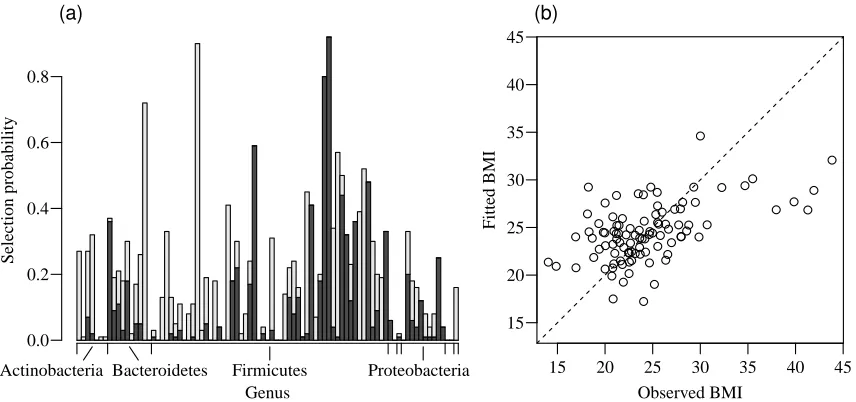
Table 2.2. A plot of the fitted versus observed values ofBMIin Fig. 2.1(b) shows that the model with

four selected genera fits the data reasonably well except for five obese subjects.

(a) (b) Genus 0.0 0.2 0.4 0.6 0.8 Selection probability

Actinobacteria Bacteroidetes Firmicutes Proteobacteria

● ● ●● ● ● ● ● ● ●● ● ● ● ● ● ● ● ● ●● ● ● ● ● ● ● ●● ● ●● ● ● ● ● ● ● ● ● ● ● ● ● ● ● ● ● ● ● ● ● ● ● ● ● ● ● ● ● ● ● ● ● ● ● ● ● ● ● ● ● ● ● ● ● ● ● ● ● ● ● ● ● ● ● ● ● ● ● ● ● ● ● ●● ● ●

15 20 25 30 35 40 45

15 20 25 30 35 40 45 Observed BMI Fitted BMI

Figure 2.1: Analysis of gut microbiome data. (a) Selection probabilities with bootstrapped cross-validation for 87 genera that belong to eight phyla. Selections with a positive sign and a negative sign are shown by dark grey blocks and light grey blocks, respectively; only four major phyla are indicated. (b) Fitted versus observed values ofBMI.

Since our simulations have demonstrated that the lasso (i) estimator is inferior in all respects, we

compare our method only with the lasso (ii) estimator. With selection probabilities above the cutoff

value of 0·7, three genera were selected by lasso (ii) with bootstrapped crossvalidation, which

(31)

Table 2.2: Selection probabilities and refitted coefficients of four selected genera in the gut micro-biome data

Selection probability Refitted

Phylum Genus Boot. CV Stab. Sel. coefficient

Bacteroidetes Alistipes 0.72 0.89 -0.76

Firmicutes Clostridium 0.90 0.96 -1.35

Firmicutes Acidaminococcus 0.80 0.92 -0.61

Firmicutes Allisonella 0.92 0.87 -1.50

Boot. CV, bootstrapped crossvalidation; Stab. Sel., stability selection.

performance of the two methods, we randomly divided the data into a training set of 70 subjects

and a test set of 28 subjects, and used the fitted model chosen by crossvalidation based on the

training set to evaluate the prediction error on the test set. The prediction error averaged over 100

replicates was 30·30 for the proposed method and 30·55 for lasso (ii), with standard errors 0·97 and

1·04, respectively, suggesting that the prediction performance of the proposed method is slightly

better than or similar to that of lasso (ii).

It is interesting to contrast the variable selection results at the phylum level: the proposed method

selected both bacteroidetes and firmicutes as associated withBMI, whereas lasso (ii) selected only

the firmicutes. Thus, our method seems more consistent with the previous finding that the relative

proportion of bacteroidetes to firmicutes is decreased in obese mice and humans by comparison

with lean subjects (Ley et al., 2005, 2006). One biological explanation for the finding as

suggest-ed by metagenomic and biochemical analyses is that the firmicutes-enrichsuggest-ed microbiome holds

a greater metabolic potential than the bacteroidetes-enriched microbiome for more efficient

ener-gy harvest from the diet, which in turn contributes to changes in enerener-gy balance and subsequent

weight gain (Turnbaugh et al., 2006). Furthermore, our selection results at the genus level indicate

that obesity may be associated with changes in gut microbiome composition at a finer taxonomic

level than previously thought.

2.6. Discussion

The linear log-contrast model assumes that the absolute amounts of the covariate components

have no effect on the response. We have adopted this modeling approach in the microbiome data

analysis because the total amount of the microbiome cannot be reliably measured in experiments.

(32)

model in which the total amount also plays a role in affecting the response. To this end, one may

consider the semiparametric varying-coefficient log-contrast model

yi=β0(ai) + p

∑

j=1

βj(ai)logxi j+εi,

p

∑

j=1

βj(ai) =0,

withai being the total amounts. This reduces to model (2.2) when all the coefficientsβ0, . . . ,βpare

constants. A regularized estimation procedure for this model could be developed by combining the

ideas of our approach and the kernel lasso method in Wang and Xia (2012).

Another possible extension of our method for microbiome data analysis would be to take into

ac-count the phylogenetic relationships among the bacterial taxa. Under the biologically plausible

assumption that phylogenetically close taxa tend to have similar effects on the clinical trait, one can

combine the`1penalty in our regularization problem with a Laplacian penalty that encourages

s-moothness among the regression coefficients of closely related taxa on the phylogenetic tree (Chen

et al., 2013). Such an extension is likely to increase the power of identifying important taxa that are

(33)

CHAPTER 3 R

EGRESSION ANALYSIS FOR MICROBIOME COMPOSITIONAL DATA

3.1. Introduction

The human microbiome includes all microorganisms in and on the human body. These microbes

play important roles in human metabolism, nutrient intake and energy generation and thus are

es-sential in human health. The gut microbiome has been shown to be associated with many human

diseases such as obesity, diabetes and inflammatory bowel disease (Manichanh et al., 2012; Qin

et al., 2012; Turnbaugh et al., 2006). Next generation sequencing technologies make it possible

to study the microbial compositions without the need for culturing the bacterial species. There

are, in general, two approaches to quantify the relative abundances of bacteria in a community.

One approach is based on sequencing the 16S ribosomal RNA (rRNA) gene, which is ubiquitous

in all bacterial genomes. The resulting sequencing reads provide information about the bacterial

taxonomic composition. Another approach is based on shotgun metagenomic sequencing, which

sequences all the microbial genomes presented in the sample, rather than just one marker gene.

Both 16S rRNA and shotgun sequencing approaches provide bacterial taxonomic composition

in-formation and have been widely applied to human microbiome studies, including the Human

Micro-biome Project (HMP) (Turnbaugh et al., 2007) and the Metagenomics of the Human Intestinal Tract

(MetaHIT) project (Qin et al., 2010).

Several methods are available for quantifying the microbial relative abundances based on the

se-quencing data, which typically involve aligning the reads to some known database (Segata et al.,

2012). Since the DNA yielding materials are different across different samples, the resulting

num-bers of sequencing reads vary greatly from sample to sample. In order to make the microbial

abundance comparable across samples, the abundances in read counts are usually normalized to

the relative abundances of all bacteria observed. This results in high-dimensional compositional

data with a unit sum. Some of the most widely used metagenomic processing softwares such as

MEGAN (Huson et al., 2007) and MetaPhlAn (Segata et al., 2012) only output the relative

abun-dances of the bacterial taxa at different taxonomic levels.

(34)

identify the bacterial taxa that are associated with a continuous response such as the body mass

index (BMI). Compositional data are strictly positive and multivariate that are constrained to have a

unit sum. Such data are also referred to as mixture data (Aitchison and Bacon-shone, 1984; Cornell,

2011; Snee, 1973). Regression analysis with compositional covariates needs to account for the

intrinsic multivariate nature and the inherent interrelated structure of such data. For compositional

data, it is impossible to alter one proportion without altering at least one of the other proportions.

Linear log-contrast model (Aitchison and Bacon-shone, 1984) has been proposed for compositional

data regression where logarithmic-transformed proportions are treated as covariates in a linear

regression model with the constraint of the sum of the regression coefficients being zero. Lin et al.

(2014) proposed a variable selection procedure for such models in high-dimensional settings and

derived the weak oracle property of the resulting estimates. In analysis of microbiome data, it is also

of biological interest to study the subcompositions of bacteria taxa within higher taxonomic levels,

such as subcompositions of species under a given genus or phylum, or subcompositions of genera

within a phylum. In subcompositional data, the proportions of species have been calculated relative

to total proportions of the species under a given genus; that is, the values in the subcomposition

have been re-closed to add up to 1. Regression analysis of such subcompositional data is also

considered in this chapter.

One of the founding principles of compositional data analysis is that of subcompositional coherence

(Aitchison, 1982): any compositional data analysis should be done in a way that we obtain the same

results in a subcomposition, regardless of whether we analyze only that subcomposition or a larger

composition containing other parts. This is especially relevant in high-dimensional regression

anal-ysis with compositional covariates, where the goal is to select the bacteria whose compositions are

associated with the response. Once such bacteria are identified, it is desirable to recalculate the

subcomposition only within those identified. However, these subcompositions have different values

from those calculated based on a larger set of bacterial taxa. The log-contrast model of Aitchison

and Bacon-shone (1984) and Lin et al. (2014) satisfies this principal by imposing a linear constraint

on the regression coefficients. This chapter extends this model for analysis of microbiome

subcom-positions, where multiple linear constraints are imposed in order to achieve the subcompositional

coherence.

(35)

by James, Paulson, and Rusmevichientong (2015), where the regression coefficients are subject

to a set of linear constraints. A computational algorithm through reformulating the problem as an

unconstrained optimization problem was proposed and non-asymptotic error bounds of the

esti-mates were derived. Different from James, Paulson, and Rusmevichientong (2015), this chapter

presents an efficient computational algorithm based on the coordinate descent method of

multi-pliers and augmented Lagrange of optimization problem. Since the resulting estimates are often

biased due to`1penalty imposed on the coefficients, variance estimation and statistical inference

of the resulting estimates are difficult to derive. In order to make the statistical inference on the

re-gression coefficients and to obtain the confidence intervals, asymptoticly unbiased estimates of the

regression coefficients are first obtained through a de-biased procedure and their joint asymptotic

distribution is derived. The proposed de-biased procedure extends that of Javanmard and

Monta-nari (2014) to take into account the linear constraints on regression coefficients. However, due to

the linear constraints on the regression coefficients, the theoretical developments are different from

Javanmard and Montanari (2014).

Section 3.2 presents linear regression models with linear constraints for compositional covariates.

Section 3.3 presents an efficient coordinate descent method of multipliers to implement the

pe-nalized estimation of the regression coefficients under linear constraints. Section 3.4 provides an

algorithm to obtain de-biased estimates of the coefficients and derives their joint asymptotic

distri-bution. Section 3.5 presents results from an analysis of gut microbiome data set in order to identify

the bacterial genera that are associated withBMI. Methods are evaluated in Section 3.6 through

simulations.

3.2. Regression Models for Compositional Data

3.2.1. Linear log-contrast model

Linear log-contrast model (Aitchison and Bacon-shone, 1984) has been proposed for

composi-tional data regression. Specifically, suppose ann×p matrixXconsists ofn samples of the

com-position of mixture with p components, and supposeY is a response variable depending on X.

The nature of composition makes each row of X lie in a (p−1)-dimensional positive simplex

(36)

Bacon-shone (1984) introduced a linear log-contrast model as follows:

Y=Zpβ\p+ε, (3.1)

whereZp₌_{_log₍_x

i j/xip)} isn×(p−1) log-ratio matrix with the pth component as the reference

component, β\p= (β1, . . . ,βp−1)is the regression coefficient vector, and noiseε is independently

distributed asN(0,σ2). An intercept term is not included in the model, since it can be eliminated by

centering the response and predictor variables.

The selection of reference component is crucial to analysis, especially in high-dimensional settings.

To avoid choosing an arbitrary reference component, Lin et al. (2014) reformulated model (3.1) as

a regression problem with a linear constraint on the coefficients by lettingβp=−∑p_j₌−₁1βj,

Y=Zβ+ε, 1>_pβ =0, (3.2)

where1p= (1, . . . ,1)>∈Rp,Z= (z1, . . . ,zp) = (logxi j)∈Rn×p, andβ = (β1, . . . ,βp)>.

3.2.2. Subcompositional regression model

In analysis of microbiome data, the relative abundances of taxa are often obtained at different

taxonomic ranks, including species, genus, family, class and phylum. It is of interest to study

whether the composition of taxa that belong to a given taxon at a higher rank is associated with

the response, in which case subcompositions of taxa (e.g., all the genera that belong to a given

phylum) are calculated. Supposertaxa at a given rank are considered withmgtaxa at the lower

rank that belong to taxong. LetXgsbe the relative abundance of thesth taxon that belong to thegth

taxon at a higher rank, forg=1,· · ·,r,s=1,· · ·,mgsuch that

mg

∑

s=1

Xgs=1,forg=1,· · ·,r.

Letn×mgmatrixXgrepresentsnsamples of the subcomposition ofmgtaxa. The following model

can be used to link the subcompositions to a responseY,

Y=

r

∑

g=1

Statistical Methods for Compositional and Tree-Structured Count Data in Human Microbiome Studies

University of Pennsylvania

ScholarlyCommons

Publicly Accessible Penn Dissertations

1-1-2016

Statistical Methods for Compositional and

Tree-Structured Count Data in Human Microbiome

Studies

Pixu Shi

Follow this and additional works at:

http://repository.upenn.edu/edissertations

Part of the

Biostatistics Commons

Recommended Citation

Statistical Methods for Compositional and Tree-Structured Count Data in

Human Microbiome Studies

In human microbiome studies, sequencing reads data are often summarized as counts of bacterial taxa at

various taxonomic levels. In this thesis, we develop statistical methods for analyzing such counts data. We first

consider regression analysis with bacterial counts normalized into compositions as covariates. In order to

satisfy the subcompositional coherence of the resulting model, linear models with a set of linear constraints

on the regression coefficients are introduced. A penalized estimation procedure for estimating the regression

coefficients and for selecting variables under the linear constraints is developed. A method is also proposed to

obtain de-biased estimates of the regression coefficients that are asymptotically unbiased and have a joint

asymptotic multivariate normal distribution. This provides valid confidence intervals of the regression

coefficients and can be used to obtain the p-values. Simulation results have shown the validity of the

confidence intervals and smaller variances of the de-biased estimates when the linear constraints are imposed.

The proposed methods are applied to a gut microbiome data set and identify four bacterial genera that are

associated with the body mass index after adjusting for the total fat and caloric intakes.

We then consider the problem of testing difference between two repeated measurements of microbiome from

the same subjects. Multiple microbiome measurements are often obtained from the same subject to assess the

difference in microbial composition across body sites or time points. Existing models for analyzing such data

are limited in modeling the covariance structure of the counts and in handling paired multinomial data. We

propose a new probability distribution for paired multinomial count data, which allows flexible covariance

structure of the counts and can be used to model repeatedly measured multivariate counts. Based on this new

distribution, a test statistic is developed to test the difference in compositions of paired multinomial count

data. The proposed test can be applied to count data observed on taxonomic trees in order to test difference in

microbiome compositions and to identify subtrees with different subcompositions. Simulation results shown

that the proposed test has correct type 1 errors and increased power compared to some commonly used

methods. An analysis of an upper respiratory tract microbiome data set is used to illustrate the proposed

methods.

Dissertation

Doctor of Philosophy (PhD)

Epidemiology & Biostatistics

compositional data, high-dimensional regression, hypothesis testing, microbiome, paired count data,

taxonomic tree

ACKNOWLEDGEMENT

ABSTRACT

TABLE OF CONTENTS

LIST OF TABLES

LIST OF ILLUSTRATIONS

CHAPTER 1

I

1.1. Human microbiome and human health

1.2. Investigating human microbiome through sequencing

1.3. Data structure

1.4. Organization of this thesis

CHAPTER 2

V

2.1. Introduction

2.2. Variable selection in the linear log-contrast model

∑

∑

2.3. Computation

∑

∑

∑

∑

∑

∑

∑

2.4. Theoretical properties

2.5. Numerical studies

2.6. Discussion

∑

∑

CHAPTER 3

R

3.1. Introduction

3.2. Regression Models for Compositional Data

∑

_∑