http://www.sciencepublishinggroup.com/j/ajese doi: 10.11648/j.ajese.20190301.12
ISSN: 2578-7985 (Print); ISSN: 2578-7993 (Online)
Conceptual and Analytic Model for Advanced Evaluation of
Protected Areas’ Global Evolutionary Trends: The
Protected Areas' Trends Assessment and Adaptive
Management on the Basis of Long-Term Conservation
Objectives or PA-TAMCO Analytic Model
Elysée Ntiranyibagira
Integrated Center of Environmental Research, Training and Studies for Development in Africa (ICE-RTSDA), Kigali, Rwanda
Email address:
To cite this article:
Elysée Ntiranyibagira. Conceptual and Analytic Model for Advanced Evaluation of Protected Areas’ Global Evolutionary Trends: The Protected Areas' Trends Assessment and Adaptive Management on the Basis of Long-Term Conservation Objectives or PA-TAMCO Analytic Model. American Journal of Environmental Science and Engineering. Vol. 3, No. 1, 2019, pp. 8-16. doi: 10.11648/j.ajese.20190301.12
Received: December 26, 2018; Accepted: January 15, 2019; Published: February 15, 2019
Abstract:
Protected areas and biodiversity are currently facing important degradation, especially in tropical regions. This evolution questions the management systems and calls for adaptive and sustainable management on the basis of regular assessments of global evolutionary trends and continuous adjustments of conservation objectives and management tools. Adaptive management is yet missing rigorous and integrated indicators for advanced evaluations for many protected areas which have never been assessed despite periodical updating of management goals and plans. The development of reliable, global and low cost methods for adaptive management is therefore a great concern for scientific and conservationist communities given the limitations of commonly used tools and recurrent problems of conservation funding. The PA-TAMCO Analytic Model was designed to promote adaptive actions and management considering spatialized, categorized and aggregated changes from advanced global evaluations. It is an innovative approach and tool for protected areas’ global evolutionary trends with reference to conservation objectives. Theoretically, the Model is based on land cover concepts and land cover analysis recognized as the most practical approach to assess ecosystem units, with reference to vegetation cover, natural processes and theoretical spatial changes. Basically, it relies on four key indicators and tools: (1) Trend Index, (2) Evolutionary Trend, (3) Evolutionary Trend’s Decision Tree Algorithm and (4) Trend Index and Evolutionary Trend’s Classification Grid. Technically, it is based on Remote Sensing data processing; land cover mapping and land cover change analysis using appropriated Remote Sensing and GIS Softwares. The spatial indices and processes responsible for recorded evolutionary trends are determined using landscape ecology tools. In the field of conservation, positive processes are respectively positive and negative when they affect vegetation classes and anthropogenic classes and vice-versa, for negative ones. The input data for the computation of evolution indicators and spatial processes are derived from raw export results of the classifications of Remote Sensing data to GIS software. The sensitivity and resilience of specific ecosystems units to external stresses are measured by three indicators that are “intrinsic stability” (Si), “weighted stability” (Sw) and “relativeexpansion rate” (Re). These indicators are essential for rational management of strategic ecosystems like savannah, water
bodies and wetlands in animal sanctuaries and wildlife parks. The implementation of the Model starts with the knowledge of management category, conservation objectives and desired evolutions. The validation process relies on semi-structured interviews involving technical staff and oldest rangers. The model was successfully applied to the Rusizi National Park (Burundi) from 1984 and 2015.
1. Introduction
Currently, protected areas and biodiversity are facing important and quick degradation worldwide, especially in tropical regions due to continuous human pressures increase and climate change impacts. Climate change is the greatest threats to biodiversity and protected areas networks are natural solutions for adaptation and mitigation [1-2]. It is now proved that 89% of the world's natural ecosystems are already affected by climate change [3]. However, most of protected areas have been established under the assumption of a stable climate [4].
Consequently, the projected climate changes and expected habitats destruction and biodiversity losses call for questioning management hypothesis, goals and plans [3-5] for the protected areas’ adaptive and sustainable management on the basis of periodical assessments of evolutions at global scales. This kind of protected areas’ dynamic and efficient management based on prior knowledge of global evolutionary trends is still missing objective and integrated indicators for rigorous and regular assessments of the evolutionary trends and the effectiveness of the management strategies [6]. It strongly and urgently needs reliable methods, tools and indicators on the management systems, reference made to specific long-term conservation goals [7]. This is as much important as the global evolutionary trends of most of protected areas have never been assessed since their normative classifications, despite regular updating of the management goals and plans, all over the world.
The development of methods for protected areas’ global analysis and assessments is therefore a big concern for the scientific and conservationist communities. Up to now, the most known and used technical tools for the protected areas’ management, monitoring and evaluation are: (1) the “Management Plan” [8-9], (2) the “World Commission on Protected Areas (WCPA)’s Assessment Framework” [6], (3) the “Management Effectiveness Tracking Tool” (METT) developed by IUCN, (4) the “Protected Areas Benefits Assessment Tool” (PA-BAT) developed by WWF and (5) the “African Protected Areas Assessment Tool” (APAAT) [10].
These tools have a certain number of limitations for objective and global assessments due to: (1) the qualitative, subjective and quick character of the evaluations, (2) the restrictive, sectorial or geographical character of the evaluations, (3) the unknown management categories, goals and plans for 85%, 55% and 45% of protected areas, respectively in Africa, in South America and in Europe [11] and (4) the absence of validation, implementation and updating of the rare existing management plans [12].
A lot of protected areas only exist on paper and would be seriously endangered [13]mainly because of: (1) the negative consequences of the still dominant conservation view of "free of people protected areas" [14], (2) the painful evictions and displacements of populations it involves [15, 16, 14], (3) the consequent local poverty and natural resources based conflicts [17-18], (4) the comparative material benefits from
its destruction [19] and (5) the failure or weak performances of participatory management policies and projects [20, 21, 22].
The prioritization of the types of conservation (alpha, beta, gamma) and the recent selective policies for international funding in favor of zones and countries with the greatest tourism and ecological potential [14-23] combined to the great extension of protected areas in number and surface [11] and recurrent problems of national funding that causes the ineffectiveness and inefficiency of the conservation policies in developing countries [24, 14, 23] call for low cost management mechanisms, methods and tools.
The “PA-TAMCO Analytic Model was designed to meet the need of well planned, adaptive and sustainable protected areas management based on global, rigorous, quick and low cost evaluations. It is an analytic tool for regular protected areas assessments and adjustments of management systems, reference made to long-term conservation objectives [7]. The originality and interest of the model is the establishment of global and detailed spatial changes in terms of nature, extent and location, including the physical processes involved and the speed of degradation or development. The model aims to help protected areas Managers to promote well localized corrective or updated actions taking into account the spatialized quantitative and qualitative changes observed between two specific dates. It makes use of the rising facilities and opportunities offered by Remote Sensing platforms and open access and free of charge global land products, given the fact that traditional field methods for biodiversity monitoring and analysis require heavy, expert and expensive inventories [25] which do not allow easy data and management plans updating because of the inadequacy and low quality of the data [26].
2. Methodological Approach
2.1. Theoretical and Operational Framework of PA-TAMCO Analytic Model
dynamics and degradation processes [40-41].
The landscape transformations determine the general evolutions and levels of fragmentation, connectivity and spatial heterogeneity while spatial characteristics of patches influence ecological processes such as migrations, predation, extinction and colonization [42]. The fragmentation process reduces the surface and quality of habitats and creates or reinforces gaps in continuity [43-44]. It limits the chances of species survival in isolated fragments. The habitat diversity is therefore one of the best ecological values of ecosystems [45].
The PA-TAMCO Model is based on that assumption and on the 2main characteristics of protected areas: (1) the existence of physical boundaries and (2) the existence of a mechanism for recognition and management [46]. The model relies theoretically and operationally on the following land cover concepts: (1) Land cover [47-48], (2) Land cover Transition matrix [49], (3) Land cover stability [50], (4) Land cover modification [38, 39, 51, 48] and (5) Land cover conversion [39, 51, 48].
Some of the basic concepts have been nuanced or reconceptualized to describe better the ecological and spatial dynamics at work in protected areas’ landscapes. In the model, the "Land cover modification" has been split into: (1) "positive modification" and (2) "negative modification". The positive modification is defined as "the shift or the surface transfer from a less dense vegetation class to a dense vegetation class or from a less developed vegetation formation to a more developed vegetation formation", as opposed to negative modification, with reference to the natural and spontaneous succession of vegetation [52]. For the same purpose, the "Land cover conversion" has been divided into: (1) "non-vegetal conversion", (2) "positive conversion" and (3) "negative conversion". The non-vegetal conversion is considered as "the shift or surface transfer from a non-vegetal class to another one", the positive conversion "the shift or surface transfer from a non-vegetal class to a class of vegetation" and the negative conversion, the reverse. In other words, the positive and negative conversions are respectively directed towards physical appearances and disappearances of the vegetation cover, whatever their nature and stage of development.
In theory, protected areas and natural ecosystems can be affected by six kinds of spatial transformations which are: (1) stability (no spatial change), (2) non-vegetal conversion (conversion between non vegetal land cover classes), (3) positive conversion (vegetation appearance or quantitative gain
of vegetation) (4) negative conversion (vegetation
disappearance or quantitative loss of vegetation), (5) positive modification (qualitative gain of vegetation) and (6) negative modification (qualitative loss of vegetation). In terms of global evolutions in vegetation cover, “non-vegetal conversions” are neutral (neutral conversions), “positive conversions and modifications” a "progression of vegetation" and “negative conversions and modifications” a "regression of vegetation". Habitats and vegetation cover being the key components of biodiversity stricto sensu [28] and their developments or stabilities the main conservation goals, the “regression of vegetation " and "neutral conversions" are negative evolutions
for the conservation. At contrary, the "progression of vegetation" and "land cover stabilities" are positive evolutions for the conservation. The second option explains the dominating position of protected areas under the management categories I, II, III and IV [11] known as natural areas or largely natural areas exposed to natural processes [53-23].
The PA-TAMCO Analytic Model is technically based on the processing and analysis of Remote Sensing images and land cover mapping for the identification of land cover classes and periodical land cover changes [54, 55, 56, 57]. The Remote Sensing data can be of low, medium or high spatial resolutions; depending on their availability and cost, the size of a specific protected area and the degree of accuracy expected for the assessment. Preferably, the data are acquired at the beginning of the dry season to avoid noisy images and allow maximal differentiation of land cover classes, especially between herbaceous and woody [26-57]. The importance and interest of Remote Sensing data and GIS techniques associated with eco-landscape structure tools for the study and monitoring of natural ecosystems are widely recognized [58, 54, 59] compared to in situ or direct methods which are costly and technically demanding [23].
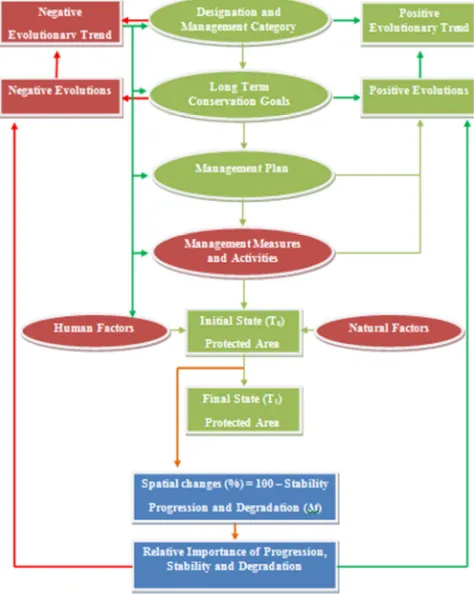
Figure 1. Protected Areas’ Sustainable Management Modeling.
continuously acting. The type and the relative importance of aggregated land cover changes between the initial state and the final one make it possible to determine the evolutionary trends which are either positive when they carry out the desired evolutions or negative when they lead to contrary evolutions. As a result of assessment, management gaps and negative evolutions observed command new or updated management category, conservation objectives, management plan and management measures and activities and so on, as indicated in Figure 1.
2.2. PA-TAMCO Model’s Core Indicators: Trend Index and Evolutionary Trend
Basically, PA-TAMCO Analytic Model relies on two core indicators for the description of protected areas’ historical evolutions. These are: (1) the Trend Index (Ti) and (2) the Evolutionary Trend (Et). The protected area’s “Trend Index”
is a synthetic indicator which quantifies and qualifies the global Evolutionary Trend of a protected area over a period of time in order to assess the effectiveness of conservation strategies and to ensure adaptive management to face increasing climatic and human stresses. The basic principle of the methodological approach used for the determination of the Trend Index is the adjustment of the quantitative and qualitative spatial changes affecting land cover classes to long-term conservation objectives [7]. The “Evolutionary Trend” is an expressive interpretation of the Trend Index
values and classes. It is a combinatorial reading of the labels of spatial change rates and spatial change balances (Table 1) expressed by a "quantitative and qualitative synthetic formulation" which clearly reflects the “intensity of spatial changes” and the “level of balanced protected area’s evolutions”, in terms of progressions (developments), stabilities (no spatial change) and regressions (degradations).
2.3. Trend Indices and Evolutionary Trends Computation
The computation process consists of three successive stages. First, it starts with the processing and analysis of multi-temporal Remote Sensing data using appropriate Softwares. The results of classifications of images are then vectorized and exported to GIS Softwares for further cartographic analysis. Secondly, the process determines the spatial transformations and the surface transfers between land cover classes from date T0 to date T1
thanks to cartographic and transition matrix analysis. Let’s consider a theoretical example of a protected area made of 6 pure or combined land cover classes A1, A2, A3, A4, A5 and A6
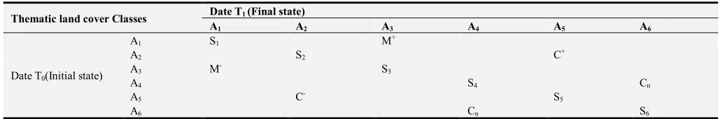
just for illustration. The transition matrix presented below provides possible types of spatial transformations existing between land cover classes (Table 1). According to the conservation goals, the nature of land cover classes and their respective meanings for the conservation, the operator decides on the status to be allocated to each spatial transformation affecting land cover classes, couple by couple. In other words, each cell is allocated one of the six theoretical spatial changes.
Table 1. Theoretical Land Cover Transition Matrix from date T0 to date T1 (%).
Thematic land cover Classes Date T1 (Final state)
A1 A2 A3 A4 A5 A6
Date T0(Initial state)
A1 S1 M+
A2 S2 C+
A3 M- S3
A4 S4 Cn
A5 C- S5
A6 Cn S6
For any couple of land cover classes Ai and Aj, if the shift
from Ai to Aj is a positive modification (M +
), then the shift from Aj to Ai is a negative modification (M-) and vice-versa. If the
shift from Ai to Aj is a positive conversion (C+), then the shift
from Aj to Ai is a negative conversion (C-) and vice-versa. If the
shift from Ai to Aj is a neutral conversion (Cn), then the shift
from Aj to Ai is a neutral conversion too (Cn). The proportion of
pixels of the class Ai which do not change of land cover type is
the stability of the class (Si). After considering all the
combinations of coupled land cover classes and determining the different proportions of M+, M-, C+, C- and Cn(%), then the
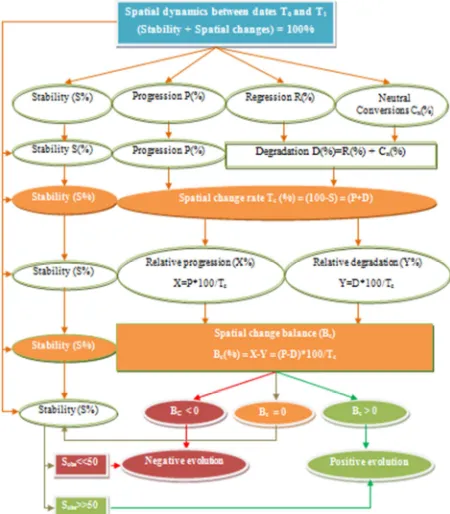
operator moves to the third stage of the computation process which is an aggregation of these quantities at the global level of a protected area. The aggregation process provides the values of the synthetic statistics or global parameters of landscape dynamics S, P, R and Cn from which advanced parameters D, X,
Y, Tc and Bc are computed (Figure 2). It also leads to the
mapping of global land cover changes in terms of overall stability, neutral conversions, regression of vegetation and progression of vegetation. The synthetic statistics are derived from cartographic analysis and related land cover Transition
matrices as described above in Table 1. Their values result from
the equations: (1) = ∑ + ∑ , (2) = ∑ M +
∑ C , (3) = ∑ Sand (4) = ∑ Cn where M-, M+, C-, C+, S and Cn are the theoretical spatial evolutions defined above.
Finally, the computation of the Trend Index is based on the comparison of the overall proportions of “regressions of vegetation” (R), “progressions of vegetation” (P), “neutral conversions” (Cn) and “protected area’s stability” (S) which
constitute the input data in the computational model (Figure 2). The Trend Index incorporates 3 variables: "spatial change rate "(Tc), "change dominating direction" and "change balance value
(Bc)". The variable Tc represents the proportion of spatial
difference between the two quantities. When " # 0, the Evolutionary Trend (Et) is positive. When " $ 0 , the
Evolutionary Trend is negative. If" = 0, the Evolutionary Trend is determined by the relative importance of spatial change rate Tc and the global stability S. Here, the threshold value
considered for the stability (Ss) is equal to 50%. This is the
solution of the equation (6) % = & ⟺ % = 100 − &. Assuming that in the field of conservation "stability is less than a progression and better than a degradation", we consider that for equal relative progression and degradation corresponding to the equation (7)( − Y = 0 ⟺ Bc = 0, the better the stability is, the better the evolution for the conservation is and vice versa. If the measured stability Sobs ≥ Ss, the Evolutionary Trend (Et) is
positive. Otherwise, it is negative (Figure 2).
Figure 2. Trend Indices and Evolutionary Trends’ Decision Tree Algorithm.
2.4. Trend Indices and Evolutionary Trends Classification Grid
The values of variables Tc and Bc resulting from the
calculations are placed in the appropriate cells of the Trend Index Classification Grid where columns and rows represent respectively the spatial change rate and the spatial change balance. In the Classification Grid, the spatial change rates are divided into 4 classes of 25% intervals, which mean from 0% to 100%"a low evolution" coded (1), "a moderate evolution" coded (2), "a strong evolution" coded (3) and " a very strong evolution" coded (4). The spatial change balances are divided into 8 classes of 25% intervals with 4 classes of negative values at the top of the table and 4 classes of positive values at the bottom of the table (Table 2).
The negative balance classes mean from -100% to 0%, "a very strong negative trend" coded (a), "a strong negative trend" coded (b), "a moderate negative trend" coded (c) and “a low negative trend” coded (d). The positive balance classes express from 0% to 100% "a low positive trend" coded (D), “a moderate positive trend" coded (C), "a strong positive trend" coded (B) and "a very strong positive trend" coded (A). The classes of negative balances (a to d) and positive balances (D to A) are symmetrical with respect to the value axis " = 0 (6). The Trends Indices are alphanumeric combinations ranging from (1d) to (4a) for extreme negative trends and (1D) to (4A) for positive trends (Table 2). For example, a Trend Index of Ti [(77, -64), 4b] corresponds to “a
very strong evolution (4)" with “a strong negative trend (b)" which is characterized by spatial changes affecting 77% of a protected area’s surface, consisting of 82% degradation and 18% progression, resulting in an overall negative evolution of 64%. When the value of " = Yis known, P and D are
determined by solving the system of equations: (1) + , =
100 and (2) − , = -of which solutions are: =. / 0
and , = . 1
0 .
Table 2. Trend indices and Evolutionary trends Classification Grid.
Variables Spatial change rates (Tc %)
[0-25] [25-50] [50-75] [75-100]
Change balance (Bc%)
Degradation
[-100,-75] 1a 2a 3a 4a
[-75,-50] 1b 2b 3b 4b
[-50,-25] 1c 2c 3c 4c
[-25, 0] 1d 2d 3d 4d
Progression
[0-25] 1D 2D 3D 4D
[25-50] 1C 2C 3C 4C
[50-75] 1B 2B 3B 4B
[75-100] 1A 2A 3A 4A
Period Methodology and steps for indices values computation Trend indices
∆t {Tc= (100-S) = x ϵ] α-β] class i; Bc = (X-Y) = yϵ [γ-δ] (>, <) 0 class j} It = [(x, y); ij]
2.5. Spatial Transformation Processes and Fragmentation Measurement
The observed land cover changes, landscape dynamics and
[64].
On a physically and theoretical basis, patch aggregation, creation and enlargement are “positive processes”; patch dissection, fragmentation, attrition, perforation and shrinkage “negative processes” and patch deformation and shift “neutral processes”[65, 66, 61, 63]. However, in the field of conservation and protected areas management, these spatial processes have to be interpreted differently depending on whether they affect vegetation classes or anthropogenic classes. So-called positive processes are “positive” when they affect vegetation classes and “negative” when they affect anthropogenic classes and vice versa, for so-called negative processes.
In case of patch fragmentation and patch dissection processes, the computation of the patch dominance of the land cover classes [67] completes the knowledge of the spatial processes by establishing the levels of patch fragmentation or consolidation, especially for the vegetation classes. In the area of conservation and protected areas management, the interpretation of the variation of patch dominance depends on the type of land cover. When the patch dominance of a land cover class is increasing between 2 dates, the evolution is “positive” if the consolidation goes to vegetation classes. Conversely, it is “negative” if it affects anthropogenic classes and vice-versa, for patch dominance decrease.
The input and analytic data for the computation of the spatial structure indices and the determination of the spatial transformation processes are the patch number (N), area (A) and perimeter (P) derived from Open Attribute Table resulting from the raw export results of the classifications of Remote Sensing images to GIS software. The input and analytic data for the computation of the patch dominance and the patch dominance variations are the biggest patch area (At) and the area of the related class (Am) resulting from the
same Open Attribute Table.
2.6. Ecosystems Resilience’s Indicators: Intrinsic Stability, Weighted Stability and Spatial Expansion
The resilience of specific ecosystems and habitats are measured by three core indicators: (1) the “Intrinsic stability” (Si), (2) the “Weighted stability” (Sw) and (3) the “Relative
Annual Expansion Rate” (Re). The stability of an ecosystem
or a land cover class can be defined at three levels: (1) the “absolute stability” or the “stability” stricto sensu (Sa) which
is the proportion of stable pixels of the class from date T0 to
date T1, (2) the “intrinsic stability” (Si) which is the ratio
between the absolute stability (Sa) and the coverage rate of
the class in the protected area at date T0 and (3) the "weighted stability" (Sw) which represents the ratio between the
“Equivalent coverage rate” of the class at date T1 and the
“coverage rate of the class" at date T0. The “Equivalent coverage rate” of a class is defined as the proportion of the
absolute stability (Sa)in the global stability of a protected
area (S). The weighted stability (Sw) measures the relative
stability of a given ecosystem or habitat compared to its
weighted importance or coverage in the protected area’s total
surface and overall stability. Important levels of weighted stability (Sw> 100%) indicate a proportionally high stability
of an ecosystem compared to the global spatial transformations affecting the protected area as a whole and vice-versa, for lower levels (Sw< 100%).
The differential or comparative sensitivity of a specific ecosystem, habitat or land cover class to climatic conditions and socio-economic related stresses is measured by the “relative annual expansion rate” (Re) (%/year/ha) which is
defined as the “annual average speed of development or degradation” between date T0 and date T1, with reference to
its initial area (A) at date T0. It is determined by the
following relation: 2 =34
5 [22] where A0 is the area (ha) at
date T0 and Ta the “mean annual expansion rate” a defined
by the formula: a = 100 ∗ 9. :
9 %3. 3 & [68] where S0 and S1
are the areas of the land cover class respectively at dates T0
and T1. Additionally to the determination and the knowledge
of Trend Indices and global Evolutionary Trends over a period of time, these environmental indicators are for example essential for the measurement of the degree of development, stability and degradation of strategic ecosystems like rainforests, savannah, water bodies and wetlands and aesthetic landscapes in most of animal sanctuaries or wildlife parks in Africa that mobilize tourism industries and conservation budgets [14]. The development and rational management of such ecosystems are life and sustainability insurance both for tourism and socio-economic development.
2.7. PA-TAMCO Analytic Model’s Validation Process
In the framework of PA-TAMCO Analytic Model, the validation process of the Evolutionary Trends is done through two complementary levels: (1) Individual interviews involving the technical staffs who have managed or are still managing interested protected areas during the periods covered by the assessment and (2) Semi-structured focus group interviews involving the protected areas’ oldest rangers in place since the longest time possible. The interviews are based on the Trend Index and Evolutionary Trends Classification Grid (Table 2) for easy understanding and quick interpretation of the protected areas’ evolutions by managers and rangers. The validation process is intended to precise the kind and the importance of the global evolutions in terms of spatial changes “amplitude” and “dominating direction”.
2.8. PA-TAMCO Analytic Model’s Probationary Test
respectively Ti [(38%, 6%), 2D], Ti [(77%, -82%), 4a], Ti
[(65%, 22%), 3D], Ti [(58%, -36%), 3c] and Ti [(77%,
-64%), 4b]. The periodical Evolutionary Trends of the Rusizi National Park corresponding to these Trend Indices and periods were respectively: a "moderate evolution (2) with a low positive trend (D)", a "very strong evolution (4) with a very strong negative trend (a)”, a "strong evolution (3) with a low positive trend (D)”, a “strong evolution (3) with a moderate negative trend (c)” and a “very strong evolution (4) with a strong negative trend (b)”. The final findings were all validated and confirmed through semi-structured individuals and focus group interviews involving the successive Park’s Managers and the Park’s oldest Rangers who have been continuously in place since the creation of the Park in 1980 under the status of Natural Forest Reserve.
3. Conclusion
The protected areas’ adaptive and sustainable management requires regular evaluations and continuous adjustments of management objectives, methods and tools. The PA-TAMCO Model is an integrated, innovative and low cost approach which was designed for advanced evaluations of global evolutionary trends to achieve that goal. Compared to current assessment methods and tools, the originality and interest of the Model is the establishment of the precise nature, categories and extent of quantitative and qualitative spatial changes for well inspired, rational and localized corrective actions. The Model is then a good response to the lack of rigorous methods and indicators for global evolutionary trends ‘assessments and to the increasing need for efficient and low cost methods to face current technical constraints and recurrent problems related to international and national funding. The facilities offered by Remote Sensing platforms and open access and free of charge data constitute a remarkable opportunity for the successful implementation of the Model to all kind of protected areas. Indeed, the importance and interest of Remote Sensing data and GIS techniques for the study and monitoring of natural ecosystems as essential strategies and guarantees for biodiversity management are widely recognized, compared to heavy, expert and costly inventories required by in situ or direct methods. In the field of conservation and protected areas management, the Model shows that spatial processes should be interpreted differently depending on whether they affect vegetation classes or anthropogenic classes. It also stated that the measurement of the sensitivity or resilience of specific ecosystems units to external stresses are essential for the management of strategic ecosystems, especially in animal sanctuaries and wildlife parks to support tourism industry and activities. Given its interest and precision, it is crucial to use the Model for the assessment of protected areas’ global evolutionary trends before updating conservation objectives and management plans. For this purpose, training sessions are needed for capacity building at national, regional and international levels.
References
[1] IPCC (2007). Climate Change 2007: Impacts, Adaptation and Vulnerability. Contribution of Working Group II to the Fourth Assessment Report of the Intergovernmental Panel on Climate Change, M. L. Parry, O. F. Canziani, J. P. Palutikof, P. J. van der Linden and C. E. Hanson, Eds., Cambridge University Press, Cambridge, UK, 976 pp.
[2] Dudley N., Stolton S., Belokurov A. and al. (2010). Natural solutions: Protected areas helping people cope with climate change. Gland (Switzerland), Washington DC and New York (USA): IUCN-WCPA, TNC, UNDP, WCS. The World Bank, WWF, 130p.
[3] McCarty J. P. (2001). Ecological consequences of recent climate change. Conservation Biology, 15: 320–331.
[4] Hannah L. and Salm R. (2005). Protected areas management in a changing climate. In: Lovejoy T. E. and Hannah L. (eds.) Climate change and biodiversity. New Haven and London: Yale University press, 440p.
[5] Hopkins J. J., Allison H. M., Walmsley C. A. and al. (2007). Conserving Biodiversity in a Changing Climate: guidance on building capacity to adapt, Department of Environment, Food and Rural Affairs, London, 32p.
[6] Hocking M. and Phillips A. (1999). How well are we doing? Some thoughts on the effectiveness of protected areas. Parks, 9 (2): 5-14.
[7] Hockings M., Stolton S., Leverington F. and al. (2006). Evaluating Effectiveness: A Framework for Assessing Management Effectiveness of ProtectedAreas, SecondEdition. N°14. UICN, Gland, Suisse. xiv + 105p.
[8] Mackinnon J. K., Mackinnon G. C et Thorsell J. (1990). Aménagement et gestion des aires protégées tropicales, UICN, Suisse, 307p.
[9] Chiffaut A. (2006). Guide méthodologique des plans de gestion deréserves naturelles. MEED/ATEN, Cahier technique N°79: 72p.
[10] Hartley A., Nelson A., Mayaux P. and al. (2007). The Assessment of African Protected Areas. EUR 22780. A characterization of biodiversity value, ecosystems and threats, to inform the effective allocation of conservation funding. EN, Luxembourg: Office for Official Publications of the European Communities, 80p.
[11] Deguignet M., Jufe-Bignoli D., Harrison J. et al. (2014). Liste des Nations Unies des Aires Protégées 2014. UNEP-WCMC: Cambridge, UK, 44p.
[12] UICN (2012). Cadre et outils d’évaluation de l’efficacité de la gestion des aires protégées en Afrique de l’ouest et du centre. Programme Afrique Centre et Ouest, 21p.
[13] Binot A. (2010). La Conservation de la Nature en Afrique Centrale. Entre Théories et Pratiques. Des Espaces Protégés à Géométrie Variable. Thèse de Doctorat, Université Paris 1 Panthéon-Sorbonne, 444p.
[15] Neumann R. P. (1998). Imposing Wilderness: struggles over livelihood and nature preservation in Africa, Los Angeles and Berkeley: University of California Press, 268 pp.
[16] Rossi G. (2000). Ingérence écologique. Environnement et développement rural du Nord au Sud. CNRS Editions Coll. Espaces et Milieux, Paris, 248p.
[17] Besong J. B. and Wencélius F. L. (1992). Realistic strategies for conservation in the tropical moist forests of Africa: regional review. In Cleaver, C., Munasinghe, M., Dyson, M, Egli, N, Peuker, A. and Wencélius, F. (Eds.). Conservation of West and Central African Rainforests. The World Bank, Washington, D. C. pp. 21-31.
[18] Sournia G. (1996). Les aires protégées d'Afrique francophone (Afrique centrale et occidentale). Hier, aujourd'hui, demain. Espaces à protéger ou espaces à partager ? Thèse de doctorat, Bordeaux, Université de Bordeaux III, 302p.
[19] Ferraro P. J. and Kiss A. (2002). Getting what you paid for: direct payment an alternative investment for conserving biodiversity, Science n 268, November 29, 2002.
[20] Binot A. et Joiris D. V. (2007). Règles d’accès et gestion des ressources pour les acteurs des périphéries d’aires protégées. VertigO - la revue électronique en sciences de l'environnement [En ligne], Hors-série 4|novembre 2007, mis en ligne le 11 novembre 2007, URL: http://vertigo.revues.org/759; DOI: 10.4000/vertigo.759
[21] Borrini-Feyerabend G., Dudley N., Jaeger T. and al. (2013). Governance of Protected Areas: From understanding to action. Best Practice Protected Area Guidelines, Series 20, Gland, Switzerland: IUCN, xvi, 124p
[22] Ntiranyibagira E. (2017). Dynamiques d’occupation du sol, tendances évolutives globales et facteurs d’évolution des aires protégées. Etude diachronique du Parc national périurbain de la Rusizi (Burundi) de 1984 à 2015. Thèse de Doctorat Unique en Sciences de l’Environnement, Université Cheikh Anta Diop de Dakar (Sénégal), 340p.
[23] Aubertin C. et Rodary E. (2008). Aires protégées, espaces durables ? IRD, 276p
[24] James A. N (1999). Institutional constraints on protected area funding. Parks, 9(2): 15-26.
[25] Howard P., Davenport T., Kigenyi F. and al. (2000). Protected area planning in the tropics: Uganda's national system of forest reserves. Conservation Biology, 14: 858-875.
[26] Sambou B. (2004). Evaluation de l’état, de la dynamique et des tendances évolutives de la flore et de la végétation ligneuses dans les domaines soudanien et sub-guinéen au Sénégal. Thèse de Doctorat d’Etat en Sciences Naturelles. Université Cheikh Anta Diop de Dakar (Sénégal), 209p.
[27] Noss R. F. (1996). Ecosystems as conservation targets. Trends in Ecology & Evolution, 11:351.
[28] Cowling R. M., Knight A. T., Faith D. P. and al. (2004). Nature conservation requires more than a passion for species. Conservation Biology, 18:1674-1676.
[29] Chape S., Harrison J., Spalding M. and Lysenko I. (2005). Measuring the extent and effectiveness of protected areas as an indicator for meeting global biodiversity targets.
Philosophical Transactions of the Royal Society B 360: 443-455.
[30] Fahrig L. (2003). Effects of habitat fragmentation on biodiversity. Annual Review of Ecology, Evolution and Systematics, 34: 487-515.
[31] Henle K., Lindenmayer D. B., Margules C. R. and al. (2004). Species survival in fragmented landscapes: Where are we now? Biodiversity and Conservation, 13: 1-8.
[32] Clerici N., Bodini A., Eva H. and al. (2007). Increased Isolation of Two Biosphere Reserves and Surrounding Protected Areas (WAP: W-Arly-Pendjari, Ecological Complex, West Africa). Journal of Nature Conservation, 15: 26-40.
[33] Jeremy B., Youssoufou S., Yahaya S. and al. (2007). Identification of ecological indicators for monitoring ecosystem health in the trans-boundary W Regional Park: A pilot study. Biological Conservation, 238: 73-88.
[34] Tilman D., May R. M., Lehman C. L. and al. (1994). Habitat destruction and the extinction debt. Nature, 371:65-66.
[35] Terborgh, J. and van Schaik C. P. (1997). Minimizing species loss: the imperative of protection. In Kramer R., van Schaik C. and Johnson J. éds. Last stand: protected areas and the defense of tropical biodiversity, University of Oxford Press, Oxford, United Kingdom, 15-35.
[36] Rodríguez J. P., Balch J. K. and Rodríguez-Clark K. M. (2007). Assessing extinction risk in the absence of species-level data: quantitative criteria for terrestrial ecosystems. Biodiversity and Conservation, 16: 183-209.
[37] Eva H. D., Brink A. B. and Simonetti D. (2006). Monitoring land cover dynamics in Sub-Saharan Africa. A pilot study using Earth observing satellite data from 1975 and 2000. JRC Scientific and Technical Reports, 40p.
[38] Stott A. and Haines-Young R. (1996). Linking land cover, intensity of use and botanical diversity in an accounting framework in the UK.
[39] Alun J. and Clark J. (1997). Driving forces behind European land use change: an overview. Claude Resource Paper n° 1.
[40] Lambin E. F., Turner B. L., Geist H. and al. (2001). The Causes of Land-Use and Land-Cover Change: Moving beyond the Myths. Global Environmental Change, 11: 261-269.
[41] Rodríguez J. P., Rodríguez-Clark K. M., Baillie J. E. M. et al. (2011). Elaboration des Critères de l’UICN pour la Liste Rouge des Ecosystèmes Menacés. Conservation Biology, Volume25, 11p.
[42] Farina A. (2000). Landscape ecology in action. Kluwer Academic Publishers, Dordrecht. The Netherlands, 267p.
[43] Davidson C. (1998). Issues in measuring landscape fragmentation. Wildlife Society Bulletin, 26: 32-37.
[44] Burel F. et Baudry J. (2003). Ecologie du paysage. Concepts, méthodes et applications. Paris: France, Tec & Doc. 359 pp.
[45] Lockwood M., Worboys L. G. and Kothari A. (2006). Managing Protected Areas: A Global Guide. London Earthscan, IUCN, xxx, 802 pp.
[47] Di Gregorio A. and Jansen L. J. M. (1997). A new concept for a Land Cover Classification System. Earth observation and evolution classification. Compte rendu de la conférence des 13-16 octobre 1997. Alexandrie, Égypte, 10 p.
[48] CEC (2001). Manuel des concepts relatifs aux systèmes d’information sur l’occupation et l’utilisation des sols. Luxembourg, Office des Publications officielles des Communautés européennes. Thème 5: Agriculture et Pêche, Edition 2000, 96p.
[49] Robin M. (2002). Télédétection, des satellites au SIG. Une analyse complète du processus de création d’un type essentiel d’information géographique. Nathan Université. ISBN: 2 -0919-1224-7, 318p.
[50] Barima S. S. Y., Barbier N., Bamba I. et al. (2009). Dynamique paysagère en milieu de transition forêt-savane ivoirienne. Bois et forêt des tropiques, 63 (299) : 15-25.
[51] Baulies X. I. and Szejwach G. (ed.) (1997). Survey of needs, gaps and priorities on data for land use and land cover change research. LUCC Data requirements workshop, Barcelone, November, 11-14, 1997, LUCC report series 3.
[52] ITTO (2002). “Reintegrate secondary forests into the landscape”. ITTO Tropical Forest Update 10/4/2002.
[53] Locke H. and Dearden P. (2005). Rethinking protected area categories and the new paradigm. Environmental Conservation, 32 (1): 1-10.
[54] Girard, M. C et Girard C. (1999). Traitement des données de télédétection. Paris, Ed. Dunod, ISBN: 2 -1000-4185-1,529p.
[55] Mas J. F. (2000). Une revue des méthodes et des techniques de télédétection du changement. Canadian Journal of Remote Sensing, 26 (4): 349-362.
[56] Galicia L. and Garcia-Romero A. (2007). Land use and land cover change in Highland temperate forests in the Izta-Popo national park, central Mexico. Mountain Research and Development, 27 (1): 48-57.
[57] Tabopda W. G. and Fotsing J. M. (2010). Quantification de l’évolution du couvert végétal dans la réserve forestière de Laf-Madjam au nord du Cameroun par télédétection satellitale. Sécheresse, 21 (3): 169-178.
[58] Ulbricht K. A. and Heckenford W. D. (1998). Satellite images for recognition of landscape and land uses changes.
Journal of Photogrammetry and Remote Sensing, vol.53: 235-243
[59] Mayaux P., Eva H. D., Palumbo I. et al. (2007). Apport des techniques spatiales pour la gestion des aires protégées en Afrique de l’Ouest. In : Fournier A., Sinsin B., Mensah G. A. (éds). Quelles aires protégées pour l’Afrique de l’Ouest ? Conservation de la biodiversité et développement. Paris, IRD, coll. Colloques et séminaires, p.321-328.
[60] Hargis C. D., Bissonette J. A. and David J. L. (1997). Understanding measures of landscape pattern. In: Wildlife and landscape ecology (eds. Bissonette J. A.), pp. 231-261. Springer, Berlin Heidelberg, New York.
[61] Jaeger J. A. G. (2000). Landscape division, splitting index, and effective mesh size: new measures of landscape fragmentation. Landscape Ecology, 15:115–130.
[62] Fortin M. J. (2002). Spatial analysis in ecology: statistical and landscape scale issues. Ecoscience, 9: iii-v.
[63] Bogaert J., Ceulemans R. and Salvador-Van Eysenrode D. (2004). Decision tree algorithm for detection of spatial processes in landscape transformation. Environment Management, 33(1): 62-73.
[64] Hansson L. and Angelstam P. (1991). Landscape ecology as a theoretical basis for nature conservation. Landscape Ecology, 5 (4): 191-201.
[65] Forman R. T. T. (1995a). Land mosaics—the ecology of landscapes and regions. Cambridge University Press, Cambridge, 632p.
[66] Collinge S. K. and Forman R. T. T. (1998). A conceptual model of land conversion processes: predictions and evidence from a micro landscape experiment with grassland insects. Oikos, 82: 66–84.
[67] McGarigal K. and Marks B. J. (1995). Fragstats: Spatial Pattern Analysis Program for Quantifying Structure. Department of Agriculture, Pacific Northwest Research Station General Technical Report PNW-GTR-351. Oregon, USA.