Relationship Between GDP And GDS In The UAE: ARDL Bound Testing Approach

(1)

DOI: 10.14738/abr.67.4895.

Hussain, M. A., & Saaed, A. A. J. (2018). Relationship Between GDP And GDS In The UAE: ARDL Bound Testing Approach.

Archives of Business Research, 6(7), 192-203.

Relationship Between GDP And GDS In The UAE:

ARDL Bound Testing Approach

Majeed Ali Hussain

Professor of Econometrics,

College of Business Administration American University in the Emirates United Arab Emirates. Dubai International Academic City

Afaf Abdull J. Saaed

Associate Professor of Applied Economics,

College of Business Administration American University in the Emirates. Dubai International Academic City

ABSTRACT

This study explores the relationship between Gross Domestic Product (GDP) and Gross Domestic Saving (GDS) in United Arab Emirates (AUE covering the period 1980 – 2013, using the autoregressive distribution lag (ARDL) cointegration framework. Granger Causality test were employed in the empirical analysis. Using Augmented Dickey-Fuller (ADF) and Phillip-Perron (PP) stationarity test, the variable proved to be integrated of the order one 1(1) at first difference. The results based on the bounds testing procedure confirm that a long-run relationship between GDP and GDS exist. The results indicate that domestic savings is significantly positively related to growth in UAE These results are consistent with the findings of Mphuka (2010), Abu (2010), Nurudeen (2010) and Mohan (2006). The econometric evidence that LGDS causes LGDP and there is evidence that saving is the driver of economic growth in UAE. Considering the findings mentioned above, we make the following recommendations; Measures to increase growth and economic diversification in UAE should aim to promotes domestic savings and increases domestic savings overall. Fiscal and Monetary policies that allow for increased savings and that enhances domestic savings is vital. The study recommends the need for development of financial instruments to encourage domestic savings.

Keywords: Savings; Economic Growth; Bounds; Cointegration; UAE.

INTRODUCTION

(2)

suggest appropriate economic growth policies. To address this issue, we draw on recent Gross Domestic savings- economic growth modelling literature and examine the Gross Domestic savings and economic growth relationship in UAE using data from 1980- 2013. This study utilizes an ARDL bounds testing approach to cointegration to determine both the long run and short run impacts of Gross Domestic savings on economic growth.

In the empirical literature, the issue of the relationship between Gross Domestic savings (GDS)

and economic growth (GDP has attracted a lot of academic interest from different parts of the world (Abu Al-Foul, 2010; [9]; Masih & Peters, 2010 [10]; Tang & Tan, 2014) [11]and central to

this relationship is the issue of causation. While some studies have reported causality running

from saving to growth (Alguacil et al., 2004 [12]; Anoruo & Ahmad, 2001[13]; Olajide, 2010 [14]; At the same time, we have studies that report bidirectional relationship (AbuAl-Foul, 2010 [9]; Zeren & Ekrem, 2013) [15]. Meanwhile, the existing studies continue to yield conflicts and inconclusiveness depending on the methodology, measure of variables and environments.

To our knowledge, the number of the studies suggesting the relationship between GDP and GDS is quite limited. Our study aims to eliminate the deficiency of interest even partially. In this context, in our study, using the data between the periods of 1980 and 2013, the relationships between GDP and GDS were aimed to be investigates the long-run and short run relationship between saving and economic growth using the recently developed ARDL method. suggested by Pesaran et al. (2001) [16].

The rest of the article is structured as follows: The [2] a review of available literature is undertaken. while [3] addresses the issues relating to data requirement, sources and methodology Model Specification applied in this paper will be introduced and presents a stationarity test, while the empirical results of using the ARDL modeling approach in this study are presented in section [4].. The final section [5] summarizes the important findings and brings out some policy implications.

LITRETURE REVUEWS

Several studies have been conducted so far to study the relationship between savings and economic growth in many developing countries, but most of them are connected to Latin American, Sub-Saharan and East Asian countries.

(Adeleke AM 2014) revealed that there is bi-directional causality exists between Savings and Economic Growth in Nigeria [17]. (Robson Mandishekwa,2014) [18] studied the casual relationship between investment and economic growth based on Zimbabwe, but the findings revealed that there is no causality from any direction between two variables. However, the study does not deny any other relationship between the investment, savings and economic Growth.

(Samantha and Patra,2014) argued that understanding the behavior of savings has critical role to sustain higher economic growth. For this reason, they analyzed the determinants of household saving in India from the period 1971-1972 to 2011-2012 by using the ARDL framework. The empirical results exposed that the GDP has positive effect on household saving and the spiral interlinkages between saving and economic growth [19].

(3)

growth. The study also reported long-run relationship among saving, investment and economic growth in India. [20]

(Mphuka,2010) investigated the causality between savings and economic growth in Zambia using bivariate vector auto- regression (VAR) estimation procedure. The test indicated that economic growth granger cause savings, even though the article argues that savings may influence the economic growth indirectly, because the savings will cause to accumulate capital and to inject the technologies from developed countries, in fact the technologies are the key to the economic growth. [21]

(Abu Al-Foul,2010) studied the relationship between savings and economic growth in Nigeria using Granger Causality techniques and Co-Integration for the period 1970 to 2007. His results indicate that the variables are co-integrated in such a manner that one can conclude there is a long-run equilibrium relationship between them and that causality is from economic growth to savings [9].

(Nurudeen,2010) found out causality run from economic growth to saving, implying that economic growth proceeded and Granger causes saving [22].

(Dipendra,2009) studied the relation between savings and economic growth in India. The goal of this study was to check the long-run relationship between GDP and savings. An Engel-Granger Co-Integrated method was used, and the results showed that gross savings of the private sector have a bigger impact on GDP than gross domestic savings [23].

(Hemmi et al.,2007) studied the relationship between precautionary savings and economic growth. They used an Autoregressive Conditional Heteroscedastic (ARCH) model with annual data from 1955 to 1990. They concluded that increased savings can have a favorable impact on sustainable growth. They also found that stronger shocks on precautionary savings result in the higher levels of savings as a whole [24]

(Mohan,2006) examined the relationship between savings and economic growth for high, middle and low income countries utilising annual data from 1960-200.The results indicated that causality run from economic growth to savings. The findings also indicate that in countries with a forced savings policy like Singapore, causality runs from savings to economic growth [25]. Similar results are observed by (Sheggu,2009) who models the relationship between savings and economic growth in Ethiopia from 1960-2003 in a vector autoregressive model (VAR) model. Sheggu finds that faster growth rates in the gross domestic savings caused higher growth rates in real GDP in Ethiopia. Conversely [26], Saltz ,1999) uses Granger causality in an error correction framework to investigate the causal relationship between savings and growth in the third world countries and finds that higher growth leads to faster growth in the savings rate. The result suggests that in addition to promoting higher savings, efforts promoting economic growth are also essential [7]

(4)

formation, savings, and economic growth agreed that savings has positive impact on economic growth, it can either be direct or an indirect way.

Based on the results of recent empirical studies on the relationship between the GDP and GDS, and to ensure an adequate examination of the UAE evidence, our study will have to answer four salient questions regarding the impact of GDS on GDP inUAE covering the period 1980 – 2013. Which are:

• Does an association exist between GDP and GDS in UAE? If so, is it positively or negatively related to GDP?

• Is the impact of the GDS on GDP direct or indirect?

• What is the direction of association between GDP and GDS?

The direction of association between GDP and GDS for UAE n may consist of four possible alternatives. These are:

• No association.

• GDS affects GDP and vise-versa.

DATA AND METHODOLOGY Data

Data used in this paper are annual figures covering the period 1980 – 2013 and the variables of the study are gross domestic product (GDP) and Gross Domestic Saving (GDS). Data were gathered from World Bank Development Indicators (World Bank, 2014) [27].

Methodology

To allow for causality and dynamics and given that not all of our time-series may be stationary to the same order (some are I(0) while others are I(1)), the cointegration technique suggested by Pesaran et al. (2001), the autoregressive distributed lag model (ARDL) procedure will be used. The approach can be implemented regardless of whether the variables are integrated of order (1) or (0) and can be applied to small finite samples. Considering the existing literature, theories of economic growth, and diagnostic tests, the long run relationship between economic growth and gross domestic saving can be specified as:

GDPt=α0+b1 GDSt ++Ɛ1t (1)

GDSt = α1 +b2 GDPt ++Ɛ2t (2)

Where GDP is Gross Domestic Product, GDS is Gross Domestic Saving),ei (i=1,2) is a stationary error term, αi (i-1,2) stand for intercept terms, bi (i=1,2) All variables are expressed in natural logarithm.

(5)

which integrates short run adjustments with long run equilibrium without losing long run information. The small sample properties of the ARDL approach are far superior to those of the Johensen and Juselius cointegration technique. endogeneity is less of a problem in the ARDL technique because it is free of residual correlation. As (Pesaran and Shin,1999) [33] demonstrate, the appropriate lags in the ARDL model are corrected for both serial correlation and endogeneity problems. The ARDL method can distinguish between dependent and explanatory variables. Thus, the ARDL approach avoids the use of Augemented Dicky Fuller unit root tests and autocorrelation function tests for testing the order of integration.

The asymptotic distributions of the F-statistics are non-standard under the null hypothesis of no cointegration relationship between the examined variables, irrespective of whether the variables are purely I (0) or I (1) , or mutually cointegrated. Two sets of asymptotic critical values are provided by (Pesaran et al.,2001) [16]. The first set assumes that all variables are I (0) while the second set assumes that all variables are I (1). The null hypothesis of no cointegration will be rejected if the calculated F-statistic is greater than the upper bound critical value. If the computed F-statistics is less than the lower bound critical value, then we cannot reject the null of no cointegration. Finally, the result is inconclusive if the computed F-statistic falls within the lower and upper bound critical values. The ARDL modeling approach involves estimating the following error correction models for GDS and GDP given in equation 1and 2 (considering each variable as a dependent variable) as follows:

DLGDPt = αo + e β1

f() DLGDPt-1 + ef()β2 DLGDSt-1 +δ1 LGDPt-1 + δ2LGDSt-1 + Ɛ1t (3)

DLGDSt = α1 + e β3

f() DLGDPt-1 + ef()β4 DLGDSt-1 +δ3 LGDPt-1+ δ4LGDSt-1 + Ɛ2t (4)

Here D denotes first difference, t-1 denotes one-period lag,αi(i=1,2) shows constants, e denotes

f() the sum from i = 1,2,3, … n; and n signifies the maximum lag length.The

coefficients δi where (i = 1, 2,3,4) are the corresponding long-run multipliers, while the parameters βi(i=1,2,3,4) are the short-run dynamic coefficients of the underlying ARDL model. In equations (3) and (4), D is the difference operator i.e. DGDP=GDP-GDP(-1),DGDS=GDS-GDS(-1), also GDP and GDS lagged one period operator is GDPt-1=GDP(-1) and GDSt-1 =GDS(-DGDP=GDP-GDP(-1),DGDS=GDS-GDS(-1), and L denotes the log operator where DLGDPt = DlogGDPt and DLGDSt = DlogGDPt. Also DLGDPt-1 =LGDP- LGDP (-1) and DLGDSt-1 =DLogGDS(-1),and e1t and e2t are serially independent random errors .

Again, in equations (3) and (4), the F-test is used for investigating one or more long-run relationships. In the case of one or more long-run relationships, the F-test indicates which variable should be normalized. In equation (3), when GDP is the dependent variable, the null hypothesis and the alternative hypothesis of co-integration is: H0: δ1= δ2= 0 and H1: δ1¹ = δ2¹ 0. On the other hand, in equation (4), when GDS is the dependent variable, the null hypothesis of no co-integration is H0: δ3= δ4= 0 and the alternative hypothesis of co-integration is H1: δ3¹ = δ4¹ 0.

In the case of co-integration based on the bounds test, the Granger causality tests should be done under vector error correction model (VECM) when the variables under consideration are co-integrated. By doing so, the short-run deviations of series from their long-run equilibrium path are also captured by including an error correction term (Narayan and Smyth, 2004). Therefore, error correction models of co-integration can be specified as follows:

DLGDPt =a2+ e β1

(6)

DLGDSt=a3+ e β3

f() DLGDPt-1 + ef()β4 DLGDSt-1 + δ2ECt-2 -+ Ɛ2t (6)

In equations (5) and (6), D denotes the difference operator and L denotes the log operator where DLlag1GDPt = DLGDPt-1. ECt-1 is the lagged error correction term derived from the long-run co-integration model. Finally, e1t and e2t are serially independent random errors with mean zero and finite covariance matrix. Finally, according to the VECM for causality tests, having statistically significant F and t ratios for ECt-1 and ECt-2 in equations (5) and (6) respectively would be enough condition to have causation from GDS to GDP and from GDP to GDS respectively.

RESULTS AND DISCUSSIONS

Interpretation of Augmented Dickey-Fuller Unit Root Test Results:

Before performing the ARDL bound test, it is essential to check for the stationarity of the data series used.. This is important to obtaining an unbiased estimation from the Granger causality tests, and because the bound test is used only when variables are 1(0) or 1(1). The only reason is to make sure that variables is not stationary at I(2),otherwise, no need to test stationarity in ARDL model The Augmented Dickey-Fuller (ADF) test was applied to test for the existence of unit root tests. Both the (Augmented Dickey–Fuller (ADF), and Phillips–Perron (PP),1988) [34] unit-root tests have been employed for that purpose and the results are summarized in Tables 1. Therefore, the ADF test results show that both variables GDP and GDS are stationary in their first difference. In addition, the Phillips-Perron test results confirm the results that both variables GDP and GDS are stationary in their first difference. Thus, none of the series are not cointegrated or order higher than one, and they can be used in the ARDL bound Test method. The approach provides us with 95 percent critical bounds for F and W (Wald) statistics. And also, for conducting Granger causality test. According Chigusiwa et al.(2011), in presence of 1(2) variables the computed F-statistics of the bounds test are rendered invalid because they are based on the assumption that the variables are 1(0) or 1(1) or mutually cointegrated

Table 1: Results of Augemented Dicky Fuller and PP unit root tests

Variable in levels Variable at first differences Order of

integration Variable

—

ADF Statistic PP Statistic ADF Statistic PP Statistic

LGDP LGDS

-1.332 (0.999) 3.582 (0.010)***

1.272 (0.998)*** -3.538 (0.013) ***

-4.748 (0.0006)*** --6.198 (0.000)***

-4.754 (0.000)*** -8.464 (0.000)***

I(1) I(1)

Note: Values in parenthesis are p-values. *** indicates significance at 1 percent

Source: Author calculation using EVIEWS software 9.

Granger Causality Test

Interpretation of Granger Causality Test Results

If the cointegration test results reveal that the variables are cointegrated, we use the Vector Error Correction (VEC) model estimation as in equations 4 and 5. However, but if the variables are not cointegrated we use Vector Autoregressive (VAR) model in the first difference in the estimation given that both variables are I (1). If the variables are cointegrated we use VER model to examine the Granger causality between GDP and GDS.

(7)

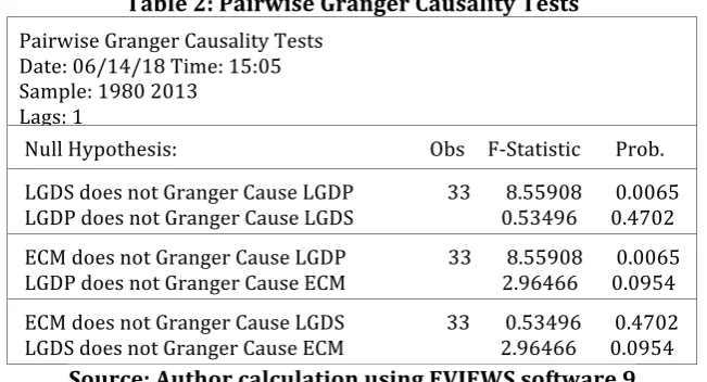
Table 2: Pairwise Granger Causality Tests

Pairwise Granger Causality Tests Date: 06/14/18 Time: 15:05 Sample: 1980 2013

Lags: 1

Null Hypothesis: Obs F-Statistic Prob.

LGDS does not Granger Cause LGDP 33 8.55908 0.0065 LGDP does not Granger Cause LGDS 0.53496 0.4702 ECM does not Granger Cause LGDP 33 8.55908 0.0065 LGDP does not Granger Cause ECM 2.96466 0.0954 ECM does not Granger Cause LGDS 33 0.53496 0.4702 LGDS does not Granger Cause ECM 2.96466 0.0954

Source: Author calculation using EVIEWS software 9

Selection Of Lag Length

A general model of ARDL is first performed with the lag length to select the lag length of the VAR model the selection criteria is used, Sequential Modified Likelihood Ratio (LR), Final Prediction Error (FPE), Akaike Information Criterion (AIC), Schwarz Information Criterion (SIC) and Hannan-Quinn Information Criterion (HQ) are employed. It is clear from Table 3 that LR, FPE, AIC, SC, HQ and HQ statistics have chosen lag 1for each endogenous variable in their autoregressive and distributed lag structures in the estimable VAR model. Therefore, lag of 1 is used for estimation purposes.

Table 3:: VAR Lag Order Selection Criteria

VAR Lag Order Selection Criteria Endogenous variables: LGDP LGDS Exogenous variables: C

Sample: 1980 2013 Included observations: 31

Lag LogL LR FPE AIC SC HQ

0 -19.33021 NA 0.013574 1.376143 1.468658 1.406300

1 51.76152 128.4238* 0.000179* -2.952356* -2.674810* -2.861883*

2 54.07715 3.884288 0.000201 -2.843687 -2.381111 -2.692899

3 58.63988 7.064867 0.000196 -2.879992 -2.232385 -2.668888

* indicates lag order selected by the criterion

LR: sequential modified LR test statistic (each test at 5% level) FPE: Final prediction error

AIC: Akaike information criterion SC: Schwarz information criterion HQ: Hannan-Quinn information criterion

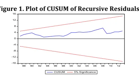
VECM Stability Test

(8)

CUSUM and CUSUM of squares for equation 1

Figure 1. Plot of CUSUM of Recursive Residuals

-16 -12 -8 -4 0 4 8 12 16

88 90 92 94 96 98 00 02 04 06 08 10 12

CUSUM 5% Significance

Figure 2. Plot of Cumulative Sum of Squares of Recursive Residuals

-0.4 -0.2 0.0 0.2 0.4 0.6 0.8 1.0 1.2 1.4

88 90 92 94 96 98 00 02 04 06 08 10 12

CUSUM of Squares 5% Significance

Note: The straight lines represent critical bounds at 5% significance level.

In order to establish the validity of the estimates, a number of diagnostic tests including the Jarque-Bera normality test statistics of 34.9506 with the probability value of (0.0000), the Breusch-Godfrey serial correlation LM test statistics of 1.996219 with the probability value of (0.1309 and ARCH test for heteroscedasticity of 0.004547 with the probability value of (0.9444)are carried out.

Overall, the Results indicate the soundness of the equations; correct specification of the model and the absence of serial correlation and heteroscedasticity, but the residuals are not normally distributed, and this is the only problem in our model. To determine the stability of the parameters of the estimated equation, the CUSUM and CUSUM of squares test is carried out. From the results the model is stable. The next step is to ascertain the presence of a long run relationship amongst the variables. To do this we employ the bounds test, the results of which are presented in the table 4 below:

Table 4: Bounds Test Results

Dependent variable Function F-Statistic

DLGDP α + DLGDP, DLGDS 5.385579**

DLGDS DL DGDS, DLGDP 3.175314

Asymptotic critical value Significance Level 5% 10%

Lower bound 4.94* 4.04**

Upper bound 5.73* 4.78**

Notes: DLGDP is the first difference lag of GDP and DLGDS is the first difference lag of GDS. The critical values for the lower I (0) and upper I (1) bounds are taken from Pesaran et al. (2001), Appendix: Table CI (iii) Case III: (unrestricted intercept and no trend)). *, ** Significant at 5% and 10% significance levels, respectively

(9)

are given in Table 3. Based on Table 4 above, the results suggest the existence of cointegration, when LGDP is the dependent variable as the computed F= 5.85579is greater than the upper bound critical value at 10% level. Meaning that we can reject HN and accept HA, meaning that the two variables DLGDP and DLGDS have long run association ship over the period of 1980-2013 in UAE. However, there is no evidence of cointegration when DLGDS is taken as dependent variable as the computed F= 3.175314 is lower than the lower bound critical value at 5% level. In other words, these results suggest that DLGDS and DLGDP have no long run association ship when LGDS is a dependent variable. These results is consistent with the findings of (Mphuka,2010)[21], (Abu Al-Foul,2010) [9], (Nurudeen,2010) [22] and (Mohan,2006) 25].The next stage of the procedure would be to estimate the coefficients of the long-run relations and the associated error correction model (ECM) using the ARDL approach. The appropriate lags on variables is automatically selected using Schwartz Bayesian Criterion (SBC) these tests, and turned out to be the ARDL (2, 3). The long-run estimated coefficients are shown in the Table 5. The results show that LGDS does not contribute to economic growth significantly. It is concluded based on our findings that the coefficient of LGDS positive and statistically not significant, meaning that if LGDS increase or decrease by 1 percent LGDP increase (decreases) economic growth just by 24.11 percent. Indeed, the size of coefficient is big and insignificant. The effect of LGDS in difference one period on economic growth is positive and statistically significant at 5 percent and 1 per cent increase in LGDS on economic growth contributes economic growth by 30.41 percent.

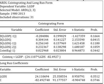
Table 5: Short-run and long-run relationships

ARDL Cointegrating And Long Run Form Dependent Variable: LGDP

Selected Model: ARDL(2, 3) Sample: 1980 2013

Included observations: 31

Cointegrating Form

Variable Coefficient Std. Error t-Statistic Prob.

D(LGDP(-1)) -0.284086 0.199029 -1.427359 0.1664

D(LGDS) 0.304144 0.141227 2.153590 0.0415

D(LGDS(-1)) 0.256140 0.157969 1.621458 0.1180

D(LGDS(-2)) 0.232367 0.138298 1.680187 0.1059

CointEq(-1) 0.022968 0.023804 0.964873 0.3442

Cointeq = LGDP - (24.1107*LGDS -82.4927 )

Long Run Coefficients

LGDS 24.110694 25.358554 0.950791 0.3512

(10)

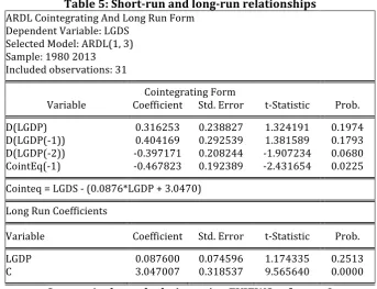
Table 5: Short-run and long-run relationships

ARDL Cointegrating And Long Run Form Dependent Variable: LGDS

Selected Model: ARDL(1, 3) Sample: 1980 2013

Included observations: 31

Cointegrating Form

D(LGDP) 0.316253 0.238827 1.324191 0.1974

D(LGDP(-1)) 0.404169 0.292539 1.381589 0.1793

D(LGDP(-2)) -0.397171 0.208244 -1.907234 0.0680

CointEq(-1) -0.467823 0.192389 -2.431654 0.0225

Cointeq = LGDS - (0.0876*LGDP + 3.0470)

Long Run Coefficients

LGDP 0.087600 0.074596 1.174335 0.2513

C 3.047007 0.318537 9.565640 0.0000

Table 6 shows that the result of ECM of selected ARDL (2,3) When LGDP as a dependent variable the ECM (-1) = 0.02296 (positive) and P-value=0.3442 greater than 0.05, meaning that there is no SR association ship. The coefficients of ECM terms present the speed of adjustment in the long-run due to a shock is not effective. The results of ECM of selected ARDL (1,3) were analyzed in Table 6. The estimated value of error correction coefficient was -0. 467823; which was significant at p=0.0225 and showed negative sign. It established the association between LGDS and independent variables of LGDP. The calculated value of ECM recommended the rate of amendment of the long-term disequilibrium due to short-term interruption of the preceding year.

CONCLUSION AND POLICY IMPLICATIONS

(11)

effective. While, there is negative (-0.467823) and significant error correction term (0.0225) which less than 5 percent level of significance. Which implies the adjustment process to restore equilibrium in the long run by 46.78 percent. While the result of ECM of selected ARDL (2,3) When LGDP as a dependent variable the ECM (-1) = 0.02296 (positive) and P-value=0.3442 greater than 0.05, meaning that there is no SR association ship. The coefficients of ECM terms present the speed of adjustment in the long-run due to a shock is not effective. Considering the findings mentioned above, we make the following recommendations; Measures to increase growth and economic diversification in UAE should aim to promotes domestic savings and increases domestic savings overall. Fiscal and Monetary policies that allow for increased savings and that enhances domestic savings is vital. The study recommends the need for development of financial instruments to encourage domestic savings. Moreover, if domestic savings are invested efficiently and are therefore an important factor of economic growth, the main objective of national economic policy should be to encourage the people to save. In addition, national economic authorities should create appropriate conditions for the reallocation of national resources from traditional (non-growth) sectors to the so-called modern (growth-led) sectors of the economy.

The present study like the existing studies on the debate, therefore, suggests that the relationship between LGDP and LGDS is country-specific even among the fastest growing economies. Each country should, therefore, set up policies individually to achieve either of the macroeconomic variables. However, the existence of a long- run relationship between the variables is general among the countries.

References

Harrod, R. F. (1939). An Essay in Dynamic Theory. Economic Journal. XLIX, 14-33.

Domer, E. (1946). Capital Expansion, Rate of Profit and Employment. Econometrica, 14(2), 137-147.

Solow, R. M. (1956).A Contribution to the Theory of Economic Growth. Quarterly Journal of Economics, 70, 65-94.

Lean, H. H. & Song, Y.(2009).The Domestic Savings and Economic Growth Relationship in China. Journal of Chinese economic and Foreign Trade Studies, 2, (1), 5-17.

Sheggu, D.(2009).Causal Relationship between Growth and Real Gross Domestic Savings: Evidence from Ethiopia. Sinha, D. & Sinha, T. (1998).Cart before the Horse? The Saving-Growth Nexus in Mexico. Economics Letters, 61, 43-47

Saltz, I. S. (1999).An Examination of the Causal Relationship between Savings and Growth in the Third World. Journal of Economics and Finance, 23(1), 90-98.

Anoruo, E. & Ahmad, Y. (2001). Causal Relationship between Domestic Savings and Economic Growth: Evidence from Seven African Countries. African Development Bank, 13(2), 238-249.

Abu, N.(2010). Saving —Economic Growth Nexus in Nigeria, 1970-2007: Granger Causality and Cointegration Analyses, Review of Economic & Business Studies, Vol. 3, p. 93-104.

Masih, L., & Peters, M. (2010). A revisitation of the savings–growth nexus in Mexico. Economics Letters, 107(2010), 318–320.

Tang, C. F., & Tan, B. E. (2014). A revalidation of the savings–growth nexus in Pakistan. Economic Modeling, 36(2), 370–377.

Alguacil, M., Cuadros, A., & Orts, V. (2004). Does saving really matter for growth? Mexico (1970–2000). Journal of International Development, 16(2), 281–290.

Anoruo, E., & Ahmad, Y. (2001). Causal Relationship between domestic savings and economic growth: Evidence from seven African countries. African Development Bank, 13(2), 238–249.

(12)

Zeren, F. & Ekrem, A. Y. (2013). Empirical Analysis of the Savings-Growth Nexus in Turkey. Journal of Business, Economics and Finance, 2(3), 352–367.

Persaran, H.M., Shin, Y and Smith, J. (2001), Bound Testing Approaches to the Analysis of Level Relationships‟ Journal of Applied Econometrics.

Adeleke, A. M.(2014). Saving-Growth Nexus in an Oil-Rich Exporting Country: A Case of Nigeria. Management science and Engineering. http://www. cscanada. net/index.php/ mse/ article/view/5417

Robson Mandishekwa..(2014).Causality between Economic Growth and Investment in Zimbabwe. Journal of Economics and Sustainable Development. Vol.5, No.20,136.

Samantraya, A. and Patra, S.K., 2014. Determinants of Household Savings in India: An Empirical Analysis Using ARDL Approach, Economics Research International, No. 454675.

Jangili, R. (2011). Causal Relationship between Saving, Investment and Economic Growth for India-Does the Relation Imply (Munich Personal RePec Archive (MPRA), Paper 40002). Germany:University Library of Munich. Google Scholar

Mphuka. C, (2010). Are Savings Working for Zambia's Growth? Zambia Social Science Journal, Vol 1.No2 ,Article 6.

Nurudeen, Abu.(2010).Saving-Economic Growth Nexus in Nigeria, 1970-2007: GrangerCausality and Co-Integration Analyses. Review of Economic and Business Studies. 3(1).

Dipendra, S. (2009). "Saving and Economic Growth in India", Munich Personal RePEcArchive,Vol. 199, p. 1-18.

Hemmi, N. et al.(2007).The Long-Term Care Problem, Precautionary Saving, andEconomic Growth.Journal of Macroeconomics, Vol 29, p. 60—74. Inder, B. (1993)

Mohan, R. (2006). Causal Relationship between Savings and Economic Growth in Countries with Different Income levels. Economics Bulletin, 5(3), 1-12.

Sheggu, D. (2009). Causal Relationship between Growth and Real Gross Domestic Savings: Evidence from Ethiopia World Bank Development Indicators (World Bank, 2014),online.

Engle, R.F.,and Granger, C.J. 1987. “Cointegration and Error-correction - Representation, Estimation, and Testing”, Econometrica 55, 251-78.

Johansen, S. (1988), “Statistical Analysis of Cointegration vectors”, Journal of Economic Dynamics and Control, 12, pp.231-54

Johansen, S.,and Juselius, K. 1990. “Maximum likelihood estimation and inference on cointegration-with application to the demand for money”. Oxford bulletin of economics and statistics, 52: 169-210.

Pesaran, M.H. and Y. Shin (1995). "An Autoregressive Distributed Lag Modeling Approach to Co-Integration Analysis,"Cambridge University, p. 134-150.

Pesaran, M.H., and Y. Shin (1996). "Co-Integration and Speed of Convergence to Equilibrium," Journal of Econometrics, Vol 71, p. 43-117.

Pesaran, H.M. and Shin, Y. (1999), An Autoregressive Distributed Lag Modeling Approach to Cointegration Analysis, in storm, S. (Ed), Econometrics and Economic Theory in the 20th century, the ranger Frish Centennial symposium, Cambridge University Press