Investigation On Various Training Algorithms For Robust ANN-PID Controller Design

5352

Investigation on Various Training Algorithms for

Robust ANN-PID Controller Design

Abstract : The classical off-line tuning of PID controller may not cope-up with the real-time disturbances as the control design process is independent of disturbance characteristics. So, the recent research focuses on making this tuning process on-line by using artificial intelligence techniques. Among various artificial intelligence/machine learning techniques, neural networks (NN) provide multiple features such as control design, forecasting, regression analysis, etc. However, the efficacy of artificial NN depends on how well the system is getting trained. Besides, there are many training algorithms available for implementing artificial NN to tune PID controller gain parameters for a given system. However, the selection of suitable training algorithm influences the effectiveness of the PID controller in the system. Moreover, the effective algorithm identified for one system may not work well for another type of system. So, it is always an important task to analyze which algorithm works better for the given system characteristics. With this intent, this paper presents a quantitative investigation on implementation procedure and response characteristic of different typical artificial NN training algorithms when applied to tune PID controller gain values to provide a robust control action for a considered system. The analysis has been presented with the help of MATLAB/Simulink® based simulation results.

Index Terms : Artificial Neural Network, Bayesian Regularization, Levenberg-Marquardt Algorithm, PID tuning, Scaled Conjugate Gradient. ——————————  ——————————

1.

INTRODUCTION

In THE conventional process of PID tuning, the robustness of the controller depends on picking the suitable tuning method because an identified effective method for one system may not be effective for all other systems [1], [2]. Also, in the conventional approach, the tuned PID controller may not cope-up with the disturbances that arise when the system is running [3], [4]. So, there is a need for moving to the online tuning methods, such as artificial NN based control, which can tune the controller according to the real-time disturbances by using artificial intelligence [5], [6]. However, in the artificial NN, the efficiency of tuning depends on the algorithm that is being used for training the NN [7]. Artificial NN has been used in different systems, moreover, the effective algorithm for one system may not be effective for other systems. For example, levenberg-marquardt algorithm has been used in finding the gear fault diagnosis [8], estimation of seismic response [9], temperature control process [10], etc. Bayesian regularization algorithm has been used in semiconductor processing [11], measuring uncertainty in wearable sensors [12], predicting oil gas drilling cost [13], etc.

Similarly, scaled conjugate algorithm has been used in hand gesture control of robotic arm [14], assessment of electromagnetic compatibility [15], etc. In all these cases, the algorithm for tuning artificial NN is taken in random but the problem here is that the chosen algorithm mayn‘t be the efficient algorithm. So, the suitability of each and every algorithm should be checked to pick the best one. With this motivation, there were some evaluations available in the literature for selecting the better suitable algorithm for various applications, for e.g., in SOC performance estimation [16], object detection [17], solving knight‘s tours [18], etc. Hence, type of NN architecture and selection of training algorithm is a very important task. However, from the abovementioned literature, it was understood that these attempts were very limited against the wide applications of artificial NN, especially for control engineering application. There are no such approaches available for finding the best training algorithm for control applications. So, to address this issue, this paper provides a comprehensive investigation to analyze the impact of different typical NN training algorithms for tuning the PID controller and suggests best algorithm for PID tuning. The analysis is carried out by considering a real-time application, named, liquid level system (LLS) [19].

2.

ARTIFICIAL

NEURAL

NETWORK

ARCHITECTURE

Artificial NN consists of a number of highly interconnected information processing elements. The revolutionary work of McCulloch and Pitts was the foundation for the growth of different architectures of NNs, such as, single-layer feed forward NN, multi-layer feed forward NN, and recurrent or feedback NN that are explained as given below.

2.1 Single Layer Feed Forward Network

A feed forward network that consists of two layers, named, input layer and output layer is called single layer feed forward neural network. In general, we don‘t count the input layer as a separate layer, because it doesn‘t compute and just act as fan out device passing the signal from other neurons. Hence, this network is called single-layer network. The input neurons of network receive the inputs and the output neurons send the output signals. The synaptic junctions connect each neuron of

____________________________________

 Mr. K. Sandeep Rao is pursuing B.Tech in Electronics and Communication Engineering at School of Electronics Engineering, Vellore Institute of Technology - Andhra Pradesh (VIT-AP) University, Amaravati-522237, Andhra Pradesh, INDIA, E-mail: [email protected]

 Mr. V. N. Siva Praneeth is pursuing B.Tech in Electronics and Communication Engineering with Specialisation in VLSI at School of Electronics Engineering, Vellore Institute of Technology - Andhra Pradesh (VIT-AP) University, Amaravati-522237, Andhra Pradesh, INDIA, E-mail: [email protected]

 Dr. Y. V. Pavan Kumar is working as an Associate Professor in School of Electronics Engineering, Vellore Institute of Technology - Andhra Pradesh (VIT-AP) University, Amaravati-522237, Andhra Pradesh, INDIA, Tel: +91863-2370155. E-mail: [email protected]

5353

input layer with all the neurons of the output layer so that the input signal is transmitted to the output, but not vice-versa. Such networks are called feed forward networks. Fig. 1 shows the single layer feed forward NN, where x1, x2…xp are the

input signals, y1, y2…yn are the output signals, and ‗Wjk‘ are

the weights connected between the neurons from input layer to all the neurons in output layer. A single-layer non-linear feed forward network can‘t realize XOR function. This is addressed by increasing the number of layers of the network. So, a multilayer network with non-linear activation function has evolved, which can realize any non-linear function like XOR.

x

₁

x

₂

x

_p

y

₁

y

₂

y

_n

W

k

_j

Fig. 1. Architecture of single-layer feed forward network.

2.2 Multi-layer Feed Forward Neural Networks

A multi-layer feed forward network consists more number of layers with one input layer, one output layer, and one or more intermediate layers, called hidden layers. The processing units in the hidden layers are called hidden neurons. Hidden layers do the intermediate computations before propagating the inputs to target layers. The connecting weights that are linked between input layer to hidden layer are called input-hidden layer weights (Wjk), and the connecting weights linked

between hidden layer to output layer are called hidden-output layer weights (Wij). A multi-layer feed forward network with ‗p‘

number of input neurons, ‗m‘ number of hidden neurons and ‗n‘ number of output neurons is called as ‗l-m-n‘ architecture which is shown in Fig. 2. The connections in the architecture are allowed from one layer to its succeeding layer but not to its preceding layer. The hidden layer gets the information from input layer and processes the output to the next hidden layer or output layer after computing internally.

x

₁

x

₂

x

_p

y

₁

y

₂

y

_n

k

j

i

W

W

_v

₁

v

₂

v

_m

Fig. 2. Multi-layer feed forward network.

2.3 Recurrent Neural Networks

These are the neural networks in which there is an at least one feedback loop. The feedback loop may be the link from one of the neurons from output layer to neuron in hidden layer or self-feedback of neuron which means the output of a neuron is fed back to itself as an input. This is shown in Fig. 3. The TABLE 1 gives the brief comparison of feed forward and recurrent neural networks.

x

₁

x

₂

x

_p

y

₁

y

₂

y

_n

W

W

Self-feedback

Feedback Path

Self-feedback

j

_i

k

v

₁

v

₂

v

_m

Fig. 3. Recurrent neural network

TABLE 1: Comparison of feedforward and recurrent NNs

S. No Feed forward NNs Recurrent NNs 1 Solutions are known Solutions are unknown 2 Weights are learned Weights are arranged 3 Evolves in the ―weight _space‖ Evolves in the ―state _space‖

4

Used for - Prediction - Classification - Functional

approximation

Used for

- Constraint satisfaction - Optimization

- Feature matching

3.

WEIGHT

UPDATING

ALGORITHMS

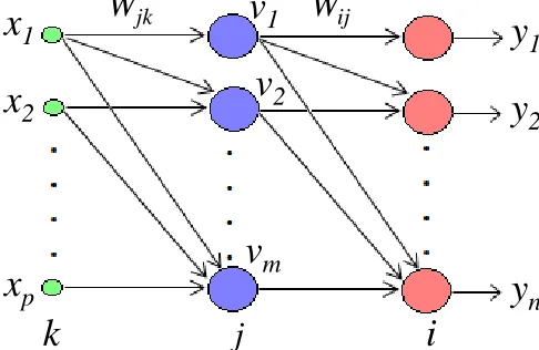
3.1 Levenberg-Marquardt (LM) Algorithm

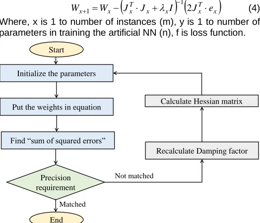
Levenberg Marquardt Algorithm (LMA) is one of the algorithms of the least square algorithms [20], [21]. It is generally called Damped Least Square Method [22]. It was discovered by Kenneth Levenberg and Donald Marquardt and this algorithm is coined with their names. It is the most generally used algorithm for optimization. It is the common way for solving the nonlinear systems [23]. It is more suitable for small and medium sized systems in artificial NN [24]. The weight updating rule used for LMA is given by (1). The flow of operations is given in Fig. 4. LMA has stable convergence. The main application of LMA is curve fitting problems.

d I H W

5354

minimum is not global minimum in all cases. The hessian matrix is computed by computing Jacobian matrix and the gradient vector as given by (2) and (3) respectively. Thus, the approximated hessian matrix is given by (4).

y x y x W E J    , (2) I J J

Hf 2 T   (3)



 



T x x x T x x

x W J J I J e

W _1    12  (4) Where, x is 1 to number of instances (m), y is 1 to number of parameters in training the artificial NN (n), f is loss function.

Start

Initialize the parameters

Precision requirement Put the weights in equation

Find “sum of squared errors”

Calculate Hessian matrix

Recalculate Damping factor

End

Not matched

Matched

Fig. 4. Flow chart used in levenberg marquardt algorithm

Based on the bending factor (λ) value, different cases can be realized as given follows.

 Case 1 - when λ is zero: the LMA becomes equivalent to newton method by using the approximated hessian matrix.

 Case 2 - when λ is too large: the LMA becomes equivalent to gradient descent method, which uses smaller training states.

3.2 Bayesian Regularization (BR) Algorithm

Bayesian Regulation (BR) algorithm is derived based on ―Bayes theorem‖ and is more efficient than the standard back propagation methods [25], [26]. During the BR process, the nonlinear regression relations are converted to second order linear regression based mathematical equations. The main challenge lies in selection of the absolute fitting values for the function parameters. In artificial NN, the BR framework works by the probabilistic interpretation of given network parameters, which varies it from traditional training methods, where, set of weights are chosen by minimization of error function. But, in BR algorithm, a performance function given by (5) is used to find the error, i.e., difference between actual and predicted data during the process of training. In a BR algorithm, regularization adds an extra term and function in order to obtain smooth mapping, which uses a gradient-based optimization for minimizing the objective and performance function as given in (6). Once the data is taken for training, to address the additional noise present in the targets, posterior distribution of weights of the NN will be updated as required.





_





t y x

N A w T S F P 1 2 1 , . (5)





 

S F

P.  t ,  m (6)

Where, St denotes the sum of the squares of network error

values, T is the input and target pairs of training set, A is NN architecture that contains information about number of layers and number of units in each layer, Sm is sum of squares of

the network weights, (w, λ, µ) are the specifications that are required to estimate parameters of the function, μSm(w|A) is

the weight decay, μ is the rate of decay (If μ << λ, then the algorithm will minimize errors. if μ >> λ, then the network will produce a smooth response).

3.3 Scaled Conjugate Gradient (SCG) Algorithm

Scaled conjugate methods were developed by Magnus Hestenes and Eduard Stiefel. These methods use the linear search in each iteration. These are mainly used for solving the linear systems. There are many sub-methods in conjugate gradient methods [27]. SCG algorithm is one of those sub-methods [28]. The applications of the SCG algorithm are constrained optimization, curve fitting, etc. It works with feedforward artificial NNs. These methods solve, when all the errors are in the region of assumed values [29]. The main part of the conjugate methods is the calculation of the direction of the weights, which is practically difficult. The flow of operations of the SCG algorithm is given in Fig.5. The training data function and the parameter vector function are given by (7) and (8) respectively. The key limitation of SCG algorithm is, it won‘t provide any data related to the calculation and inversion of the hessian matrix [30].



 



x G S

S _1 _1   (7)

  

 



1   

 W S for x

Wx x x x (8)

Where, γ is SCG parameter, S0 = -G0 is initial direction vector,

η is training rate, and W0 is the initial parameter vector.

Start

Initialize the parameters

Precision requirement Put the weights in equation

Calculate the “training rate”

Recalculate Gradient training direction

End

Not matched

Matched

Fig. 5. Flow chart used in conjugate gradient algorithm

4.

PERFORMANCE

ANALYSIS

&

CASE

STUDY

5355

mean square error (RMSE), which are useful to understand the performance of the training algorithms. The relations for MSE, MBE, RMSE and error (%) are given from (9) to (11).



















Error (12)

Where, Tx is target value, Ox is output value, N is number of

patterns that are used. Regression plot analysis is another method used to know the performance of the training algorithm and is drawn between the target value and the output value. Regression plot gives the brief information of how the data is scattered. The correlation coefficient (R) is the measure of correlation between the outputs and targets w.r.t validation, training, and test data sets. The line in regression plot will be in 450 to x-axis and for R = 1 is where output of network is equal to target value. The value of R is 1, if there exists a close relation between targets to outputs. Error histogram is an another indicative of the performance of the trained NN. It is a plot drawn between the error value and the number of instances that a particular value occurs. The bars present in the plot represent the number of instances that a particular error occur. It gives the information about the points, where the data is significantly worse than any other. This paper took a liquid level system (LLS) application with an objective of maintaining the water level as constant. The transfer function of single tank LLS [19] is given by (13).

s e s s

G 8.415

1 826 . 12 315 . 0 ) (    (13)

In this work, the liquid level of the tank is controlled by a PID controller, whose KP, KI and KD values are estimated by the

artificial NN. Three training methods LM, BR, SCG are used to train the artificial NN. The efficacy of these methods is analyzed using MATLAB/Simulink simulations. The model used to control liquid level system is given in Fig. 6.

1 826 . 12 315 . 0  s 1 826 . 12 315 . 0  s 1 826 . 12 315 . 0  s

Fig. 6. Artificial NN – PID model designed with different

training algorithms to control LLS

5.

RESULTS

AND

DISCUSSION

The considered case study, i.e., LLS control is subjected to step input and the response of the system for different PID control parameters that are trained with artificial NN is presented. The effectiveness of the LM, BR and SCG training algorithms for PID tuning are evaluated in three modes, such as analysis through training performance plots, analysis through time domain transient response plots, and analysis through stability plots as given follows.

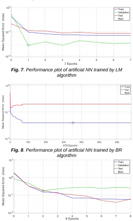
5.1 Analysis Through Training Performance Plots

The plots pertaining to training performance of LM, BR and SCG algorithms are shown in Fig. 7, Fig. 8, and Fig. 9

respectively. The performance of a neural network is said to be satisfied if the error value reduces for every epoch and the best validation performance value should be minimum.

Fig. 7. Performance plot of artificial NN trained by LM algorithm

Fig. 8. Performance plot of artificial NN trained by BR algorithm

Fig. 9. Performance plot of artificial NN trained by SCG algorithm

5356

The regression plots for the three training methods for different values of regression coefficients are plotted in Fig. 10, Fig. 11, and Fig. 12 respectively. The values of regression coefficient computed during training phase, testing phase, and the overall phase for all the three artificial NN training methods, and is given in TABLE 2.

Fig. 10. Regression plot of artificial NN trained by LM algorithm

Fig. 11. Regression plot of artificial NN trained by BR

algorithm

Fig. 12. Regression plot of artificial NN trained by SCG algorithm

TABLE 2: Regression coefficients for NN training methods.

Algorithm Training Regression

Testing Regression

Total Regression

LM 0.98572 0.98572 0.98602

BR 0.99332 0.95248 0.98881

SCG 0.98504 0.99399 0.98552

Fig. 13. Error histogram of artificial NN trained by LM algorithm

5357

Error histogram plots are plotted between the error and the instances. The error histogram plots for data trained using LM, BR and SCG algorithms are given in Fig. 13, Fig. 14 and Fig. 15 respectively. If maximum number of instances have less error, then the training performance of that particular algorithm is good. The plots indicate that artificial NN trained using BR algorithm gives least error for maximum samples.

Fig. 15. Error histogram of artificial NN trained by SCG algorithm

To understand the training failures, training state plots are drawn for different algorithms as shown in Fig. 16, Fig. 17 and

Fig. 18. From these plots, it is observed that BR algorithm gives minimum number of failures among other algorithms. Another metric to assess the performance of the training algorithms is plot fit, which is performed by plotting the output and the target for all the samples. The plot fit diagrams are given in Fig. 19, Fig. 20 and Fig. 21 respectively. The observation of these plots indicate that the BR algorithm gives better performance in terms of the error estimated by plot fits.

Fig. 16. Training state of artificial NN trained by LM algorithm

Fig. 17. Training state of artificial NN trained by BR algorithm

Fig. 18. Training state of artificial NN trained by SCG algorithm

Fig. 19. Plot fit of artificial NN trained by LM algorithm

Fig. 20. Plot fit of artificial NN trained by BR algorithm

Fig. 21. Plot fit of artificial NN trained by SCG algorithm

5.2 Analysis Through Time Domain Transient Plots

The transient analysis of the LLS is performed by feeding step signal as input. The KP, KI and KD coefficients of the PID

controller are computed using three different artificial NN training algorithms, viz., LM, BR, and SGC. The performance is examined and given in Fig. 22, Fig. 23 and Fig. 24. The comparative analysis of all the step responses is presented in

5358

respect to the transient response performance index such as; percentage maximum peak overshoot (Mp), delay time (td),

rise time (tr) and settling time (ts) is given in TABLE 3.

Fig. 22. Time response with artificial NN-PID using LM algorithm

Fig. 23. Time response with artificial NN-PID using BR algorithm

Fig. 24. Time response with artificial NN-PID by SCG algorithm

Fig. 25. Cumulative result obtained by artificial NN-PID

TABLE 3: Time domain parameters computed for step input

Algorithm Mp (%) td tr ts

LM 15 16.81 30.17 179.95

BR 0 16.47 14.02 60.75

SCG 0 16.96 16.71 75.6

From the results deposited in Fig.25 and TABLE 3, it is observed that the LM algorithm gives highest peak overshoot where as other two methods show zero overshoot. The delay time computed with all the three algorithms are almost comparable, whereas, BR algorithm of training artificial NN offers lesser rise time and settling time compared to other two algorithms. Hence, it is concluded that artificial NN trained using BR algorithm provide satisfactory performance with respect to the transient time domain performance indices.

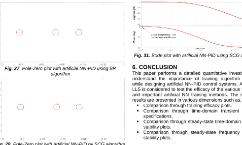
5.3 Analysis Through Stability Response Plots

To understand the dynamics of the system in closed loop, the poles and zeroes of the system with PID controller in feedback are plotted and examined. Three pole-zero plots, one for each method of training the artificial NN are plotted as given in Fig. 26, Fig. 27 and Fig. 28. The analysis shows that the placement of poles and zeroes for all the plots are different. The bode plots are also plotted as given in Fig. 29, Fig. 30

and Fig. 31. All these plots are helpful in identifying the most stable response and its associated training method. From these plots, the following comments could be made.

 From Fig. 26, i.e., the response obtained by LM algorithm, it can be seen that all poles are lying on the left-side of s-plane. So, the system is ―stable‖.

 From Fig. 27, i.e., the response obtained by BR algorithm, it can be seen that all poles are lying on the left-side of s-plane. Further, these poles are located at far ends of left-side when compared to Fig. 26. So, the system is relatively ―more stable‖ when compared to Fig. 26.

 From Fig. 28, i.e., the response obtained by SCG algorithm, it can be seen that this plot is also having similar nature of the response obtained with BR algorithm, i.e., Fig. 27. So, the system is ―stable‖.

5359

Fig. 27. Pole-Zero plot with artificial NN-PID using BR algorithm

Fig. 28. Pole-Zero plot with artificial NN-PID by SCG algorithm

From the frequency response stability plots, i.e., bode plots given through Fig. 29, Fig. 30 and Fig. 31, the phase margin and gain margin for the LLS control system is computed. From these values, it is observed that the system is ―more stable‖ with BR algorithm and SCG algorithm when compared to LM algorithm.

Fig. 29. Bode plot with artificial NN-PID using LM algorithm

Fig. 30. Bode plot with artificial NN-PID using BR algorithm

Fig. 31. Bode plot with artificial NN-PID using SCG algorithm

6.

CONCLUSION

This paper performs a detailed quantitative investigation to understand the importance of training algorithm selection while designing artificial NN-PID control systems. A practical LLS is considered to test the efficacy of the various traditional and important artificial NN training methods. The respective results are presented in various dimensions such as,

 Comparison through training efficacy plots.

 Comparison through time-domain transient response specifications.

 Comparison through steady-state time-domain response stability plots.

 Comparison through steady-state frequency response stability plots.

These comparative results and analysis confirms that the selection of proper artificial NN training algorithm critically influences the stability, error performance, and the response of the system. Finally, out of this investigation, it is identified as the BR algorithm provides comparatively better response on LM and SCG algorithms.

7

REFERENCES

[1] Rosmin Jacob, Senthil Murugan, ―Implementation of neural network based PID controller,‖ International Conference on Electrical, Electronics, and Optimization Techniques (ICEEOT), 2016.

[2] Ran Wang, Zhicheng Zhou, Guangji Qu, ―Fuzzy neural network PID control based on RBF neural network for variable configuration spacecraft,‖ IEEE 3rd Advanced Information Technology, Electronic and Automation Control Conference (IAEAC), 2018.

[3] Chathura Wanigasekara, Dhafer Almakhles, Akshya Swain, Sing Kiong Nguang, Umashankar Subramaniyan, Sanjeevi kumar Padmanaban, ―Performance of neural network based controllers and ΔΣ-based PID controllers for networked control systems: a comparative investigation,‖ IEEE International Conference on Environment and Electrical Engineering and IEEE Industrial and Commercial Power Systems Europe (EEEIC / I&CPS Europe), 2019.

[4] Xiong Jingjing, Liu Jiaoyu, ―Neural network PID controller auto-tuning design and application,‖ 25th

Chinese Control and Decision Conference (CCDC), 2013.

5360 [6] Yu Yongquan, H. Ying, Z. Bi, ―A PID neural network

controller,‖ Proceedings of the International Joint Conference on Neural Networks, 2003.

[7] D. Fourer, G. Peeters, ―Fast and adaptive blind audio

source separation using recursive levenberg-marquardt synchrosqueezing, IEEE International Conference on Acoustics, Speech & Signal Processing (ICASSP), 2018.

[8] Tang Jia-li, Liu Yi-jun, Wu Fang-sheng, ―Levenberg-Marquardt neural network for gear fault diagnosis,‖ International Conference on Networking and Digital Society, 2010.

[9] R. Sarem, A. J. Rahimi, S. Varadharajan, ―Estimation

of seismic response of mass irregular building frames using artificial intelligence,‖ 9th International Conference on Cloud Computing, Data Science & Engineering, 2019.

[10] N. Patil, D. R. Patil, ―Implementation of artificial neural

network on temperature control process,‖ 2nd

International Conference on Intelligent Computing and Control Systems (ICICCS), 2018.

[11] C. H. Chen, P. Parashar, C. Akbar, S. Ming Fu, M. Y. Syu, A. Lin, ―Physics-prior bayesian neural networks in semiconductor processing,‖ IEEE Access, Vol. 7, pp. 130168 – 130179, 2019.

[12] Ali Akbari, Roozbeh Jafari, ―A deep learning assisted

method for measuring uncertainty in activity recognition with wearable sensors,‖ IEEE EMBS International Conference on Biomedical & Health Informatics (BHI), 2019.

[13] Z. Yue, Z. S. Zheng, L. Tianshi, ―Bayesian regularization bp neural network model for predicting oil-gas drilling cost,‖ International Conference on Business Management and Electronic Information, 2011.

[14] B. Schabron, Z. Alashqar, N. Fuhrman, K. Jibbe, J. Desai, ―Artificial neural network to detect human hand gestures for a robotic arm control,‖ 41st

Annual International Conference of the IEEE Engineering in Medicine and Biology Society (EMBC), 2019.

[15] C. B. Khadse, M. A. Chaudhari, V. B. Borghate, ―Electromagnetic compatibility estimator using scaled conjugate gradient backpropagation based artificial neural network,‖ IEEE Transactions on Industrial Informatics, Vol. 13, No. 3, pp. 1036-1045, June 2017.

[16] W. Jian, X. Jiang, J. Zhang, Z. Xiang, Y. Jian, ―Comparison of SOC estimation performance with different training functions using neural network,‖ 14th

International Conference on Modelling and Simulation, 2012.

[17] S. Kim, Seong-heum Kim, Y. Hwang, J. Jeong, ―Comparison of training methods for the binarized neural object detection network,‖ 34th

International Technical Conference on Circuits/Systems, Computers and Communications (ITC-CSCC), 2019.

[18] R. G. Escalante, H. A. Malki, ―Comparison of artificial

neural network architectures and training algorithms for solving the knight‘s tours,‖ IEEE International Joint Conference on Neural Network Proceedings, 2006.

[19] B. V. Murthy, Y. V. P. Kumar, V. R. Kumari, ―Application of neural networks in process control: automatic online tuning of PID controller gains for

±10% disturbance rejection,‖ 2012 IEEE International Conference on Advanced Communication Control and Computing Technologies (ICACCCT), 2012.

[20] J. Hao, G. Zhang, Y. Zheng, W. Hu, K. Yang, ―Solution

for selective harmonic elimination in asymmetric multilevel inverter based on stochastic configuration network and levenberg marquardt algorithm,‖ IEEE Applied Power Electronics Conference and Exposition (APEC), 2019.

[21] F. Song, W. Sun, J. Wei, M. Jiang, L. Zhang, F. Zhang, Q. Sui, Y. Tian, ―The optimization study of FBG gaussian fitting peak-detection based on levenberg-marquardt algorithm,‖ Chinese Automation Congress (CAC), 2017.

[22] S. B. Shinde, S. S. Sayyad, ―Cost sensitive improved

levenberg marquardt algorithm for imbalanced data,‖ IEEE International Conference on Computational Intelligence and Computing Research (ICCIC), 2016.

[23] S. Mishra, R. Prusty, P. K. Hota, ―Analysis of

levenberg-marquardt and scaled conjugate gradient training algorithms for artificial neural network based ls and mmse estimated chartificial nnel equalizers,‖ International Conference on Man and Machine Interfacing (MAMI), 2015.

[24] Y. J. Reddy, Y. V. P. Kumar, V. S. Kumar, K. P. Raju, ―Distributed ANNs in a layered architecture for energy management and maintenance scheduling of renewable energy HPS microgrids,‖ 2012 International Conference on Advances in Power Conversion and Energy Technologies (APCET), 2012.

[25] F. A. Fangjihu, ―An application based on levenberg-marquardt bayesian regulation algorithm in power plate,‖ China International Conference on Electricity Distribution (CICED), 2018.

[26] M. Latifi, A. Khalili, A. Rastegarnia, S. Sanei, ―A bayesian real-time electric vehicle charging strategy for mitigating renewable energy fluctuations", IEEE Transactions on Industrial Informatics, Vol. 15, No. 5, pp. 2555-2568, 2019.

[27] Prerana, P. Sehgal, ―Comparative study of GD, LM &

SCG method of neural network for thyroid disease diagnosis,‖ International Journal of Applied Research, Vol. 1, No. 10, pp. 34-39, 2015.

[28] D. Batra, ―Comparison between levenberg-marquardt

and scaled conjugate gradient training algorithms for image compression using MLP,‖ International Journal of Image Processing (IJIP), Vol. 8, No. 6, pp. 412-422, 2014.

[29] S. Masood, M. N. Doja, P. Chandra, ―Analysis of weight initialization routines for scaled conjugate gradient training algorithm,‖ Second International Conference on Computational Intelligence & Communication Technology (CICT), 2016.