Image fusion: Direct application to low light level and thermal images, and efforts toward an automated medical image registration algorithm

Level and Thermal Images, and Efforts Toward an

Automated Medical Image Registration Algorithm.

Jonathan Oakley

A thesis submitted for the degree of M.Phil.

• < ; > i I

UCL

Department of Medical Physics,

University College, London.

October 1996.

I '

All rights reserved

INFORMATION TO ALL USERS

The quality of this reproduction is dependent upon the quality of the copy submitted. In the unlikely event that the author did not send a complete manuscript and there are missing pages, these will be noted. Also, if material had to be removed,

a note will indicate the deletion.

uest.

ProQuest 10106596

Published by ProQuest LLC(2016). Copyright of the Dissertation is held by the Author. All rights reserved.

This work is protected against unauthorized copying under Title 17, United States Code. Microform Edition © ProQuest LLC.

ProQuest LLC

789 East Eisenhower Parkway P.O. Box 1346

M.Phil. Amendments.

The purpose of this supplemented appendix is to meet criteria necessitated by examiners of the

thesis. It summarises each chapter such that the report’s structure is more apparent and

accessible to the reader. This, such that the aims, methods, achievements and conclusions of the

work are less obscured than they otherwise might be. The second recommendation that the

examiners set was a legend of figures to more fully explain the images and diagrams that have

been included in the document.

1.1 Introduction and Content

The main subject of the thesis is that of Medical Image Registration. The introductory text

(chapter 1) introduces the importance of this technology to a number of medical imaging

applications. This typically results from the use of different modality image sets used in support

of methods of diagnosis, planning and treatment. The necessary correlations across images only

being possible if the images are in registration, which is unlikely to be the case given that the

images are acquired from different devices and at different times.

The main goal of the project was to improve the accuracy and robustness of some automated

method of image registration (chapter 4). The approach taken to effect this was a sensible one,

and the results presented show a valid contribution to this end.

The general content of this supplement follows that of the thesis itself, and under each of these

headings is the summary of the chapter’s contents in an effort to present a clear overview of the

woik that has been done.

1.2 - Characteristics of the Imaging Modalities

It is through the use of the many computer-based imaging modalities that medical imaging has

rapidly evolved in terms of both existing and planned diagnostic techniques. Of the modalities

themselves, a variety may be used to establish some basis for diagnosis and treatment.

Different modalities are often of different spatial and contrast resolutions. And further, they

may show some combination of the anatomy and ftmctional activity of the subject examined.

For example, CT and MR demonstrate brain anatomy but provide little ftmctional information,

whereas ECT scans display aspects of brain function and allow metabolic measurements, but

poorly delineate anatomy. Chapter 2 introduces the physics of the more frequently used

imaging modalities in the context of their applications. It is an understanding of the various

images to whatever ends; the development of some analysis tool requires knowledge of what

the test is actually measuring in order for its more salient features to be enhanced. The

numerous artifacts and sheer complexity of the modalities necessitate this, and it is the task of

this chapter to relate this information in respect of methods of image analysis; detailing

resolution, noise, and other relevant aspects.

i.3 - Approaches to Image Registration

The increasing number of medical imaging techniques has, subsequently, provided the clinician

with an increasingly diverse view of both physiology and anatomy. Yet in every day clinical

environments, the current predominant method of multimodality visualisation is the sequential

observation of individual 2D image slices, and the viewer’s subsequent ‘mental reconstruction’

of 3D relationships. This act of ‘three-dimensional imagination’ out of sectional information is

a highly specialised human vision task, which may in fact require training. It is certainly time-

consuming. However, computer-based visualisation schemes allow full 3D volumes to be

rendered to display - with varying degrees of success - combined modality images. It thereby

remains necessary to find the correspondence between two (or more) images, in either 2D or

3D. As such, it is the registration process that underpins the initial problem of fusing disparate

image data sets.

In this chapter, registration is introduced as a method that quantitatively describes the disparity

between image sets such that it may then minimise this value via adjustments to the available

degrees of freedom. Once the disparity has been minimised, the coordinates of a part of a

common object seen in one image can be transformed into the coordinate system of the other

image using the values derived of the parameter search.

The process is therefore to judge some mismatch between the images, and then shift and/or

rotate the images untU they are considered to be matched. Hence it is the criteria for judging

what is ‘matched’, and what is considered ‘unmatched’, that determines the eventual

transformation.

The many possible means of judging the quality of this match (its objective function) are

introduced in this chapter with an extensive literature review that seeks also to highlight both

the advantages and disadvantages of each of the mentioned methods.

Also covered is how potentially non trivial the task of matching only slightly disparate sets of

objects could be. The difficulties inherent in this task become increasingly numerous when

using many of the aforementioned registration techniques with respect to multimodality image

data. For example, multimodality image sets imply large surface variations across objects

common to each modality; the head-hat algorithm (section 3.4.1) requires the different image

sets to share common contours or line segments. Perhaps entire sections of particular objects

are absent in one modality, yet not in the other, principal axes methods (section 3.3.4) are

sensitive to incomplete data across the image sets, and hence the entire representation of an

object must be common across modalities. Indeed, objects may, in the extreme, be entirely

absent from one data set; point-based methods (section 3.3.2) using anatomical landmarks

require that anatomical structure is common to the different modalities, and this is also the case

with the feature-based approaches reliant on anatomical edges (section 3.3.3).

The inherent simplicity and effectiveness of the voxel based approach - coupled also to its

applicability to an automated system - has left this as our method of choice (section 3.3.5).

With aU this in mind, the next chapter begins to consider the actual implementations that may

form the basis of our own approach, and looks at the use and derivation of a similarity measure

that will be relevant across modalities.

i.4 - Automating the Registration Process - Voxel Based

Methods

Chapter 4 begins by first detailing the need to automate the image registration process, and by

summarising why the previously reviewed methods are unsuitable for this purpose. We saw

earlier how any methods necessitating manual intervention are at best labour intensive and

costly. The interaction must be done by a person familiar with the relevant anatomy, and in

complex situations, where quantitative as well as qualitative results are required, a solely

interactive process is likely to exceed practical time constraints [39]. Having been originally

cited in the previous chapters as the method most suited to automation, this chapter develops

this concept by giving a full background to the Voxel Based methods of image registration.

This additional category of registration algoritiims attempts to correlate voxel intensity values

of the entire image such that the matching process involves some entirely global notion of ‘self-

referencing’. The basis for this approach stemmed from Woods [124] who observed that

although given tissues may have different intensities across modalities, the variance of intensity

ratios (VIR) between voxels of the same tissue type can be small when the images are correctly

registered. As such. Woods developed the first of a suite of algorithms that still appear to be the

most promising approach in respect of the development of some fully automated registration

scheme. The main reason for this is that the methods are independent of the specific anatomic

structures being imaged, and further images may be registered retrospectively as no fiducial

markers are required.

The chapter then continues to show the workings of the registration process by introducing the

Space is our main information processing environment; it is simply a multidimensional

extension of a histogram, each variable forming a coordinate axis (see figure 4.1). In Woods’

algorithm, it is about this space that a measure of variance must be minimised.

The chapter then closes by describing the evolution of similarity measures (so-called because

they judge the

similarity

between the images’ co-alignment) taken in the scatterplot to describe

the quality of the registration. An entropy measure is introduced (section 4.2) that was later

refined into a measure of ‘Mutual Information’ between the two image sets. It is this measure

that is indicated as being our candidate objective fimction whose application is refined in the

next chapter.

i.5 - Localising within the Scatterplot the Extent of the

Similarity Measure

Chapter 5 gives thorough background and justification to the thesis’ original aspects of woik;

namely the localising of the similarity measure’s effect within the scatterplot. This is a novel

extension to the existing use of this measure, and the algorithms developed remained fully

automated.

The new approach described localises the effect via an initial segmentation of the scatterplot

such that the measure’s influence relates better to the structure of the objects in the image data.

It is by taking the [entropy] measure only in regions deemed to be influential in respect of the

registration process that efforts (and indeed, in roads) were made to improve the robustness and

accuracy of the existing methods. By partitioning the space in such a manner, the intention was

to firstly find which regions

have

the most influence over the accuracy of the registration, and

secondly to decide which regions we will

allow

to have an influence over this process. For

example, deformable objects (pertaining to skin surface, the lower jaw, or the ears) are likely to

violate our rigid body assumption. TTierefore, if such features may be approximately

identifiable as regions in the feature space, then their influence may be removed or at least

suppressed.

It had been cited in the literature [39,54,108,115,116] that these regions are manifest in such a

feature space, and that their automatic classification is possible. The method used to partition

the space (and thus locate particular features) was a standard K-means clustering algorithm,

whose suitability was originally identified by Vannier [115,116].

In Vannier’s application (section 5.3), the clustering held great reliance on the tuning of the MR

scanner for the later separability of clusters in the scatterplot; each pertaining to a different

tissue type. Thereby the underlying principle behind Vannier’s approach to the analysis of MR

images lies again with the characteristics of the imaging process itself (chapter 2). We later see

how our scatterplot’s characteristics (that the space is really a function of the degree of

registration) made object identification a difficult task (chapter 8).

1.6 - Method

The ideas for improving the existing methods of voxel based registration are broken down into

their theoretical components in chapter 6. Basically, there are three main sections to cover this.

The first introduces methods of both crisp (section 6.1) and fuzzy clustering (section 6.2), with

a discussion on the appropriateness of the membership functions used. The second gives

formulae to the similarity measures to be used, and describes the algorithms that have

previously been developed to extend their application (section 6.3; section 6.4 covers the

existing extensions to these methods by other workers). And the third section outlines the

optimisation process that searches the parameter space for a global minima which effects to the

registration solution; if, that is, the similarity measure works perfectly (section 6.5).

1.7 - Implementation

Having presented a thorough theoretical overview of the methods that are used in the project,

chapter 7 describes exactly how these and the more 'house keeping' type software are

implemented. To program the algorithms obviously requires some additional software to

facilitate their implementation, which, in this case required the coding of a Graphical User

Interface (GUI) under a UNIX environment that supported X-Windows. The chapter is in many

respects a software specification such that each function previously described could be

implemented by the knowledgeable reader. For example, aU of the matrix based operations are

described thoroughly as these underpin a majority of the image analysis and vector processing

methods. Data types are given and the integration of each aspect of the software into the one

fully operational program is also documented. Combined, these fimctional components form a

quite powerful package.

1.8 - Registration Results

The results documented are only those that either initiated a variation in the approach, or

offered valid conclusions to be drawn from that particular approach’s efficacy. Given is the

immediate interpretation of these results that determined each of the ensuing tests. An overall

obvious conclusions are included to better explain the progressive nature of the experiments

perfonned.

Because of the nature of the image sets to be encountered, the entropy measure is employed in

part to allow for a greater degree of generality than either the Woods’ variance measure [125] or

Studholme’s cross-correlation measure [109], in its efforts to order the observations of the

scatterplot. Such flexibility should enable its applicability to a wide range of matching

problems [119], and it is this characteristic that is demonstrated in the first test (section 8.1).

Reassured by the worth of the entropy measure, initiated were investigations into the use of a

segmentation step to aid the registration procedure. Subsequently we were able to cite some

immediate advantages to the use of applying our similarity criterion only to some subset of the

original image data. The improvement in the accuracy of registration that resulted may have

only been slight, but it did indicate that it is not necessary to use the entire image volume to

derive the registration solution. The best registration was derived using only 22% of all the

observations, hence there was also some improvement in terms of efficiency.

The nuclear medicine images of the following test (section 8.6) and their corresponding MR

volume was then used to form the basis of a first truly multimodal registration test, and also

opportunity to really validate the initial hypothesis. Poor results however, drew the assumption

that the algorithm sought

only

a wholly overlapping pair (see also Appendix II), as the nuclear

medicine image needed only to position itself to within the [larger] anatomical image to allow

the Powell process to converge at a point of optima (an instance of local minima?); thereby

convergence came too early and at various points of mis-registration. The first test of a fuzzy

partition also produced disappointing results (section 6.2). Additionally, the use of an extra

channel [111,112] incorporating the segmented image set gave similarly disappointing results.

These results asked questions of the initial hypothesis: how meaningful is it to segment a

scatterplot formed fiom a misregistered set of images? Not at all, is the answer CoUignon gave

[17], and used exactly this uncertainty of segmentation as an objective function to be minimised

in detennining the registration solution.

Later, in section 8.7, the worth of using only segmented regions of the scatterplot was again

thrown into question. TTie principle issue being the relevance of the segmentation. But the

original hypothesis remained sound as there

did

exist regions in the image data that hindered

the registration process. It thus becomes the task of the next section to begin finding them.

Section 8.8 questions the [segmented] scatterplot’s ability to highlight regions that are

meaningful to the registration and isolate others. For one thing, this feature space is more

characteristic of the degree of misregistration than of the features contained in the original

images. And for another, it may be possible that any segmentation of this data may only

confuse a correlation across activity (from the nuclear medicine images) and its associated

anatomy (from either a CT or MR image), which is nomially a principle aim. We refer here to

how important it is to establish that any partition does not - at the resolution of each partition -

show only some distortion of the original structure, such that further processing based on these

segmentations may be misleading. (This is the same as the issue first raised in section 8.6.)

The chapter is able to conclude by showing what partitions really were beneficial to the

registration procedure, and just why this was the case.

i.9 - Conclusions of the Registration Work

Throughout this report, I have constracted my own arguments to justify using a segmentation

step as an inherent part of the registration process. To allow this, I have fiequently had to cite

the woik of others. And given this context, I would not claim complete originality. For

example. Woods [125, with perhaps 2] removes extradural regions of the MR image before

performing MR-PET registration; and Hill [54] has partitioned regions as a requisite step of a

registration algorithm. Additionally, a segmented image is used by CoUignon [17] and more

recently by Studholme [111,112], although in both of these examples the methods do not effect

to remove observations from the procedure, and nor do they increase the influence of particular

regions in accordance to their considered [biological or otherwise] significance. But a

segmentation of the

scatterplot

so as to remove the influence of chosen regions is documented

for the first time in this thesis. In efforts to increase the robustness of the voxel based

algorithms described in this report, the influence of the ‘goodness-of-fit’ measure was localised

to select partitions in the pattem space. These partitions were sought on the basis that some

would have more relevance to the accurate judgment of an alignment than others.

Results have shown great variability across the given implementations, which would imply that

something was right somewhere, whilst also providing us with a timely reminder of the

inherent instability of these algorithms. It was also established that a segmentation of the

scatterplot alone gives us no significanfly meaningful information with which we can improve

our registration procedures; either by incoiporating it directly, or with the more indirect method

of the additional channel. One improvement might have been to repeatedly estimated a solution,

and then re-segment such that the scatterplot offered more anatomical meaning instead of being

the obscure function of misregistration that it is; i.e., the segmentation is taken on a distribution

that barely resembles its form when the images arc in registration. In respect of correlation

does not make statistical sense to remove data from our measures unless we are confident that

it is done for reasons likely to be o f benefit.

And as appendix II confinns, without an

appropriate segmentation, this confidence it lost.

The results of appendix n show that the use of an additional channel can impose an element of

order on a registration. For example, with an accurate segmentation [used the additional

channel], a registration may be derived that is qualified by both overiap and [fundamentally]

coherence; that is, the overlap should be meaningful and the method seems able to enforce this.

Meaning

is thereby supplied with knowledge that delimits the extent of each [approximately]

homogeneous region of the image data; that is, the segmented image. In this respect, I can

conclude only with a

belief

that stems from the impression gained through experimentation: a

meaningless or inaccurate segmentation (and recall, ours remained rather

ad hoc)

further

confiised the use of the additional channel as the regions that were partitioned had not the

meaning or relevance expected of the algorithm.

A final point regarding the segmentations, which also relates to the image data used, was that

the pattem space never clustered in the manner in which was first envisaged. As such, we

became unsure of the effective ability of the clustering algorithm to segment regions that were

more relevant to the registration process itself, and it became inappropriate to localise

measurements to this finer scale (see appendix V). A many-modal clustering effect was only

exhibited as a result of using the fuzzy clustering algorithm, although its mixed ability to aid

the registration process is documented above.

In summary, I ask if we have only managed to highlight the typical instability of these

methods? High expectations are oft associated to the voxel based algorithms, but this should

also be associated to their instability, as the two

are

related. That is, a lot is asked of these

algorithms across a variety of applications, which has naturally led to the caU for robustness.

And this dependability can only be established given strict restrictions to the method’s

applications, which has, in effect, been the goal of this project.

i.lO - Future Work

The future work described in this the final chapter of the report, starts with a section that

documents the efforts recommended to improve the registration algorithm developed. The

second section details methods of anatomical localisation of nuclear medicine data, that could,

in essence, also be performed within the scatterplot. And finally, the chapter presents a

discussion on visualisation methods, which is, essentially, the end-goal of the woik presented in

this thesis.

 Legend of Figures

Figure 3.1 - The axes show, in three dimensions, the translations and rotations that can occur to

make up a rigid body transformation. This transformation involves up to three orthogonal

translations (in the X, Y and Z directions), and three rotations about the orthogonal axes (about

X ,

y and z).

Figure 3.2 - This figure shows a block diagram of the fimctional steps involved in a typical

surface matching scheme. This example scheme is for PET-MR matching.

Figure 3.3 - This figure demonstrates the generation of the control points often used in Head-

Hat matching algorithms (section 3.3.3.1). Given an object to register, the control points arc

determined by casting rays out from the centroid of the body of interest. The point at which

these rays intersect the surface are then the landmaiks used in the matching algorithm.

Figure 3.4 - Shown in this figure is how two different surfaces should ‘intuitively’ align.

However, this subjective alignment does not correspond to its objective alignment, determined

by minimising the distance between associated control points.

Figure 3.5 - This figure demonstrates the objective alignment of the same two surfaces shown

in the previous figure. Using the basic [Head-Hat] algorithm, and its least squared distance

measure as the goodness-of-fit, the two points of obvious disagreement (shown in the figure) do

upset the entire matching process.

Figure 3.6 - Shown is an ellipsoidal object (be it of grey-scale or binary representation) and its

principal axis. Described in the surrounding text is how two objects can be characterised by

their moments of inertia, and also how an approximate alignment can be determined by

bringing their principal axes into coincidence.

Figure 3.7 - This example schematic figure represents a 10x10 pixel image that has been

converted into binary form via thresholding. (This, and the following few figures, show the

procedural steps necessitated by the chamfer filtering algorithm described in this section,

3.4.1.2.)

Figure 3.8 - The same image is now shown having been ‘prepared’ for chamfering. This

involves setting object pixels to zero (representing zero distance from the object), and

object; a value that is minimised through the filtering process to return a distance approximated

by the method).

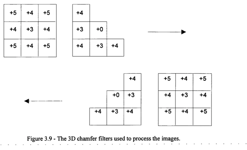
Figure 3.9 - This figure shows the 3D chamfer filters that are used to process the image, and the

direction in which they operate.

Figure 3.10 - Following the first pass of the chamfer filtering process, the image shows distance

values from the object of interest that relate to the direction of this pass only. This then is the

‘intermediate’ image that has resulted from the forward filter pass.

Figure 3.11 - This figure shows the final chamfer filtered image. It is a distance image that has

resulted from running both the forward and reverse filters.

Figure 3.12 - The previous figures showed only schematics of the chamfering method. This

figure shows an example MR image and its resulting chamfer image. The chamfer image,

shown on the right, has its intensities defined by distances away from the object of interest. The

object itself is shown in white for clarity, despite having a distance of zero associated to it.

Figure 4.1 - The formation of the scatterplot. This figure shows how the scatterplot is formed

from two image sets. It is a multidimensional extension of a histogram, with each variable

forming a coordinate axis [39].

Figure 4.2 - On the left of this figure is a single MR slice. This slice has been used in mis­

registration with itself to create a series of scatterplots (shown on the right) that demonstrate

how observations in this feature space (section 4.1.2) disperse as the MR image is mis-aligned

with [a copy of] itself.

Figure 5.1 - This figure shows Vannier’ [idealised] cluster plot [115] (two dimensional) for the

two spin-echo pulse sequences used. It shows the separation of classes achieved in this feature

space, where each ellipse corresponds to a class identified by cluster analysis.

Figure 5.2 - This figure demonstrates how the inappropriate use of cluster seeds can result in

variations in the final segmentations of the scatterplot. As is the case in figure 4.2, we have

used the same image mis-registered with itself to create some dispersion in the feature space.

The image used is shown in the third column of each row. The second column shows the

partitioned scatter plot that results from the misregistration [of the same amount each time], and

from the use of different cluster prototypes. The first column shows the segmentation that

results. The figures are there to illustrate that the clustering procedure’s outcome is often

determined by the cluster seeds chosen.

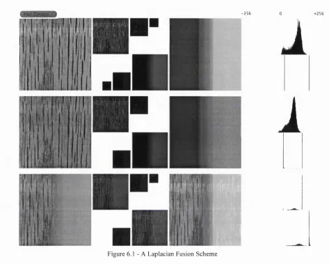
Figure 6.1 - Shown is the concept of ‘local distance’. This shows the Mahalanobis distance

measure being applied across two distributions. It demonstrates the quadratic nature of this

measure, as the distances shown as being equal using the Euclidean measure return different

values when their associated distributions are incorporated into the equation used; i.e., when

using the Mahalanobis distance measure.

Figure 7.1 - This figure demonstrates the inteipolation method used in the project. ‘Nearest

Neighbour Interpolation’ requires that the transformed pixel coordinates are rounded to their

nearest

integer equivalents such that they may then properly act as indices to the image data.

The figure shows just how this woits.

Figure 7.2 - The screen structure of the feature space. This shows how the software written

displayed the feature space on the screen. It basically tells of the transformation used to plot,

with some three-dimensional effect, the image vectors that were used in the segmentation

process.

Figure 7.3 - A crisp partition of the scatterplot using five cluster centres. This figure shows two

windows that were displayed during the execution of the code. In the left window we have four

images. The top two images show a single slice from the two image sets that are to be

registered (in this case the images are MR {on the left), and PET (on the right)). On the

bottom left we have the two input images ‘fused’ with some checkerboard effect. Bottom right

is the segmentation that has resulted from a crisp clustering of the scatterplot, which is shown

in the large window on the right.

Figure 7.4 - This figure has the exact same layout of the above figure, except that the partition

of the scatterplot (right-hand window) has been achieved using a fuzzy clustering algorithm.

The resulting segmentation is shown in the bottom right-hand quarter of the window on the left.

Figure 7.5 - This figure presents a set theoretical representation of the mutual information

measure. This is shown to better explain the equations associated to this section that introduced

Figure 8.1 - This figure shows three images. The left most image is a chamfer filtered version

of the middle image. The two images were then misaligned. The right most image shows the

two images ‘fused’ again using the checkerboard effect. The two images were used as

[artificially complementary] input images to our registration algorithm.

Figure 8.2 - The right-hand half of this figure shows a partitioned scatterplot of two input

images (shown as the top two images in the left-hand side) that has additionally used a medial

feature, and hence we have a three-dimensional feature space. A fusion of the two input images

(corresponding to the same image mis-registered with itself) is shown as a juxtaposed image in

the bottom-left comer. The bottom-right image of the four is the segmentation that resulted

from the partition shown.

Figure 8.3 - This figure shows the segmentation that resulted from a partition of the scatterplot

that did not use the additional medial feature. As before, five cluster prototypes were used.

Figure 8.4 - Dividing this figure into equal thirds, the central third shows a window in which

the four images represent the following (clock-wise fiom top left): an input MR image; an

artificially created nuclear medicine image (created by transforming the intensities of the MR

image), a resulting segmentation of the images; and a colour-oveday [35] fusion of the input

images. The left most third shows the partitioned scatterplot that has resulted from an

alignment

of the two image sets, as well as showing all the input data - in the format of the central most

third - in an insert to its bottom-right comer. The right-hand third shows the partitioned

scatterplot that results from a known misregistration of the two image sets. Its input data is also

shown in its bottom right-hand comer.

Figure 8.5 - Shown are two windows, both containing inserts. The windows display a

partitioned scatterplot that resulted from a known misregistration. The inserts to both of the

images show the input data, their fused image, and their segmentation. The left-hand image has

resulted from a crisp partition of the scatterplot, using five cluster seeds. The right-hand image

has resulted from a fuzzy partition of the scatterplot, which again uses five cluster seeds.

Figure 8.6 - This figure shows two images. The image on the left is a single slice of a CT

volume. The image on the right is a single slice of its associated MR volume. The two image

sets form input to the current registration test.

Figure 8.7 - The image on the right is a partitioned scatterplot (using five cluster centres)

resulting from a misregistration of our MR-CT image pair. TTie image on the left shows the

resulting segmentation.

Figure 8.8 - This figure shows four segmented images. Three of the segmentations, however,

have not resulted from a partition in the scatterplot, but instead from feature spaces derived

from a single image; in this case from the CT image. The first image (far left) shows the

segmentation resulting from the scatterplot alone; and in the maimer previously presented. The

next image results from a segmentation of the CT image using its x-coordiantes, y-coordinates

and pixel intensities as its three features. The third image again uses three features of the CT

image: its z-coordinate value; its intensity values; and a medial measurement. The last image

uses only the CT volume’s medial and intensity values.

Figure 8.9 - This image is a fuzzy segmentation of the CT image that has used just two features:

the CT volume’s medial and intensity values. The better registration results were achieved

using this partition.

Figure 8.10 - The two images shown correspond to the MR (on the left) and PET data sets used

in the final set of tests.

Figure 8.11 - This figure again shows four segmented images. Three segmentations being

derived from the single image; in this case fix)m the MR image (always of an anatomical

image). The first image (far left) shows the segmentation resulting from the scatterplot alone

and in the manner previously presented. The next image results from a segmentation of the MR

image using its x-coordinates, y-coordinates and pixel intensities as its three features. The third

image again uses three features of the MR image: its z-coordinate value; its intensity values;

and a medial measurement. The last image uses only the MR volume’s medial and intensity

values.

Figure 8.12 - This image is a fuzzy segmentation of the MR image that has used just two

features: the MR volume's medial and intensity values.

Appendix Figures

Other (the dynamic image) is

a

the

They are

shown out of registration.

Figure lb (of Appendix II) - This image shows the two objects overlapping. Where the red of

one object overlaps the green of the other, the region is shown in yellow for clarity alone.

Figure 2a (of Appendix II) - Here the two images are shown at a point where the area of overlap

is at its greatest. Here too the measure of mutual information at a maximum.

Figure 2b (of Appendix H) - Here the objects are shown in an intuitive registration. However,

this only corresponds to a point of optima if our similarity measure incorporates an additional

channel [111].

Figure IV. 1 - This figure shows two images that are to be registered. The image on the left is a

single slice of an MR volume. On the right is its corresponding SPET image. This image,

however, has been enhanced about its edges using the ‘Gradient Weighting’ mechanism

described in the thesis.

Figure V.l - Screen structure of the cluster axis. In this section, the eigenvalues and

eigenvectors of each distribution were calculated. To display these [in three-dimensions] on the

screen required the translation that that is described in the text, and shown graphically in this

figure.

Figure

V.n -

This figure shows an example plot of the eigenvectors and eigenvalues about each

of the clusters that have been found using the K-means algorithm.

Figure VII. 1 - This figure demonstrates how a rendering scheme is developed from the raw

image data. Shown are the main points of intersection of a ray cast from the ‘Vantage Point’ in

respect of a light source. The point at which this ray intersects the nearest object to the vantage

point corresponds to the voxel that should be rendered for display.

Jonathan Oakley, Villigen, January 1997

Preface

Often resulting from the simultaneous use of two or more imaging modalities is the need to

compose the single representative form. Only then can the often complementary image

information and the between modality correlations be successfully communicated to an

observer. Of the acquisition processes themselves, neither spatial or temporal performance

characteristics can be assumed as common. Subsequently, research efforts have spawned many

computer-based techniques to perform the methods of image alignment, combination, and

visualisation.

Of the applications, perhaps it is the two researched in this report that best underline the diverse

nature of the field. And although the two pieces of work are thereby related, I shall refer to

them throughout as being the quite independent projects that they were. Their disparity portrays

only a small element of the scope which can be afforded to the subject of ‘Image Fusion.’

The first subject of this work is an investigation into pixel-level fusion methods for combining

Low Light Level intensified images and Thermal images. It is envisaged that these would be

obtained from an airborne platform and used to aid a pilot’s navigation in darkness and other

conditions of poor visibility. The second project is in the field of Medical Imaging, where

different imaging modalities are increasingly called upon to support clinical diagnosis and

surgical planning. Within this discipline, it is the accuracy of the image registration methods

that determines how beneficial a multimodality image fusion scheme can be.

The first project makes perceptual assumptions about the human vision system, which, in the

context of the modalities used, supplies the justification for the fusion process adopted. The

second project uses the characteristics of the imaging modalities to derive the fusion process’s

requisite alignment; an alignment assumed known in the first piece of work. In both cases, it is

only after the images are coregistered that perceptual aspects be exploited in the final

visualisation stage.

The choice to include both of these projects was done so that the report documents my entirety

at UCL. Of the work itself, it is only the second project that claims any originality, as it was on

this that the majority of my time was spent. The first piece of work manages only to

hypothesise about original methods that might have been appropriate (given, of course, quite

forceful arguments), but these were never realised.

The work done toward an automated registration algorithm for medical images contains many

results that my original premises had indicated. Some in-roads have been made towards the goal o f a robust automated registration method. And the use o f such an algorithm supports the means o f viewing the image information in a manner that is significantly clearer and more accurate than conventional methods.

The overall report has turned out to be quite multidisciplinary in flavour, which is nicely characteristic o f the field o f image fusion. Perhaps it is this variety in the studies undertaken that has rendered the tasks o f ‘fusing’ these two pieces o f work into the one composite document difficult. The compromise afforded being to partition the work into two sections, each having its own abstracts, introductions and conclusions.

Abstract - The Optimised Fusion of Low Light Level

(L^) (Intensified) Images and Thermal Images

We begin the first half o f this report with an investigation into a quite specific application o f image fusion. Among the characteristics o f the application were that it used two specific modalities, with some possibility o f their being a third. Also, that it should operate on dynamically changing image sequences, and do so in real-time.

Through the reviewing o f the possible implementation methods to hand, we construct our argument for the use o f one particularly promising method. This favoured a pyramidal image fusion scheme, which, having been implemented, allowed for some closing conclusions to be drawn.

The method o f constructing the pyramidal representation o f individual images was shown to be the key element in determining the effectiveness o f the fusion process. As such, it is this process that therefore commands most o f the project’s attention. Arguments for and against the different kernels that are used to ‘build’ the pyramid come from purely mathematical considerations (e.g., from Baubad [6]), visually enhanced techniques (e.g., Toet [78] and Matsopoulos [52]), and naturally via some computational model that attempts to model the human visual system (Marr et al. [50]). Our aim is to review these and then provide some insight into how a fusion scheme might be implemented given the application.

Abstract - Toward an Automated Medical Image

Registration Algorithm

It is in the field o f Medical Imaging that an increasing number o f relevant imaging modalities have been made available to clinicians. Different modalities often provide complementary information; for example, some are better at showing anatomy, others physiology. As this choice and availability o f image modalities increases, prospects o f image correlation and fusion arise. And as such, it is believed that some combination o f these images will prove requisite to improved clinical diagnosis and treatment.

This project is to do with the combination and the subsequent visualisation o f the different multimodality images. The work involves the registration, or alignment, o f the different image data sets. The registration technique employed attempts to include some notion o f intelligence by incorporating anatomical knowledge and knowledge o f each imager's characteristics.

Work will then require the final visualisation o f the combined image sets, where, ultimately, the success o f any strategy will be dependent on the success o f the registration process.

The layout o f this report reflects this partitioning o f my efforts. The first sections set its context with the literature review. Because o f its importance, this review aims to be comprehensive and I make no excuses for volume; I have put a great deal o f effort into the explanations given, and the knowledgeable reader may skip this. The content focuses on image registration as a prerequisite o f the fusion and visualisation scheme.

We describe our methods in respect o f those in existence, and our results section shows the successes and failings o f each. This is summarised in chapter 9, which details the conclusions o f the work with a realistic look at what has been achieved. It is in the light o f this discussion and the results that we derive a number o f possible applications where our methods might be beneficial. These are developed in my final chapter which ends with a number o f interesting and promising topics o f further work. These no longer remain solely in the bounds o f registration techniques, but are envisaged as natural extensions to the work o f this project such that its importance is substantial and its inclusion relevant.

Contents

Preface... 2

Abstract - The Optimised Fusion o f Low Light Level (L^) (Intensified)

Images and Thermal Images... 4

Abstract - Toward an Automated Medical Image Registration Algorithm.. 5

Contents... 6

1 Introduction - Data Fusion... 16

1.1 M ultisensor F u sio n ...16

1.2 Som e M otivation ... 17

1.3 Exam ple A pproaches... 19

2 Background and Considerations... 20

2.1 Our Operating Environm ent... 20

2.2 Thermal Im a g in g ...21

2.2.1 Sources... 21

2.2.2 Detection... 22

2.3 Passive M illim eter W ave Im a g in g ...23

2.4 Som e P racticalities... 24

2.4.1 Dynamic Range Reduction... 24

2.4.2 Image Restoration...24

2.4.3 Noise Removal... 25

3 Appropriate Levels of Fusion...26

3.1 Where to F u se? ... 27

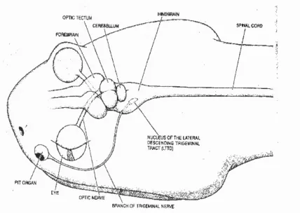
3.1.1 The Infrared ‘Vision’ o f Snakes...27

3.1.2 Optical Mixing - Pointillism ... 28

3.1.3 Cyclopean Vision and Random-Dot Stereograms... 30

4 Toward an Optimal Im age...32

4.1 P hysiological C onsiderations... 33

4 .2 Perceptual C onsiderations... 34

4.2.1 Background... 34

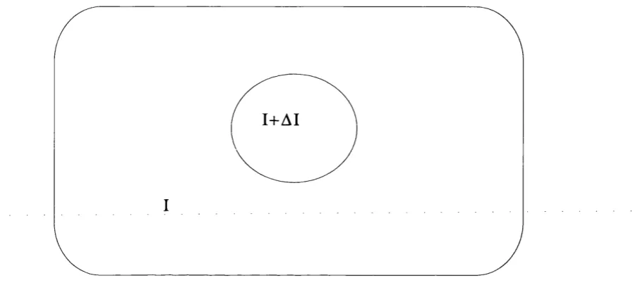
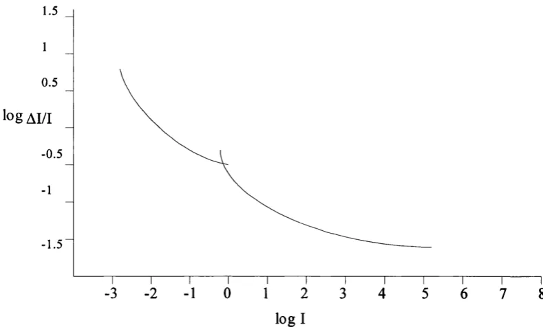
4.2.1.1 The Weber R atio... 34

4.2.1.2 Perceived Brightness...37

4.2.2 Image Quality... 39 4.2.3 Cues for the Focus o f Attention...40 4.2.4 The Role o f Structure... 40

5 Current Image Processing Techniques...43

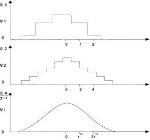
5.1 M ultiresolution A pproaches... 43 5.1.1 Divide-and-Conquer... 44 5.1.2 Pyramidal Representations... 45 5.2 Burt’s Pyram ids...46 5.2.1 The Basic Structure... 46 5.2.2 Producing the Gaussian Pyramid... 48 5.2.2.1 Gaussian Pyramid Interpolation... 50 5.2.2.2 The Laplacian Pyramid... 51 5.3 A pplying the M ultiresolution Approach to Im age F u s io n ... 51 5.3.1 Due to Burt...51 5.3.2 Due to Toet...52 5.4 Choice o f K ernels... 53 5.4.1 The Gaussian-Like Weighting Function... 54 5.4.2 The [Traditional] Gaussian K ernel... 56 5.4.3 Non-Linear Filters...57 5.4.3.1 Mathematical Morphology...58 5.4.3.2 Wavelet Frames... 60 5.4.4 Concluding Remarks... 60 5.5 A Word on Image A lg eb ra ...61 5.6 L ogical Operators...61 5.7 Colour and Pixel O verlay... 62

6 Some Results... 63

6.1 Further C om m ents... 65 6.1.1 Multiresolution Cross-Contrast Optimisation?... 66

7 Future W ork... 68

7.1 Control Structures...68 7.1.1 Bayesian Networks and Rule-Based Systems... 69 7.2 Target R eco g n itio n ... 70 7.3 Hardware Realisation; a Speed and Cost Tradeoff...70 7.4 Im age M anagem ent - Sensor Selection S tra teg ies...71 7.5 Performance E valuation ...71

8 Finally... 72

1 Introduction... 83

1.1 Current Trends...84

2 Characteristics of the Imaging Modalities... 85

2.1 Som e N otion o f Q u a lity ...85 2.2 Traditional (X -R ay) Imaging Techniques; Projection R adiography...86 2.3 X -R ay Transm ission Computed Tomography (C T )...87 2.3.1 CT Image Acquisition... 88 2.3.2 CT’s Image Artifacts... 89 2.3.3 CT’s Role in Planning... 89 2.3.4 Concluding Remarks... 90 2.4 E m ission Computed Tomography (EC T)...90 2.4.1 Positron Emission Tomography (PET)...91 2.4.2 Single Positron Emission Computed Tomography (SPECT)... 93 2.4.3 Quality Control in Emission Computed Tomography... 94 2.5 (Nuclear) M agnetic Resonance Im aging (M R )...96 2.5.1 MR Image Acquisition... 97 2.5.2 MR Image Artifacts... 98 2 .6 Electroencephalography (EEC ) - Electrical Recordings o f the B ra in ... 100 2.7 M agnetoencephalography (M EG) - M agnetic Recordings o f the B r a in ... 101 2.8 Concluding our R eview o f the Imaging M o d a lities... 101

3 Approaches to Image Registration... 103

3.1 A D efinition o f Image R egistration... 104 3.1.1 The Terminology - A Brief word about Points, Markers and Landmarks... 105 3.1.2 Classifying Methods o f Registration... 107 3.2 Som e o f the Underlying M athem atics o f Image R egistration...109 3.3 R eview ing the A pproaches...113 3.3.1 Stereotactic Frame System s... 113 3.3.2 Point Methods using External Markers and Anatomical Landmarks... 113 3.3.3 Curve and Surface Based M ethods... 115 3.3.4 Moment and Principal Axes Methods...121 3.3.5 Correlation M ethods... 123 3.3.6 Interactive Methods...125 3.3.7 Atlas Based Methods... 125 3.4 Exam ple M ethods o f Registration using Anatom ical M arkers... 127 3.4.1 The Head-Hat Algorithm Revisited... 127 3.4.2 The Incorporation o f Priors in Tomographic Reconstruction... 134 3.5 Som e Concluding R em arks... 135

4.1 Background on the Candidate V o x el Based M eth od s...138 4.1.1 Registration o f Multimodality Images using a Region o f Overlap Criterion...138 4.1.2 Woods’ Registration by Minimisation o f Feature Space Dispersion... 141 4.1.3 Grey Value Correlation Techniques used for Automatic Matching o f CT and MR Brain and Spine Im ages...144 4.1.4 Studholme’s Correlation Coefficient... 145 4 .2 The Information Theoretic Approach o f C o U ig n o n ... 146 4.2.1 3D Multimodality Medical Image Registration using Feature Space Clustering.... 147 4.3 Mutual Information as a M easure o f V o x el S im ila rity ... 148 4.3.1 Introducing the Methodology... 149

5 Localising within the Scatterplot the Extent o f the Similarity Measure 153

5.1 A Partition N ecessitated o f the W oods V IR A lg o rith m ... 154 5.2 Outlining H ill’s Original Partitioning E ffort...157 5.3 The Implied N eed for Clustering... 159 5.3.1 The Accurate Segmentation o f MR Images... 160

6 Method... 165

6.1 A n Introduction to Clustering... 165 6.1.2 Clustering Algorithms used in this Project... 166 6.2 Fuzzy Clustering and the Partial V olum e Effect (P V E )... 170 6.2.1 Modelling Uncertainty with Fuzzy Clustering...171 6.2.2 Methods o f Fuzzy Clustering... 172 6.2.2.1 The Fuzzy Membership Function...173 6.3 And Our V o x el Similarity M easures... 174 6.3.1 Defining our Measure o f Mutual Information...174 6.3.2 Defining our Cross-Correlation Measure...175 6.3.3 Defining our Minimum Distance M easure... 175 6.4 Incorporating Additional Channels into a M easure o f Mutual Inform ation...176 6.4.1 Reviewing the Methods... 176 6.5 The N eed for O ptim isation... 179

7 Implementation... 181

7.4 Partitioning the Pattem S p a c e ... 187 7.4.1 Vector Assignment... 187 7.4.2 The Use o f the Medial Feature... 188 7.5 Im age Segm en tation ... 190 7.6 C lassification S c h e m e ... 191 7.7 Clustering Procedures...191 7.7.1 Distance Computation... 193 7.7.2 Cluster Membership...193 7.8 The U se o f Cluster A ffinities in the Registration P rocess...196 7.9 Im plem enting the Additional Channels... 197 7.9.1 Our Intended Use o f the Extra Channels...198 7 .1 0 The O ptim isation Process U sed in this P ro ject...199 7.11.1 Brent’s Method in One-Dimension... 200 7.10.2 Direction Set (Powell’s) Methods in M ultidimensions...201 7.10.2.1 The Use o f Derivatives in the Parameter Search...201

8 Registration Results... 204

8.1 The Worth o f the Entropy M easure... 205 8.2 Benchm arking the R esu lts...207 8.3 Initial testing o f a Segm entation Step... 208 8.3.1 A Test o f Feasibility... 208 8.3.2 D iscussion...210 8.3.3 In Terms o f Efficiency... 212 8.4 The Worth o f the M edial Feature?... 213 8.5 A Rather Synthetic M ultimodal T est...214 8.6 A First M ultimodal Test - Patient 0 ... 216 8.6.1 Tracing out the Measure o f Mutual Information... 219 8.7 Patient 1 ... 222 8.7.1 Further Tracing o f the Mutual Information Measure - Patient 1 ... 222 8.7.2 Registration Results - Patient 1...224 8.8 R efining the Segm entations U sed - Patient 1 ... 225 8.8.1 Interpreting the Results...227 8.9 Tests for Patient 2 ... 229 8.9.1 Registration Results - Patient 2 ...230

9 Conclusions o f the Registration Work...233

9.1 Summary o f the W ork... 233 9.2 V alidating the Various Efforts... 234 9.3 Sum m arising the R esu lts... 234 9.4.1 The Worth o f Different Segmentation Methods... 235

9.4.1.1 A Crisp Segmentation o f the Scatterplot...235 9.4.1.2 The Effect o f the Medial Feature...235 9.4.1.3 A Fuzzy Segmentation o f the Scatterplot... 236 9.4.2 Other Segmentations; Efforts Resembling Established Methods?...238 9 .5 The U se o f Additional C h annels...238 9.5.1 With Gradient Weighting...239 9 .6 L im itations... 2 40 9 .7 Future Work - Registration B a se d ... 241 9 .8 F inally...241

10 Future Work... 244

10.1 Further Work on our Registration M e th o d s... 244 10.1.1 In Respect o f the Segmentation... 244 10.2 Interpretation o f Functional Im ages w ith the aid o f A natom ical Im a g e s ... 245 10.2.1 The Further Intentions for the Scatterplot as our Information Processing Environment... 247 10.2.2 Anatomical Localisation for PET using MR...250 10.3 Com bining the M ethods - A n A ll-Singing, A ll-D ancing S chem e?... 254 10.4 C losing remarks... 255

11 References... 257

Appendix II - Toward an Understanding o f the Measure o f Mutual

Information’s Behaviour... 274

II. 1 V io la ’s Aligrunent by M axim ization o f Mutual Inform ation... 274 II. 1.1 Description o f Method...275 II. 1.2 Stochastic Maximization o f Mutual Information... 276 II. 1.3 MR Alignment due to V iola... 277 II.2 A Preliminary Study and History o f the M easure... 278 11.2.1 [An] Introduction [to Entropy]...278 11.2.2 What is there to learn?...279 11.2.3 So what is the Formal Definition o f these Entropy Measures?...279 11.2.4 So how are we going to Investigate these?...279 11.2.5 So what happened?... 281 11.2.6 Discussion - What N ext?...282 11.2.7 Using Additional Channels... 282

Appendix III Traces for the Multimodal Test about Various Clusters

-Patient 0 ...284

Appendix IV - Gradient Weighting (GW )... 286

IV .2 U sing the First Derivatives o f the Image D a ta ... 286 IV .3 M ethod - the Sobel Operator...287 IV .4 Variations due to Gradient W e ig h tin g ...288 IV .5 Variations across C lusters... 289 IV .6 Traces described in this A p p e n d ix ...291 IV.6.1 Results o f traces for shifts about the Y-axis and rotations about the Z -axis...291 IV.6.2 Results o f traces for shifts about the X-axis and rotations about the Z -axis...291 IV.6.3 Results o f traces for shifts about the X- and Y -a x es... 292

Appendix V - Using the Eigenvalues and Eigenvectors...293

V .l Som e C o n tex t... 293 V .2 Calculation o f the E igenvalues and E ig en v ecto rs... 294 V .3 Its U s e ... 295

Appendix VI Multimodality Image Fusion and Visualisation... 296

VII. 1 Som e Exam ple A pplications... 297 VII.2 D isplay and V isu a lisa tio n ... 298 VII.2.1 Accessing the Information... 299 VII.2.2 Rendering...300 VII.2.3 Multiresolution Image Fusion... 304 VII.2.4 Colour and Pixel Overlay... 304 VII.2.5 Colour Encoding...306

Project 1:

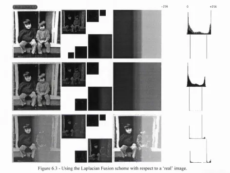
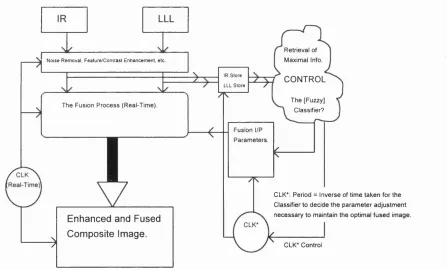
Figure 2.1 - Electromagnetic Spectrum...22 Figure 3.1 - The physiology o f the brain and nerve pathways o f the snake... 28 Figure 3.2 - Suerat’s Optical Pointillism...29 Figure 3.3 - A Random-dot Auto-Stereogram... 30 Figure 4.1 - The basic setup used to characterise brightness discrimination... 35 Figure 4.2 - Typical Weber ratio as a function o f intensity...36 Figure 4.3 - Mach Bands... 38 Figure 4.4 - Simultaneous Contrast...39 Figure 5.1 - The Engineering Approximation to the Laplacian... 48 Figure 5.2 - A graphical representation o f local averaging...49 Figure 5.3 - The first 4 levels o f the Gaussian Pyramid...50 Figure 5.4 - The first 4 levels o f the Gaussian and Laplacian Pyramid... 51 Figure 5.5 - The Equivalent Weighting Funtion...55 Figure 6.1 - A Laplacian Fusion Scheme...64 Figure 6.2 - The results o f ORing the two input images... 65 Figure 6.3 - Using the Laplacian Fusion scheme with respect to a ‘real’ image... 66 Figure 7.1 - Block Diagram o f an Example Control System for our Fusion Scheme...69

Project 2:

Figure 3.3 - The centroid from which rays intersect surfaces...117 Figure 3.4 - An intuitive alignment o f the image sets... 118 Figure 3.5 - The basic algorithm; points o f obvious disagreement upset the process... 118 Figure 3.6 The principal axes o f an ellipsoidal object... 122 Figure 3.7 - The original thresholded image... 130 Figure 3.8 - The image ‘prepared’ for chamfering...130 Figure 3.9 - The 3D chamfer filters used to process the images... 131 Figure 3.10 - The ‘intermediate’ image (resulting from running the forward filter pass) 131 Figure 3.11 - The final image...131 Figure 3.12 - A typical MR image and its resulting chamfer image...133 Figure 4.1 - The Formation o f the Scatterplot... 142 Figure 4.2 - An MR image from which the feature space diagrams were derived... 144 Figure 5.1 - Vannier’s [Idealised] Scatterplot... 162 Figure 5.2 - Variation in partitions due to variation in the initial cluster prototypes... 164 Figure 6.1 - The Mahalanobis Distance Measure...169 Figure 7.1 - Nearest Neighbour Interpolation... 186 Figure 7.2 - The Screen Structure o f the Feature Space...190 Figure 7.3 - A Crisp Partition o f the Scatterplot using five clusters...195 Figure 7.5 - A Fuzzy Partition o f the Scatterplot using five clusters...195 Figure 7.6 - The Set Theoretical Representation o f the Measure o f Mutual Information 198 Figure 8.1 - Verifying the Entropy Measure on a Chamfered Image... 205 Figure 8.2 - The segmentation on which the initial registration tests were run...210 Figure 8.3 - The segmentation o f the image set without using the medial feature... 213 Figure 8.4 - A Synthetic Multimodal Test... 215 Figure 8.5 - The Registration problem - Patient 0 ... 217 Figure 8.6 - The different Modality Image Sets from Patient 1 (CT and MR)...222 Figure 8.7 - The Nature o f the Segmented Image Sets for Patient 1... 225 Figure 8.8 - Different Segmentations for Patient 1 Images...228 Figure 8.9 - The fuzzy segmentation o f test 4 ...229 Figure 8.10 - The MR and PET images o f Patient 2 ...230 Figure 8.11 - Different Segmentations for Patient 1 Images...230 Figure 8.12 - The fuzzy segmentation o f test 4 ...232 Figure IV. 1 - The Effective Edge Enhanced Image due to GW... 289 Figure V .l - Screen structure o f the cluster axis...294 Figure V.2 - How the Eigensytem is actually shown...295 Figure VI. 1 - The rendering o f an image...302

Acknowledgments

Project One: The Optimised Fusion of Low Light

Level (L^) (Intensified) Images and Thermal

Images

1 Introduction - Data Fusion

There is no broadly accepted definition o f data fusion. It is a field that has generated a significant amount o f interest among researchers from a variety o f engineering disciplines, directly or otherwise. In imaging, its approaches combine information made available from different sources, thus generally enabling a better understanding o f a given scene or environment. As such, it poses the problem o f constructing a single model o f some environment from variously sourced data.

The motivation for using multiple sensors in a system can be considered as the response to the question: if a single sensor can increase the capability o f a system, would the use o f more sensors increase it even further [1]? In one sense, the value o f the combined information that the sensors provide is hoped to be greater than the sum o f the value o f the information provided separately; the effect o f synergy.

Our problem area falls into the domain o f data fusion. As a subset o f such a vast topic, this paper can only outline some o f its purpose and methods, whittling the subject area down via sensor fusion to then concentrate on image fusion alone.

1.1 Multisensor Fusion

At a practical level, sensor fusion is the technology that allows us to collect data through multiple sensors, thereby enabling us to increase our knowledge, accuracy and the confidence with which we may apply this. In general, we must model and prioritise the sources to make best use o f the information and the most sense o f the particular environment. This is a constraint satisfaction problem that distinguishes some intelligent sensor [or indeed, image] fusion system from simple additive integration systems. But what exactly are our constraints? And what exactly are we trying to model?