Oil Prices, Exchange Rates,
And Inflation Expectations In South Africa
Kin Sibanda, Ph.D. Student, University of Fort Hare, South AfricaProgress Hove, Ph.D. Student, Vaal University of Technology, South Africa Genius Murwirapachena, Durban University of Technology, South Africa
ABSTRACT
Informed inflation expectations facilitate the extemporisation of a proper monetary policy framework that allows for the achievement of economic objectives, among them price stability. This study used the vector autoregression model to assess the impact of crude oil prices and exchange rates on inflation expectations in South Africa. Monthly time-series data for the period July 2002 to March 2013, obtained from the electronic database of the South African Reserve Bank were used. The study obtained statistically significant results suggesting that both crude oil prices and the exchange rates have a positive impact on inflation expectations in South Africa. Keywords: South Africa; Oil Price; Inflation Expectation; Exchange Rate; Vector Autoregression Model
INTRODUCTION
ver the past three decades, most governments have been realizing the increasing importance of inflation expectations through their self-fulfilling effect on actual inflation, and hyperinflation where the expectations are left uncontrolled (Ueda, 2011). Previous studies revealed that well anchored inflation expectations enable the monetary authorities to achieve other monetary policy objectives such as economic growth and price stability (Mboweni, 2003 and Ueda, 2011). Given the importance of inflation expectations in influencing the monetary policies of nations, governments in both developed countries (for example New Zealand in 1990) and developing countries (for example South Africa in 2000) adopted the inflation targeting monetary policy framework. According to Mboweni, (2003), inflation targeting provides an anchor for inflation expectations and price as well as wage setting, ultimately reducing the friction that arises from widely divergent inflation expectations. A plethora of recent empirical literature supports the implementation of inflation targeting as a monetary policy tool that anchors inflation expectations by households, (Mohanty, 2012), inflation forecasting (Bernanke, 2007) as well as the public attitudes to inflation and interest rates (Driver and Windram , 2007).
The success of a nation’s monetary policy framework depends on how the inflation expectations were formed, that is, it is imperative to consider the antecedents of inflation expectations in a country, as they play a major role in the formation of inflation expectations. Previous literature has investigated the factors affecting realized inflation (Niyimbanira, 2013; Celik and Akgul, 2011) and less has been done on the factors affecting inflation expectations. For those studies that sought to explore the determinants of inflation expectations, the main focus was on developed nations such as Turkey (Celik and Akgul, 2011), United States of America (Curtin, 2009 and Ueda, 2010) as well as Japan (Ueda, 2010) and rarely can one find such studies in the South African context. Empirical studies revealed the common determinants of inflation expectations to be changes in energy and food prices, oil price shocks, interest rates and exchange rates (see Nkomo, 2006 and Wakeford, 2006).
prices and inflation expectations as well as the relationship between real exchange rates and inflation expectations in South Africa. Specifically, this paper seeks to assess the impact of both oil prices and exchange rates on inflation targeting in South Africa.
This paper consists of six sections. The section subsequent to this gives an overview of trends in the explored variables while the third section gives a bried review of empirical literature. The fourth section gives the methodology used in the study while the fifth section presents empirical tests and results. Finally, an interpretation of results and a conclusion are presented in the sixth.
An overview of South Africa’s inflation expectations, oil prices and exchange rates
South Africa endured variations in the inflation expectations, oil prices and exchange rates from 2002 till present. Both oil prices and nominal exchange rates are volatile and their movements have significant impact on household inflation expectations. In 2000, South Africa adopted the inflation targeting policy which puts price stability as the primary objective of monetary policy. Monetary policy works in part by influencing inflation expectations which makes inflation targeting important. Mboweni (2003) argued that inflation targeting sets a clear inflation objective and a commitment to achieve. In so doing, the central bank is able to anchor the household inflation expectations, thus improving planning for the economy, as well as providing an anchor for expectations of future inflation to influence price and wage setting. Trends in South African expected inflation for the period 2002 to 2013 are shown in Figure 1.
Figure 1. Expected inflation trends 2002-2012
Source: Author’s own graph with data from the SARB (2014)
Figure 1 shows that inflation expectations responded positively to the inflation targeting policy over the years. The year 2002 the inflation expectations were high and the official inflation target could not be reached. This was the case because the terrorist attack in the US on September 11, combined with massive depreciation of South African Rand put high pressure on CPIX inflation, which reached high levels in 2002 (Saunders, 2004). The increase in inflation in 2002 prompted the Reserve Bank to react by increasing the repo rate. Hence, from 2003 to around 2006, inflation expectations were declining from 9.4 per cent in the fourth quarter of 2002 to 4.4 per cent in the second quarter of 2006. The decrease in inflation expectations during this period can be attributed to the appreciation of the Rand and lower food prices. The expectations for most parts between 2002 third quarter and 2007 were within the target range of between 3-6 percent and 3-5 percent for the year 2004 expect for the year 2002 and 2003 were the expectations were above 7.3 percent culminating from the depreciation of the exchange rate in 2001. From the third quarter of 2006 the inflation expectations gradually started picking up until the fourth quarter of 2008 were it reached the highest of 10.7 percent as depicted by figure 1. This increase is attributable to external factors such as the 2008 world food price crises, the rise in oil prices and the global financial crisis of 2007-2009. From the year 2010 the inflation expectations took a gradual downward trend but outside the set target. People
anticipated a decline in inflation but not enough to reach the 3-6 per cent target; except for the year 2011 were it averaged 5.3 percent. Marcus (2013) attributed this deterioration in the inflation outlook to the exchange rate depreciation. A comparison of trends in the expected inflation and crude oil prices for the period 2002 to 2013 is shown in Figure 2.
Figure 2. Expected inflation and crude oil price trends 2002-2012
Source: Author’s own graph with data from the SARB (2014)
Figure 2 depicts the pictorial relationship between crude oil prices and expected inflation. The graph shows that generally the two graphs follow each other save for the period between 2002 and 2004. Crude oil prices have been gradually increasing since 2002 until the second quarter of 2008 second quarter were it reached US$121.31 per barrel. During this period inflation expectations were on the increase (except for 2002-2004). Crude oil prices then dropped to US$44.49 a barrel in 2009 first quarter. This was followed by downward trend in inflation expectations as depicted by Figure 2. From the second quarter of 2009 the crude oil prices have been gradually increasing followed by gradual but stable increase in the inflation expectations. The positive correlation between the two variables is due to the fact that oil is important in South Africa both as an input and energy, therefore, an increase in oil prices leads to people expecting an increase in actual inflation. To gain more insight on expected inflation in South Africa, Figure 3 gives a comparison of its trends and the nominal exchange rate for the period 2002 to 2013. The comparison of these two phenomena is because fluctuations in the exchange rate are an important antecedent of inflation expectations. 0 20 40 60 80 100 120 140 0 2 4 6 8 10 12 2002Q 3 2003Q 2 2004Q 1 2004Q 4 2005Q 3 2006Q 2 2007Q 1 2007Q 4 2008Q 3 2009Q 2 2010Q 1 2010Q 4 201 1Q 3 2012Q 2 C ru d e O il P ri ce s (U S $/ b ar re l) Exp ec te d I n fl ati on r ate Years
Figure 3. Expected inflation and nominal exchange rate trends 2002-2012
Source: Author’s own graph with data from the SARB (2014)
Figure 3 shows a negative relationship between nominal exchange rate and inflation expectations. When the currency depreciates people anticipate that inflation will increase in the near future. As shown in Figure 3, the rapid rand’s rapid depreciation in late 2001 led to greater inflationary pressure which led to a rise in the expected inflation especially for the years 2002 and 2003 where inflation expectations averaged 8.4 per cent. From the year 2004 to 2007, the graph depicts decreasing nominal effective exchange rates appreciated coupled with low and declining inflation expectations. The first quarter of 2006 had a stronger nominal effective exchange rate of 95.81 corresponding to the lowest inflation expectation of 4.4 per cent. Between the period 2008 and 2009 the rand exchange rate depreciated while at the same time the expected inflation was very high. After 2010 the rand gradually peaked and during this time the inflation expectations dropped. However, the last quarter of 2011 and first quarter of 2012 encountered depreciation in the nominal effective exchange rate from 72.9 in 2011 third quarter to 65.59 in 2012 first quarter and during this period inflation expectations started to increase. Possible causes of this increase are increasing oil prices, depreciating exchange rate and food prices (Marcus, 2013). Generally, Figure 3 shows a positive relationship between exchange rates and inflation expectations.
LITERATURE REVIEW
The paper uses the variant of adaptive behaviour as well as the rational expectations as the theoretical foundations for inflation expectations. On one hand, the variant of adaptive behaviour is premised on the assumption that expectations are formed through the estimation and inference of the known past and current experience into the unknown future. People also use new commonly available information to speculate and make inferences into the future. For instance, if oil prices increase, people may use their past and current known experience together with the common knowledge on what happens when oil prices increase and may expect the overall inflation to rise. Nevertheless, people’s inflation expectations may not change continuously, as such, they may peg their revisions regularly. According to Mohanty (2012), the key feature of these changes of inflation expectation is that it is largely backward-looking. On the other hand, the rational expectations theory holds that if the economic agents form their inflation expectations after considering all the available and known information together with the reaction function of the monetary authority, their inflation expectation could be considered as rational (Mohanty, 2012). Economists in practice, derive the inflation expectations value from the complex rational expectations models (Mohanty, 2012). The next section provides an empirical literature review.
0 20 40 60 80 100 120 0 2 4 6 8 10 12 2002Q 3 2003Q 2 2004Q 1 2004Q 4 2005Q 3 2006Q 2 2007Q 1 2007Q 4 2008Q 3 2009Q 2 2010Q 1 2010Q 4 201 1Q 3 2012Q 2 N omi n al Exc h an ge R ate Exp ec te d I n fl ati om R ate Year
Empirical Literature Review
A plethora of empirical literature exists on the impact of both oil prices and exchange rates on inflation expectations. Most of these were done on developed countries and include the works of Ueda (2010) as well as Segal (2011) Studies have also been conducted in emerging economies such as Turkey (see Celik and Akgul, 2011) In the South African context, available literature does not examine a combination of the variables explored in this study (Nkomo, 2006; Chisadza, et al., 2013 as well as Niyimbanira, 2013). This section provides a review of literature related to the relationship between oil prices, exchange rates and inflation expectations. The section includes literature both South Africa and other countries (developed and less developed).
Ueda (2010) employed the Vector Auto-Regression (VAR) model to examine the determinants of inflation expectations in Japan and the United States of America. The study used survey data on households’ inflation expectations for Japan and the US, and found that inflation expectations adjust more quickly than actual inflation to the changes in exogenous prices and to monetary policy shocks. It was also revealed in the study that when compared with Japan, the effects of the exogenous prices on inflation and inflation expectations were large and long termed in the United States of America, and also that the shocks to expectations had self-fulfilling effects on inflation.
Segal (2011) followed a literature analysis methodology to investigate the impact of oil price shocks on the macro economy. The paper sought to explain why the rise in oil prices up to 2008 had little impact on the world economy. The study revealed that high oil prices have never been as important as they are popularly thought to be. In addition, the findings of this study showed that high oil prices have not reduced growth in recent years because they no longer pass through to the core inflation. As a result there was no evidence of monetary tightening previously seen in response to high oil prices. The study also revealed that oil prices had little impact on the global recession of 2008-2009.
Celik and Akgul (2011) examined the relationship between the consumer price index (CPI) and the fuel oil price index in Turkey, using the Vector Error Correction Model (VECM). The study used the time interval monthly data of the period 2005-2010. The findings of the study revealed that a 1% increase in fuel oil prices caused the CPI to rise by 1.26% with an approximate one year lag. More so, the changes in fuel oil prices were found to be the one way Granger cause for changes in the CPI.
In South Africa, Chisadza, et al. (2013) investigated the impact of oil supply and demand shocks on the South African economy, using a sign restriction-based structural Vector Auto-Regressive (VAR) model. Their findings revealed that an oil supply shock has a short-lived significant impact only on the inflation rate, while the impact on other variables was statistically insignificant. More so, their study reported a negative reaction to oil specific demand shocks of inflation rate and real exchange rate. The study also revealed that unanticipated changes in oil prices resulting from speculations have a positive impact on output.
Nkomo (2006) conducted a study on crude oil price movements and their impact on South Africa. Using a history and literature analysis method, the study concluded that South Africa has been shielded from much of the negative impacts of crude oil price increases because of its strong US Dollar/Rand exchange rate, though vulnerable to external sources of oil supply and to increases in international oil prices. The study also concluded that the immediate impact of high crude oil prices is on economic growth and development of the oil consuming country.
Niyimbanira (2013) used the Johansen-Juselius co-integration method to investigate the relationship between oil price and inflation in South Africa. The study employed to test the long run relationship between oil prices and inflation. Results from the study revealed a co-integration relationship between oil prices and inflation in South Africa. In addition, a unidirectional causality running form the oil prices to inflation was also revealed.
decreased the exchange rate pass-through into import, producer and consumer prices. The next section assesses the trends in inflation expectations, oil prices and nominal exchange rates.
The empirical literature reviewed revealed that oil prices and exchange rates have a significant impact on inflation expectations across the world. The other possible drivers on the inflation expectations common in previous studies are interest rates and food prices. The next section presents the model, results and analysis.
DATA AND METHODOLOGY
This study employs monthly time series data covering the period July 2002 to March 2013. Data for all the variables were obtained from the electronic database of the South African Reserve Bank (SARB).
Empirical Model Specification
To examine the impact of oil prices and exchange rates on inflation expectations in South Africa, this study uses the cointegration method as used by Niyimbanira (2013) who investigated the relationship between oil prices and inflation in South Africa. The study modified Niyimbanira’s model to examine the impact of oil prices and exchange rates on inflation expectations. Other relevant explanatory variables are also included and the model used will be of the form:
EXPECT
t=
β0
+
β1
OIL
t+
β2
EXCH
t+
β3
INTREST
t+
β4
FOOD
t+ e
t 1.1where:
EXPECT: Inflation expectations can be broadly defined as economic agents’ belief or views or perceptions about inflation in the future. Inflation expectations are expressed as a percentage.
OIL: Crude oil prices in US$ per barrel (nominal/real values).
EXCH: Exchange rate. This is nominal exchange rate of South Africa rand per US dollar foreign exchange rate.
INTR: Exchange rate. This is nominal exchange rate of South Africa rand per US dollar foreign exchange rate.
FOOD: Final consumption expenditure by households on food, beverages and tobacco.
Β0 – β4: Coefficients et: Error term t: Time variant Estimation Techniques
The econometric model used to estimate the impact of oil prices and exchange rates on inflation expectations in this study proceeds in two steps. Firstly, the co-integration of inflation expectations, oil prices and exchange rates are examined by testing for stationarity in these series. If the series are integrated of the same order, it suggests that a co-integrating vector can be found and the variable is stationary. Secondly, the co-integration residual is used as an error correction term leading to the estimation of both the short run effects and the speed of adjustment. Subsequent to the two steps are diagnostic checks which will be performed to test for heteroskedasticity, autocorrelation and normality. Impulse response analysis and variance decomposition will also be performed.
implies that the usual t-ratios will not follow a t-distribution and the F-statistic will not follow an F-distribution. Therefore, unit root tests should be done on all the series used before estimating the parameters and testing for co-integration so as to avoid spurious and or nonsense regression. The adopted ADF is given by the equation:
Δyt=µ+λt+(γ−1 )yt−1
t=1 p
∑ γjΔyt−1+et (1.2)
The ADF (Dickey and Fuller, 1981) equation given in 1.2 allows for an AR process that may include a non-zero overall mean for the series and trend variable . The special case where corresponds to the Dickey-Fuller (DF) test. The test statistic of the Augmented Dickey-Fuller would be invalidated if the residual of the reduced form equation were auto-correlated. In order to test the null hypothesis of non-stationarity, the t-statistic of the estimate of is compared with the corresponding critical values, calculated by Dickey and Fuller. The number of lags of y to include in equation 1.2 and whether to include a constant as well as a trend variable are important factors to consider. To make this choice the adjusted R2 and the
Schwartz (1978) Criterion is used.
The Phillips-Perron (PP) test is a more robust unit root test that may be applied together with a DF-style test. This is because DF-style tests are commonly criticised for having low power (Gujarati, 2003), and tend to accept the null hypothesis of unit root more frequently than is warranted (Baum, 2001). The test regression for the PP test is given as:
y
t=
β0+ py
t-1+ e
t (1.3)The PP test corrects for high order serial correlation by adding lagged differenced terms on the right-hand side. It makes a correction to the t-statistic of the coefficient from the regression to account for the serial correlation in the error term. The PP test statistics can be viewed as DF statistics that have been made robust to serial correlation by using the Newey-West (1987) heteroskedasticity- and autocorrelation-consistent covariance matrix estimator.
After establishing the order of integration, the study proceeds to determine the existence of a long-term relationship between the investigated variables. To perform this, the study uses the Johansen cointegration technique which produces two statistics, these are, the likelihood ratio test based on maximal eigenvalue of the stochastic matrix and the test based on trace of the stochastic matrix. These two statistics are then used to determine the number of cointegrating vectors. The test is based around an examination of the π matrix which can be interpreted as a long-run coefficient matrix. The test for cointegration between the variables is calculated by looking at the rank of the π matrix via its eigenvalues. The value π is defined as a product of two matrices:
π
=
α
β
’
(1.4)The matrix β gives the cointegrating vectors, while α gives the amount of each cointegrating vector
entering each equation of the vector error correction model which is also called the adjustment parameter. Under the maximum eigenvalue ( test, the null hypothesis that rank (Π) = is tested against the hypothesis that the rank is +1. The null hypothesis demonstrates that there is cointegrating vectors and that there are up to cointegrating relationships, while the alternative suggests that there is ( +1) vectors.
The test statistics are based on the eigen-values obtained from the estimation procedure. This involves ordering the largest eigenvalues in descending order and considering whether they are significantly different zero. The rank of Π is zero if the variables are not cointegrated, thus all the characteristic roots will be equal to zero. To test for the numbers of the eigen-values that are significantly different from zero, the following statistic is used in the maximum eigenvalue:
)
(
p
)
(
t
p
=
1
t t
t
t
y
e
y
=
+
+
−
+
Δ
µ
λ
(
γ
1
)
−1)
1
(
γ
−
ρ
)
max
λ
r
r
r
λ
max( r,r
+
1 )
=
−
TIn( 1
−
λ
ˆ
r+1)
(1.5) The second method is the trace statistic, which is based on a likelihood ratio test about the trace of the matrix. This statistic considers whether the trace is increased by adding more eigenvalues beyond the rth eigenvalue.The number of cointegrating vectors in this case will be less than or equal to . Just like under the maximum eigenvalue, in the event that , the trace statistic will be equal to zero as well. Separately, the closer the eigenvalue are to a unit the more negative is the ln (1- term and therefore, the larger the trace statistic. In this case, the trace statistic is calculated by:
Determining the presence of cointegration is a procedure which involves working downwards and stopping at the value of associated with a test statistic that exceeds the displayed critical value. The Eviews econometrics software provides critical values for both the maximum eigenvalue and trace statistic.
After the number of cointegrating vectors is established, the study proceeds with the estimation of the vector error correction model (VECM). This applies the maximum likelihood estimation of VAR to simultaneously determine the long-run and short-run determinants of the expected inflation. The approach considers the short-term adjustments of the variables as well as the speed of adjustment of the coefficients. The VECM specification is of the form:
Δ t =
where is the 7×1 vector, are all integrated of order 0, is a7×7 coefficient matrix and
is an error term normally and independently distributed.
Once the short and long run impact of oil prices and the exchange rates on expected inflation are established, the study proceeds to perform diagnostic checks. These checks are crucial because they validate the parameter estimation outcomes achieved by the estimated model. Diagnostic checks performed in this study test for the stochastic properties of the model such as heteroskedasticity (White test), autocorrelation (Lagrange Multiplier) and normality (Jarque-Bera). The study also tests for stability in the model using the Ramsey RESET and the CUSUM tests. To trace the responsiveness of expected inflation to shocks in oil prices as well as the exchange rate; and to measure the proportion of forecast error variance in expected inflation that is explained by innovations in itself and the other variables, this study will respectively perform an impulse response analysis and variance decomposition.
EMPIRICAL RESULTS
The first commission in our econometric analysis was to test for stationarity (unit root) in the time series properties of our data. Unit root tests were performed using the Augmented Dickey-Fuller (ADF) and the Phillips-Peron (PP) tests. Results obtained from the tests in levels and when the data were first differenced are respectively given in Tables 1 and 2.
r
0 ^
= i
λ
)
^
i
λ
) 6 . 1 ( )
1 ln( )
(
1
^ 1
∑
+ =+
− −
= n
r i
r
trace r T
λ
λ
r
y
1∑
1(
1
.
7
)
= −
−
+
Γ
Δ
+
Π
y
t tki iy
tε
kt....)
(
1 2t ty
y
y
=
+
Δ
y
tΓ
ikt
Table 1. Unit Root Tests - Level Series
Augmented Dickey Fuller Phillips Peron
Variable Intercept Trend and Intercept Intercept Trend and Intercept
EXPECT -2.780148* -2.727430 -1.789709 -1.744690
OIL -1.911687 -3.481624** -1.646156 -3.046642
EXCH -3.275199** -3.787046** -2.519147 -2.754881
INTREST -2.924710** -3.068915 -1.589165 -1.843330
FOOD 1.198091 -1.461709 1.134860 -1.184189
Notes: *, **, *** indicates significance at 10%, 5% and 1%
Table 2. Unit Root Tests - First Differences
Augmented Dickey Fuller Phillips Peron
Variable Intercept Trend and Intercept Intercept Trend and Intercept
ΔEXPECT -4.779775*** -4.867065*** -11.39224*** -11.36315***
ΔOIL -7.449115*** -7.420011*** -7.467835*** -7.438773***
ΔEXCH -7.552487*** -7.911857*** -7.643658*** -7.841650***
ΔINTEREST -3.556676*** -3.599672** -10.40452*** -10.37293***
ΔFOOD -3.563717*** -3.845271** -6.441665*** -6.710123***
Notes: *, **, *** indicates significance at 10%, 5% and 1%
As shown in Tables 1 and 2, unit root test results from both ADF and PP indicate that the variables are mostly not stationery in level series and are all stationary when first differenced. Since the series are stationary after being first differenced, this means that the variables are integrated of the first order, I(1), thereby satisfying the requirement for the Johansen and Juselius (1990) cointegration test which can only be adopted if the observed variables are I(1).
The other precondition for the Johansen and Juselius (1990) cointegration test is to determine the lag length which is econometrically determined using different information criterions. In this study, one lag in differences (two lags in levels) is used when testing for cointegration. Results from the Johansen and Juselius cointegration test are shown in Table 3.
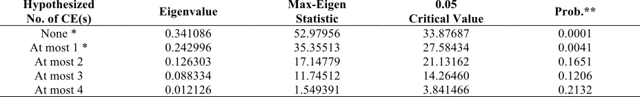
Table 3. Cointegration Test Results
Date: 05/04/14 Time: 13:07. Sample (adjusted): 2002M09 2013M03. Included observations: 127 after adjustments. Trend assumption: Linear deterministic trend. Series: EXPECT OIL EXCH INTREST FOOD. Lags interval (in first differences): 1 to 1.
Unrestricted Cointegration Rank Test (Trace) Hypothesized
No. of CE(s) Eigenvalue
Trace Statistic
0.05
Critical Value Prob.**
None * 0.341086 118.7770 69.81889 0.0000
At most 1 * 0.242996 65.79742 47.85613 0.0005
At most 2 * 0.126303 30.44229 29.79707 0.0421
At most 3 0.088334 13.29451 15.49471 0.1044
At most 4 0.012126 1.549391 3.841466 0.2132
Trace test indicates 3 cointegrating eqn(s) at the 0.05 level * denotes rejection of the hypothesis at the 0.05 level **MacKinnon-Haug-Michelis (1999) p-values
Unrestricted Cointegration Rank Test (Maximum Eigenvalue) Hypothesized
No. of CE(s) Eigenvalue Max-Eigen Statistic Critical Value 0.05 Prob.**
None * 0.341086 52.97956 33.87687 0.0001
At most 1 * 0.242996 35.35513 27.58434 0.0041
At most 2 0.126303 17.14779 21.13162 0.1651
At most 3 0.088334 11.74512 14.26460 0.1206
At most 4 0.012126 1.549391 3.841466 0.2132
The results indicate that at least three cointegrating equations exist at 5 per cent significance level using the trace test while at least two equations are reflected to exist in the maximum eigenvalue test. This implies that there is a long run relationship between expected inflation and its selected determinants. The null hypothesis of no cointegrating vectors is rejected since the trace statistics and the max-eigen statistics of the indicated number of cointegrating equations in both the rank and max-eigen tests are greater than the critical values at 5 per cent significance level.
Subsequent to establishing the presence of cointegration, this study examined the short-term behaviour of the variables. The study uses the Vector Error Correction Model (VECM) to disaggregate the short run and long run effects of crude oil prices (OIL), exchange rates (EXCH), interest rates (INTREST) and the cost of food (FOOD) on inflation expectations (EXPECT) in South Africa. VECM results showing the long run relationships between EXPECT and its selected determinants are presented in Table 4.
Table 4. Long-run Cointegration Equation of EXPECT
OIL EXCH INTREST FOOD C
Coefficient 0.618356 9.948344 -2.507330 -1.414141 2.771722
Standard Errors (0.07962) (1.81082) (0.79556) (0.20918)
t-statistics [7.76668] [5.49383] [-3.15167] [-6.76036]
Cointegration results from Table 4 can be substituted in equation 1.1 to explain the relationship between expected inflation and its selected explanatory variables. Equation 1.1 will thus be transformed into:
[7.767] [5.494] [-3.152] [-6.760]
The impact of the selected explanatory variables on inflation expectations (EXPECT) in South Africa yielded statistically significant results as shown in Equation 1.8. The equation revealed a positive relationship between EXPECT and crude oil prices (OIL), that is, a unit increase in OIL leads to a 0.618 increase in expected inflation. This result is compatible with theory and the actual events in the case of South Africa. The country’s economy is heavily dependent on imported fuel for production, transportation and other activities. A rise in the price of crude oil is likely to push prices in South Africa up. Equation 1.8 also reveals a positive relationship between the exchange rate (EXCH) and EXPECT. The relationship as shown by the results suggests that a unit increase in the exchange rate would lead to a 9.948 rise in expected inflation. Such a result makes economic sense as the depreciation of the South African rand (ZAR) would likely push up prices for domestic consumers of goods and services as they will compete with international consumers who would find South African goods relatively cheaper due to the weakening ZAR. Empirical results also revealed a negative relationship between the interest rate (INTREST) and EXPECT. It was suggested in Equation 1.8 that a unit increase in INTREST would lead to a 2.507 decrease in EXPECT. This is largely an acceptable result since high interest rates erode the purchasing power of households, possibly leading to a decrease in aggregate demand which may later translate in a fall in actual prices of commodities. Finally, empirical results as shown in Equation 1.8 also suggests a negative relationship between final consumption by households (FOOD) and EXPECT. The result proposes that a unit increase in FOOD would cause a 1.414 decrease in expected inflation. This empirical result is logical and compatible with the economic theory. High levels of household consumption can possibly motivate the production and supply of more goods and services in the South African economy which may eventually lead to relatively lower prices in the future.
Empirical results from the VECM also suggested evidence of short-term adjustment in the event of disequilibrium. The error correction results are shown in Table 5:
)
8
.
1
(
1.414
-2.507
-9.948
0.618
2.778
t t t t tt
OIL
EXCH
INTREST
FOOD
e
Table 5. Error Correction Results of EXPECT
Error Correction: D(EXPECT) D(OIL) D(EXCH) D(INTREST) D(FOOD)
CointEq1 0.006847
(0.00268) [ 2.55528]
-0.160247 (0.06646) [-2.41130]
8.13E-05 (0.00332) [ 0.02448]
0.017440 (0.00384) [ 4.53674]
0.018301 (0.00431) [ 4.24230]
Results from Table 5 show a 0.0068 error correction term with a 2.555 statistical significance suggesting that the explanatory variables (OIL, EXCH, INTREST and FOOD) are both the short- and long-term Granger cause for EXPECT. Inflation expectations bear a slight burden of dispersed error correction of short term balance to achieve long term balance as little as 0.68 per cent within a year.
This study also tested for serial correlation (autocorrelation) in the estimated equation. Serial correlation arises when a variable has relationships with itself in a manner that the value of such a variable in past periods will have an effect on its future values. The Breusch-Godfrey Lagrange multiplier (LM) test was used to test for general, high-order, ARMA errors. The null hypothesis of the test is that there is no serial correlation in the residuals up to the specified order. An LM test may be used to test for higher order ARMA errors and is applicable whether there are lagged dependent variables or not and is recommended (in preference to the DW statistic) whenever there are concerns with the possibility that errors exhibit autocorrelation. Table 6 shows the Breusch-Godfrey Lagrange multiplier (LM) test results.
Table 6. Breusch-Godfrey Lagrange Multiplier (LM) Test Results
VEC Residual Serial Correlation LM Tests. Null Hypothesis: no serial correlation at lag order h. Date: 05/06/14 Time: 15:13. Sample: 2002M07 2013M03. Included observations: 127.
Lags LM-Stat Prob
1 57.47253 0.0002
2 49.40015 0.0025
3 32.23190 0.1514
4 26.15985 0.3991
Probs from chi-square with 25 df.
The test for serial correlation produced an LM statistic of 57.47253 at 1 lag with a probability of 0.0002 hence the null hypothesis of no serial correlation cannot be rejected, that is, there is no serial correlation in the equation estimated in this study. Inferences from this study can therefore be relied on.
Subsequent to the autocorrelation test, the study tested for heteroskedasticity using the White test with no cross terms. White’s (1980) test is a test of the null hypothesis of no heteroskedasticity against heteroskedasticity of unknown, general form. The presence of heteroskedasticity means the model has some misspecifications hence conclusive results cannot be derived from such a model. Table 7 presents this study’s empirical results on heteroskedasticity.
Table 7. White Heteroskedasticity Tests (No Cross Terms) Results
VEC Residual Heteroskedasticity Tests: No Cross Terms (only levels and squares). Date: 05/06/14 Time: 19:05. Sample: 2002M07 2013M03. Included observations: 127
Joint test:
Chi-sq df Prob.
232.8565 180 0.0048
The White test for heteroskedasticity produced a CH-sq of 232.8565 at a probability of 0.0048 which suggests that the null hypothesis of no heteroskedasticity or no misspecification will thus not be rejected. Therefore, the model used in this study does not suffer from any misspecifications hence can be relied on.
decomposition showing the proportion of forecast error variance in inflation expectations explained by its own innovations and innovations in its selected determinants.
Table 8. Variance Decomposition of EXPECT
Period S.E. EXPECT OIL EXCH INTREST FOOD
1 0.232633 100.0000 0.000000 0.000000 0.000000 0.000000
2 0.316954 92.48386 1.580972 4.558561 1.309176 0.067428
3 0.400183 85.89588 3.578124 8.944041 1.538589 0.043367
4 0.481312 79.67582 5.798149 12.82094 1.671025 0.034066
5 0.561455 74.29993 7.948940 15.99089 1.717000 0.043241
6 0.640409 69.75351 9.910609 18.54225 1.728526 0.065106
7 0.717821 65.95216 11.63943 20.59034 1.724217 0.093860
8 0.793355 62.78339 13.13607 22.24196 1.713328 0.125257
9 0.866769 60.13807 14.42092 23.58418 1.700157 0.156671
10 0.937921 57.92077 15.52097 24.68489 1.686718 0.186642
To ascertain the actual effects of the OIL, EXCH, INTREST and FOOD on EXPECT for a relatively longer period, this study allowed variance decomposition for 10 consecutive periods. In the first period, all of the variance in EXPECT is explained by its own innovations. With a standard error of 0.317, EXPECT explains about 92.48 per cent of its innovations in the 2nd period while its determinants explain 7.52 per cent of innovations in EXPECT, that
is, OIL (1.58 per cent), EXCH (4.56 per cent), INTREST (1.31 per cent) and FOOD (0.06 per cent). Variance in expected inflation as explained by its selected determinants increases with time. In the 10th period, expected inflation explains 57.92 per cent of its own shocks while OIL (15.52 per cent), EXCH (24.68 per cent), INTREST (1.69 per cent) and FOOD (0.19 per cent). Variance decomposition results show that with time, exchange rates explain more of the innovations in expected inflation followed by crude oil prices, interest rates and household consumption in that respective order.
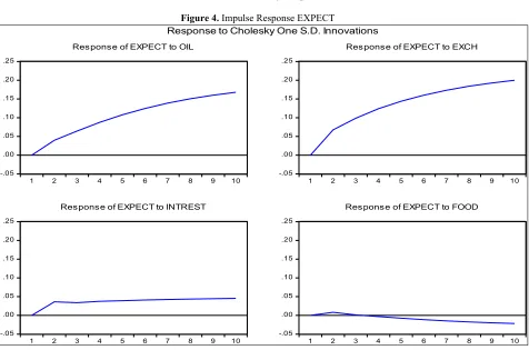
Figure 4. Impulse Response EXPECT
Impulse response functions in Figure 4 show the dynamic response of EXPECT to a one-period standard deviation shock to the innovations of the system and also indicate the directions and persistence of the response to each of the shocks over 10 consecutive periods. For the most part, the impulse response functions have the expected pattern and confirm the results from the short run relationship analysis. Shocks to all the variables are significant although they are not persistent. A one-period standard deviation shock to OIL and EXCH marginally appreciates EXPECT infinitely confirming the positive relationship between the variables as suggested in Equation 1.8. The impulse response results also suggested that a one period standard deviation shock to INTREST marginally appreciates EXPECT by about 3 per cent, but quickly levels off in the second period. Differently, a one period standard deviation shock to FOOD slightly appreciates EXPECT by about 1 per cent but quickly depreciates in the second period to about -3 per cent in the 10th period. The depreciation in expected inflation as a response to a shock
in FOOD confirms the negative relationship between the variables as shown in Equation 1.8.
CONCLUSION AND POLICY IMPLICATIONS
The vector autoregression model was used in this paper to assess the impact of crude oil prices and exchange rates on inflation expectations in South Africa. Monthly time-series data for the period July 2002 to March 2013, obtained from the electronic database of the South African Reserve Bank were used. The data were first examined for unit root using both the ADF and the PP tests and it was observed that the series were all stationary when first differenced, that is, they are integrated of the first order, I(1). The Johansen and Juselius (1990) cointegration test was adopted since variables were I(1). Upon establishing the existence of at least a cointegrating equation, the study used the Vector Error Correction Model (VECM) to disaggregate the short run and long run effects of crude oil prices (OIL), exchange rates (EXCH), interest rates (INTREST) and the cost of food (FOOD) on inflation expectations (EXPECT) in South Africa. The impact of the selected explanatory variables on EXPECT yielded statistically significant results suggesting that OIL and EXCH have a positive relationship with EXPECT while INTREST and FOOD inversely relate with EXPECT. These results are compatible with economic theory and the model used was fit, without any misspecifications because diagnostic checks were also performed in the study. Inferences from this study can therefore be relied on.
-.05 .00 .05 .10 .15 .20 .25
1 2 3 4 5 6 7 8 9 10
Response of EXPECT to OIL
-.05 .00 .05 .10 .15 .20 .25
1 2 3 4 5 6 7 8 9 10
Response of EXPECT to EXCH
-.05 .00 .05 .10 .15 .20 .25
1 2 3 4 5 6 7 8 9 10
Response of EXPECT to INTREST
-.05 .00 .05 .10 .15 .20 .25
1 2 3 4 5 6 7 8 9 10
Response of EXPECT to FOOD
A stable and low inflation together with well-anchored inflation expectations are important to monetary authorities as they help in achieving monetary policy objectives such as economic growth and financial stability. Therefore, inflation expectations significantly influence actual inflation and, thus, the central bank's ability to achieve price stability. Since South Africa has no known oil deposits and depends on imports, a successful inflation targeting would therefore seem to require accurate predictions of the exchange rate. The repo rate instead of targeting only inflation can be used to also anchor the exchange rate since the exchange rate affects inflation expectations and ultimately actual inflation. An appreciating exchange rate can push inflation down thus helping curbing future inflation expectations.
AUTHORS’ INFORMATION
Kin Sibanda is a PhD (Economics) student in the Department of Economics at the University of Fort Hare in South Africa. His research interests include monetary economics, development finance, environmental economics and macroeconomic theory. Mr Sibanda is the corresponding author and can be contacted at: keith08.kin@gmail.com
Progress Hove is a PhD (Logistics) student in the Department of Logistics at the Vaal University of Technology in South Africa. Her research interest includes logistics, supply chain management, business management and transport economics. Miss Hove can be contacted at: proggyhove@gmail.com
Genius Murwirapachena is an Economics Lecturer at the Durban University of Technology, South Africa. His research interests include public economics, environmental economics, labour economics as well as macroeconomics. He can be contacted at: murwiragenius@gmail.com
REFERENCES
Baum, C. F., 2001. The language of choice for time series analysis. Stata Journal, Volume 1, 1-16
Bernanke, C. B. S., 2007. Inflation Expectations and Inflation Forecasting. Speech at the Monetary Economics Workshop of the National Bureau of Economic Research Summer Institute, Cambridge, Massachusetts Bleaney, M., 2001. Exchange rate regime and inflation persistence, international Monetary Fund, 47(3). Celik, T and Akgul, B., 2011. Changes in fuel prices in Turkey: An estimation of inflation effect using VAR
analysis. Journal of Economics and Business, 2, 11-21.
Chisadza, C., Dlamini J., Gupta R and Modise, M., 2013. The impact of oil shocks on the South African economy. Pretoria University department of Economics working paper series.
Curtin, P., 2009. Inflation expectations and empirical tests. New York: Routlegde Taylor and Francis Group. Dickey, D. A. and Fuller, W. A., 1981. Likelihood ratio statistics for autoregressive processes. Econometrica,
Volume 49, pp. 1057-1072
Driver, R and Windram, R., 2007. Public attitudes to inflation and interest rates. Bank of England Quarterly Bulletin, Vol. 47, No. 2, pages 208–23.
Energy Information Administration, 2013. OPEC Revenues: Country Details. www.eia.doe.gov Accessed 16 March 2013.
Gujarati, D.N. 2003. Basic econometrics - 4th edition, New York: McGraw-Hill Inc
Johansen, S., and Juselius. K. 1990. The Full Information Maximum Likelihood Procedure for Inference on Cointegration-with Applications to the Demand for Money. Oxford Bulletin of Economics and Statistics, 52.
Kantor, B and Kavli, H., 2011. Inflation and inflation expectations in South Africa: the observed absence of second round effects. SARB conference.
Marcus, G., 2013. Statement of the Monetary Policy Committee. Issued by the Governor of the South African Reserve Bank, at a meeting of the Monetary Policy Committee (MPC) in Pretoria.
Mboweni, T. T., 2003. Inflation targeting in South Africa. Speech at the BIS/SARB Reserve Management Seminar dinner, South African Reserve Bank, Pretoria, 2 September 2003.
Mohanty, D., 2012. The Importance of Inflation Expectations. Speech at S.P. Jain Institute of Management and Research, Mumbai, 9th November 2012.
Nkomo, J. C., 2006. Crude oil price movements and their impact on South Africa. Energy Research Centre, University of Cape Town Journal of Energy in Southern Africa,17(4) .
Odria, L. R. M., Castillo, P and Rodriguez, G., 2012. Does exchange rate pass through into price changes when inflation targeting scheme is adopted? The Perusian case study between 1994 and 2007. Journal of Macroeconomics, 34, 1154-1166.
Saunders, A., 2004: Macroeconomic policy in South Africa, 1996-2009.[Online]
Available:http://cje.oxfordjournals.org/cgi/interest-rate.in-flation-content//23/6/795[Accessed10 April 2014]
Segal, P., 2011. Oil price shocks and the macro economy. Oxford Review of Economic Policy, 27(1), 169-185. Sinclair, P., 2010. Inflation expectations and empirical tests. New York: Routlegde Taylor and Francis Group. Ueda, K., 2010. Determinants of households’ inflation expectations in Japan and USA. Journal of Japanese and
International Economics, 24(4).
Wakeford, J. J., 2006. The impact of oil price shocks on the South African macroeconomy: History and prospects. SARB Conference.