[NORMAL] Investigations into the thermal comfort and indoor air quality of rooms in low energy homes using a combined heating and ventilation system

(1)

INDOOR AIR QUALITY OF ROOMS IN LOW ENERGY HOMES

USING A COMBINED HEATING AND VENTILATION SYSTEM

A thesis submitted for the degree o f

DOCTOR OF PHILOSOPHY in the

Faculty o f Engineering

UNIVERSITY OF LONDON

by

Patrick Kwaku Ata

February 1997

Department o f Mechanical Engineering University College London

(2)

INFORMATION TO ALL USERS

The quality of this reproduction is dependent upon the quality of the copy submitted.

In the unlikely event that the author did not send a complete manuscript

and there are missing pages, th ese will be noted. Also, if material had to be removed, a note will indicate the deletion.

uest.

ProQuest 10055419

Published by ProQuest LLC(2016). Copyright of the Dissertation is held by the Author.

This work is protected against unauthorized copying under Title 17, United States Code. Microform Edition © ProQuest LLC.

ProQuest LLC

789 East Eisenhower Parkway P.O. Box 1346

(3)

(4)

The objective o f the research was to identify a suitable heating and ventilation system for the provision and control o f thermal comfort in rooms o f fiiture low energy homes. This was to be achieved whilst allowing for the provision o f good indoor air quality (lA Q ) and minimisation o f energy consumption.

The thesis describes the investigations o f individual room airflow and the implications on thermal comfort, indoor air quality and energy consumption. Using a commercial computational fluid dynamics package, numerical simulations were performed to produce airflow patterns and distributions o f temperature and pollutants within a room. A numerical model was validated for use in indoor airflow. The model was used, first o f all, in the identification o f a suitable configuration o f supply and extract air terminal devices, over the expected range o f boundary conditions. Further to this, parametric and sensitivity studies were performed on the proposed system to establish the influence o f the airflow rate, supply air temperature and room specific parameters such as internal heat sources, furniture etc. on the indoor environment. Time dependent variations were considered in order to provide a better understanding o f the transient nature o f the system. The research also included determination o f necessary locations o f sensor/measurement points which provide representative conditions o f the thermal environment in the room.

(5)

I would like to express my gratitude to various parties who have all contributed, in one form or another, to the making and completion o f this thesis.

I am indebted to my supervisor. Dr. K. O. Suen, for his generous help and guidance throughout the project.

I would like to acknowledge the financial and institutional support provided by the Daimler Benz AG through Mr R. Seyer and Dr. Schneider (Daimler Benz Forschungsinstitut, Frankfurt) and Mr Lockl (AEG, Frankfurt).

I would like to express my appreciation to my colleagues in the ‘Control Lab’ who have provided a stimulating and pleasant working environment over the last four years: Alex, Jason, Susana, Habib, Duncan, Szen and Raju — many thanks.

I would like to thank my friends w hose support has been invaluable. In particular I would like to thank Annette Sommer, Yaw Kankam-Boadu, Lesley Lokko, Farhana Malik, Elkin Pianim and Philip Liverpool for their various inputs, direct or otherwise.

(6)

T A BLE O F C O N T E N T S ... I

L IST O F F IG U R E S ... V

LIST O F T A B L E S ...XII

N O M E N C L A T U R E ... XIV

1. INTRODUCTION

1

1.1 A PPL IC A T IO N D O M A IN 1

1. 1. 1 L o w ENERGY HOMES...2

1.1.2 Na t u r a lv s. m e c h a n ic a lv e n t il a t io n...3

1.1.3 De m a n dcontrolledv e n t il a t io n...5

1.1.4 Sp a c eh e a t in g...6

1.2 IN D O O R A m Q U A L IT Y 7 1.2.1 In d o o r AIR POLLUTANTS... 7

O d o u r s... 8

Carbon dioxide (CO ^)... 9

Form aldehyde... 10

W ater vapour... 12

T obacco and Carbon m onoxide (C O )...12

1.2.2 THE OLE AND DECIPOL... 14

1.3 T H E R M A L C O M F O R T ... 15

1.3.1 Th er m alse n sa t io nm e a su r e db y the P M V ... 16

1.3.2 Lo c a ltherm ald isc o m f o r t s... 21

Percentage dissatisfied due to draught... 22

Percentage dissatisfied due to vertical air temperature difference... 23

1.4 IN D O O R A IR F L O W ...24

Experimental investigations... 25

Num erical flo w m o d ellin g ...25

1.5 R E V IE W O F FIN D IN G S O F PR E V IO U S W O R K ... 27

1.5.1 Aird istr ib u tio ns y s t e m s...2 7 C o m m en ts... 30

1.5.2 Th er m alcom fortc o n t r o l...31

C o m m en ts... 35

1.6 O B JE C T IV E S O F THE PR E SE N T R E SE A R C H 36

(7)

2 . I N D O O R A I R F L O W M O D E L L I N G U S I N G

C O M P U T A T I O N A L F L U I D D Y N A M I C S ( C F D ) 40

2.1 FU N D A M E N T A L S O F CFD 41

2.1.1 Governingequationsoffluidf l o w... 41

Conservation o f m ass... 41

Conservation o f momentum... 42

Conservation o f energy...43

Conservation o f chemical species (pollutant concentration)... 44

The general transport equation... 44

2.1.2 Numericalsolutionproceduresofthetransporteq uations... 45

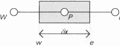
Discretisation using the Finite Volume Method (F V M )... 45

Solution procedures...48

Boundary conditions...49

Numerical considerations... 49

2.2 C FD PR O G R A M A N D M O D E L S A PPLIED IN THIS R E SE A R C H W O R K ... 51

2.2.1 CFD PROGRAM USED: PHOENICS... 51

The pre-processor...51

The solver... 52

The post-processor... 52

2.2.2 Identificationofa suitable airflowmodelfor Indoo r a irflo w 53 Standard k-e turbulence m odel...55

The tw o layer k-e model ( 2 L ) ...56

Lam-Bremhorst k-e turbulence model (L B )... 57

2.2.3 Validation OF A TURBULENCE MODEL... 58

Experimental data...58

Prediction o f cavity airflow using the 2L and LB m o d el... 59

2.2.4 Rooma n d H & V systemsetup/specification... 62

Air supply d evice...62

Grid...63

Simulations... 64

2.2.5 Problem senc o u ntered... 64

3. BOUNDARY CONDITIONS

69 3.1 H E A T T R A N SM ISSIO N T H R O U G H THE R O O M E N V E L O PE 70 3.1.1 Ex t e r n a lclimaticc o n d it io n s...71

Typical winter day, without solar radiation... 71

Typical winter day, with solar radiation... 71

Design day, without solar radiation... 72

3.2 B U IL D IN G F A B R IC ... 72

(8)

3.4 T R A N SIE N T H E A T T R A N SM ISSIO N U SIN G TH E T R A N SFE R

FU N C T IO N M E T H O D ( T F M )... 75

3.4.1 Co n d u c t io n Tr a n sfe r Fu n c tio n s (G IF )...77

CTF O utputs... 80

3.4.2 Weighting FACTORS...81

3.4.3 Spa c ea irt r a n sferfu n c t io n s ( S A I F ) ...82

SATF Outputs...84

Estimated wall surface temperatures... 84

3.5 W A L L SUR FA C E T E M PE R A T U R E V A R IA T IO N S 85 3.5.1 Min im u msu r fa c e t e m p e r a t u r e s... 85

3.5.2 Ma x im u m v a r ia t io n sinsu r fa c et e m p e r a t u r e... 86

3.6 V E R T IC A L T E M PE R A T U R E G R A D IE N T IN THE SIDE W A L L S 89 3.7 A IR FL O W R A T E S ... 91

3.7.1 S p a c e HEATING...91

3.7.2 V e n t i l a t i o n RATES... 92

3.8 O V E R V IE W ... 94

4. CHOICE OF SUPPLY AND EXTRACT AIR TERMINAL

DEVICE (ATD) CONFIGURATION

95 4.1 A T D C O N FIG U R A T IO N S 95 4.2 R O O M C O N F IG U R A T IO N ... 96

4.3 E V A L U A T IO N CRITERIA A N D PR O C E D U R E S 97 4.3.2 CFD OUTPUTS...99

4.3.3 Ev a l u a t io n SCHEME...101

4.4 R A N G E O F IN V E ST IG A T IO N (FLO W R A T E S, SU PPL Y A IR T E M PE R A T U R E S A N D W A L L SU R FA C E T E M PE R A T U R E S) 101 4.5 SIM U L A T IO N S... 102

4.6 R E S U L T S ... 103

4.8 A N A L Y SIS O F THE R E S U L T S... 106

4.8.1 In fl u e n c eof ATD-a r e a / su pply-m o m e n t u mo nt h erm a lc o m fort a n d I A Q ...106

High level supply (Configuration A )... 106

L ow level Supply (Configurations B and D ) ...110

4.8.2 In fl u en c eoflo c a tio no f ATD d ev ic eo ntherm alc o m f o r t...114

4.8.3 Co m p a r iso nofc o n fig u r a tio n s, th erm alco m fo r t, IAQ a n den er g y CONSUMPTION... 115

(9)

4.10 C O N C L U SIO N S... 119

5 . A N A L Y S I S O F T H E P R O P O S E D S Y S T E M 149 5.1 O B JE C T IV E S... 149

5.2 A P P R O A C H ...151

5.3 SIM U L A T IO N S...151

5.4 E V A L U A T IO N ... 154

5.5 PA R A M E T R IC STUDIES O N TH E STA ND AR D CASE 155 5.6 SEN SITIV ITY S T U D IE S ...160

5.6.1 Verticaltemperaturegradients (vtg) inthesidew alls...160

5.6.2 Ob st a c l e s... 163

5.6.3 H e a t SOURCES... 166

Heat sources within the occupied zon e... 166

Heat sources above the occupied z o n e ... 170

5.6.4 Unequalwallsurfacetem peratures... 171

5.6.5 C o ld WINDOW SURFACE... 173

5.6.6 R oom GEOMETRY... 174

5.6.7 Timedependentv a ria tio ns... 176

5.7 L IM IT S O F O PER A TIO N O F TH E H & V E Q U IP M E N T ...180

5.7.1 Verticalairtemperatureg r a d ien t...181

5.7.2 Draught...185

5.8 T H E R M A L C O M FO R T C O N T R O L ... 186

5.8.1 F e a s ib ility o f PM V c o n t r o l ... 186

5.8.2 Sensorlocationsa n dm easurem ents... 187

5.9 D IS C U S S IO N ...191

5.9.1 O v e r v ie w OF THE RESULTS...191

5.9.2 Recommendedcontrolstrategy...194

6 . C O N C L U S I O N S ... 227

A PPE N D IX A I ... 231

A PPE N D IX A 2 ... 232

(10)

LIST OF FIGURES

Chapter 1

Figure 1.1 Degree of dissatisfaction of odour level with outdoor airflow rate... 8

Figure 1.2 Percentage dissatisfied with vertical air temperature difference between heights o f 0.1 m and 1.1m... 23

Chapter 2 Figure 2.1 Grid points and control volume for a one-dimensional field...46

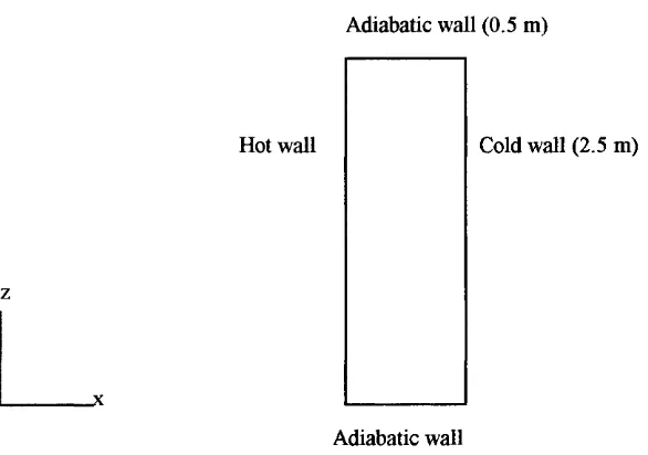
Figure 2.2 Sketch o f the air-filled cavity used in Cheesewright’s (1986) experiment... 59

Figure 2.A1 Velocity vectors in the cavity using the 2L model, grid type 4 ... 66

Figure 2.A2 Velocity vectors in the cavity using the LB model, grid type 3... 66

Figure 2.A3 Velocity distribution in the cavity mid-height using the 2L model, grid types 1 - 4 ...67

Figure 2.A4 Velocity fluctuations in the cavity mid-height using the 2L model, grid types 1 - 4 ... 67

Figure 2.A5 Velocity distribution in the cavity mid-height using the LB model, grid types 1 - 3 ...68

Figure 2.A6 Velocity fluctuations in the cavity mid-height using the LB model, grid types 1 - 3 ...68

Chapter 3 Figure 3.1 Ambient temperature, Jan., Munich... 72

Figure 3.2 Sol-air temperature, 2T^ Jan Munich (South facing wall)... 72

Figure 3.3 Wall configurations in common use... 73

Figure 3.4 Overview o f information inputs and outputs o f transient heat transmission analysis... 76

Figure 3.5 Heat fluxes for walls o f U values o f 0.4... 81

Figure 3.6 Heat fluxes for walls o f U values o f 0.2...81

Figure 3.7 Heat supply rate for walls of U value 0.4... 87

Figure 3.8 Heat supply rate for walls with internal and external insulation, U values 0.4...87

Figure 3.9 Heat supply rate for walls o f U value 0.2... 87

Figure 3.10 Wall temperature variations for wall with U value 0.4...88

Figure 3.11 Temperature variation for wall type 10, with internal (10a) and external insulation (10b), U value 0.4... 88

Figure 3.12 Wall temperature variations for wall with U value 0.2...88

Figure 3.13 Sketch o f flow setup used in the CFD investigation in Chapter 2...90

(11)

Chapter 4

Figure 4. la -f Supply and extract ATD configurations investigated... 96 Figure 4.2 Illustration o f short-circuiting o f the supply air for low ACH of

configuration B ... I l l

Figure 4.A1 PMV and PDv contours of configuration A, 3 ACH, supply velocity

1.1 m/s, supply temperature 42 °C...121 Figure 4.A2 Velocity vectors in plane y = 3 m, configuration A at 3 ACH, supply

velocity 1.1 m/s, supply temperature 42 °C... 122 Figure 4.A3 Enthalpy contours in plane y = 3 m, configuration A at 3 ACH, supply

velocity 1.1 m/s, supply temperature 42 °C... 122 Figure 4.A4 Velocity vectors in plane z = 2.3 m, configuration A at 3 ACH, supply

velocity 1.1 m/s, supply temperature 42 °C... 122 Figure 4.A5 PMV and PDv contours of configuration A, 3 ACH, supply velocity

velocity 0.3 m/s, supply temperature 42 °C... 124 Figure 4.A9 PMV and PDv contours of configuration A, 6 ACH, supply velocity

velocity 2.2 m/s, supply temperature 30 °C... 126 Figure 4.A13 PMV and PDv contours o f configuration A, 6 ACH, supply velocity

velocity 0.6 m/s, supply temperature 30 °C... 128 Figure 4.A16 Velocity vectors in plane z = 2.3 m, configuration A a t...128 Figure 4.A17 PMV and PDv contours of configuration B, 3 ACH, supply velocity

0.44 m/s, supply temperature 42 °C... 129 Figure 4.A18 Velocity vectors in plane y = 3 m, configuration B at 3 ACH, supply

velocity 0.44 m/s, supply temperature 42 °C... 130 Figure 4.A19 Enthalpy contours in plane y = 3 m, configuration B at 3 ACH, supply

velocity 0.44 m/s, supply temperature 42 °C... 130 Figure 4.A20 PMV and PDv contours o f configuration B, 3 ACH, supply velocity

0.3 m/s, supply temperature 42 °C...131 Figure 4.A21 Velocity vectors in plane y = 3 m, configuration B at 3 ACH, supply

(12)

Figure 4.A23 PMV and PDv contours o f configuration B, 6 ACH, supply velocity

0.88 m/s, supply temperature 30 °C... 133 Figure 4.A24 Velocity vectors in plane y = 3 m, configuration B at 6 ACH, supply

velocity 0.88 m/s, supply temperature 30 °C...134 Figure 4.A25 Enthalpy contours in plane y = 3 m, configuration B at 6 ACH, supply

velocity 0.88 m/s, supply temperature 30 °C...134 Figure 4.A26 Velocity vectors in plane z = 1.2 m, configuration B at 6 ACH, supply

velocity 0.88 m/s, supply temperature 30 °C...134 Figure 4.A27 PMV and PDv contours of configuration B, 6 ACH, supply velocity

0.6 m/s, supply temperature 30 °C...135 Figure 4.A28 Velocity vectors in plane y = 3 m, configuration B at 6 ACH, supply

velocity 0.6 m/s, supply temperature 30 °C... 136 Figure 4.A30 Velocity vectors in plane z = 1.2 m, configuration B at 6 ACH, supply

velocity 0.6 m/s, supply temperature 30 °C... 136 Figure 4.A31 PMV and PDv contours of configuration D, 3 ACH, supply velocity

0.3 m/s, supply temperature 42 °C...137 Figure 4.A32 Velocity vectors in plane y = 3 m, configuration D at 3 ACH, supply

velocity 0.3 m/s, supply temperature 42 °C... 138 Figure 4.A33 Enthalpy contours in plane y = 3 m, configuration D at 3 ACH, supply

velocity 0.3 m/s, supply temperature 42 °C... 138 Figure 4.A34 PMV and PDv contours o f configuration D, 3 ACH, supply velocity

velocity 0.34 m/s, supply temperature 30 °C... 144 Figure 4.A43 PMV and PDv contours of configuration B-2, 6 ACH, supply velocity

0.66 m/s, supply temperature 30 °C...145 Figure 4.A44 Velocity vectors in plane y = 3 m, configuration B-2 at 6 ACH, supply

velocity 0.66 m/s, supply temperature 30 °C... 146 Figure 4.A45 Velocity vectors in plane z = 1.2 m, configuration B-2 at 6 ACH, supply

velocity 0.66 m/s, supply temperature 30 °C... 146 Figure 4.A46 Velocity vectors in plane y = 3 m, configuration C at 6 ACH, supply

velocity 0.6 m/s, supply temperature 30 °C... 147 Figure 4.A47 Velocity vectors in plane y = 3 m, configuration E at 6 ACH, supply

(13)

Figure 4.A48 Pollutant concentration contours in plane y = 3 m, configuration A at

3 ACH, supply velocity 0.3 m/s, supply temperature 42 °C...147

Figure 4.A49 Pollutant concentration contours in plane y = 3 m, configuration D at 3 ACH, supply velocity 0.17 m/s, supply temperature 42 °C...148

Chapter 5 Figure 5.1 Variation o f average velocity (over range o f supply air temperatures) with flow rate (ACH)... 157

Figure 5.2 a-d Vertical air temperature variation in the occupied zone o f the ‘standard’ case at 3, 4.5, 6 and 9 ACH... 158

Figure 5.3 Vertical air temperature variation at similar average air temperatures (22.4 °C) at 3, 4.5 and 6 ACH...159

Figure 5.4 Variation o f average pollutant concentration with flow rate (ACH)... 159

Figure 5.5 Vertical air temperatures for cases A, B and C at 3 ACH, supply air temperature 30 °C... 161

Figure 5.6 Vertical air temperature gradients of cases A and C at 3 ACH and various supply air temperatures... 161

Figure 5.7 Vertical air temperatures o f cases A and C at 9 ACH...162

Figure 5.8 Vertical air temperatures with and without obstacles... 164

Figure 5.9 Velocities at the spot values with and without obstacles... 164

Figure 5.10 Turbulence intensities at the spot values with and without obstacles... 165

Figure 5.11 Percentage dissatisfaction due to draught at the spot values with and without obstacles...165

Figure 5.12 Vertical temperatures at 3 ACH with and without unit heat sources...168

Figure 5.13 Vertical temperatures at 9 ACH with and without unit heat sources...168

Figure 5.14 Vertical temperature variation at 4.5 ACH with various heat sources... 168

Figure 5.15 Velocities at the spot values with and without unit heat sources...168

Figure 5.16 Turbulence intensities at the spot values with and without unit heat sources...169

Figure 5.17 Percentage dissatisfaction due to draught at the spot values with and without unit heat sources... 169

Figure 5.18 Percentage dissatisfaction due to draught at the spot values at an average air temperature o f 22.2 °C...169

Figure 5.19 Vertical temperatures with and without high level heat sources...169

Figure 5.20 Vertical air temperatures at various wall surface temperatures (3 ACH)... 172

Figure 5.21 Vertical air temperatures at various wall surface temperatures (4.5 ACH)... 172

Figure 5.22 Vertical temperature variations for a room with a cold window and a standard room...174

Figure 5.23 Average velocities of geometries 1 and 2 ...175

Figure 5.24 Spot values of geometries 1 and 2 at 3 ACH... 175

Figure 5.25 Spot values of geometries 1 and 2 at 6 ACH... 175

Figure 5.26 Vertical air temperatures o f geometries 1 and 2 at 3 ACH...176

Figure 5.27 Vertical air temperatures o f geometries 1 and 2 at 6 ACH...176

Figure 5.28 Vertical air temperatures at times o f 15, 30, 45 mins and the S.S. at 3 ACH .... 178

Figure 5.29 Variation o f pollutant concentration with time at 3 ACH... 178

Figure 5.30 Vertical air temperatures at times o f 15, 30 and the S.S. at 6 ACH ... 179

Figure 5.31 Variation of pollutant concentration with time at 6 ACH... 179

Figure 5.32 Vertical air temperatures at times o f 15, 30 mins and the S.S. at 9 ACH...179

Figure 5.33 Variation of pollutant concentration with time at 9 ACH... 179

(14)

Figure 5.35 Average pollutant concentration with time...180

Figure 5.36 Limits of operation o f supply air temperature... 185

Figure 5.37a-h Temperature ‘measurements’ at specified sensor locations...190

Figure 5.38 Control scheme integrating the use o f SCC... 196

Figure 5.39 SCC control interface and response...198

Figure 5.40 Control scheme integrating the use of SCC, Example 1... 199

Figure 5.41 Control scheme integrating the use o f SCC, Example 2...200

Figure 5.A1 Velocity vectors for the standard case at 3 ACH, supply temperature 35 °C... 202

Figure 5.A4 Velocity vectors for the standard case at 3 ACH, supply temperature 50 °C...203

Figure 5.A6 Velocity vectors for the standard case at 4.5 ACH, supply temperature 25 °C... 204

Figure 5.A7 Velocity vectors for the standard case at 4.5 ACH, supply temperature 30 °C...204

Figure 5.AS Velocity vectors for the standard case at 4.5 ACH, supply temperature 35 °C...204

Figure 5.A l l Velocity vectors for the standard case at 6 ACH, supply temperature 25 °C... 206

Figure 5.A12 Velocity vectors for the standard case at 6 ACH, supply temperature 27.5 °C... 206

Figure 5.A14 Velocity vectors for the standard case at 6 ACH, supply temperature 32.5 °C... 207

Figure 5.A19 Enthalpy contours in the mid-height of the symmetry plane for the standard case at 3 ACH and at supply temperatures of 35-55 °C... 209

Figure 5.A20 Enthalpy contours in the mid-height o f the symmetry plane for the standard case at 4.5 ACH and at supply temperatures of 25-45 °C...209

(15)

Figure 5.A22 Enthalpy contours in the mid-height o f the symmetry plane for the

standard case at 9 ACH and at supply temperatures of 25-35 °C... 210 Figure 5.A23 Velocity vectors for the room without side wall temperature gradients.

Case A, 3 ACH, supply temperature 30 °C... 211 Figure 5.A24 Velocity vectors for the room with side wall temperature gradients.

Case B, 3 ACH, supply temperature 30 °C... 211 Figure 5.A25 Velocity vectors for the room with side wall temperature gradients.

Case C, 3 ACH, supply temperature 30 °C... 211 Figure 5.A26 Velocity vectors for the room without side wall temperature gradients.

Case A, 9 ACH, supply temperature 25 °C... 212 Figure 5.A27 Velocity vectors for the room with side wall temperature gradients.

Case C, 9 ACH, supply temperature 25 °C... 212 Figure 5.A28 Velocity vectors for the room with two obstacles o f dimension

0.4 X 0.4 X 1.4 m^. 9 ACH, supply temperature 25 °C... 213 Figure 5.A29 Velocity vectors for the room with two obstacles of dimension

0.8 X 0.8 X 1.4 m^. 9 ACH, supply temperature 25 °C... 213 Figure 5.A30 Velocity vectors for the room with unit heat sources in the occupied zone,

3 ACH, supply temperature 35 °C...214 Figure 5.A31 Enthalpy contours (y plane) for the room with unit heat sources in the

occupied zone, 3 ACH, supply temperature 35 °C...214 Figure 5.A32 Enthalpy contours (z plane) for the room with unit heat source in the

occupied zone, 3 ACH, supply temperature 35 °C...214 Figure 5.A33 Velocity vectors for the room with unit heat sources in the occupied zone,

4.5 ACH, supply temperature 30 °C... 215 Figure 5.A34 Enthalpy contours (y plane) for the room with unit heat sources in the

occupied zone, 4.5 ACH, supply temperature 30 °C... 215 Figure 5.A35 Enthalpy contours (z plane) for the room with unit heat source in the

occupied zone, 4.5 ACH, supply temperature 30 °C...215 Figure 5.A36 Velocity vectors for the room with unit heat sources in the occupied

zone, 9 ACH, supply temperature 25 °C...216 Figure 5.A37 Enthalpy contours (y plane) for the room with unit heat sources in the

occupied zone, 9 ACH, supply temperature 25 °C...216 Figure 5.A38 Enthalpy contours (z plane) for the room with unit heat source in the

occupied zone, 9 ACH, supply temperature 25 °C...216 Figure 5.A39 Velocity vectors for the room with unit heat sources in the occupied

zone, one heat source moved, 3 ACH, supply temperature 35 °C... 217 Figure 5.A40 Velocity vectors for the room with double heat sources in the occupied

zone, 4.5 ACH, supply temperature 30 °C... 218 Figure 5.A41 Enthalpy contours (y plane) for the room with double heat sources in the

occupied zone, 4.5 ACH, supply temperature 30 °C... 218 Figure 5. A42 Enthalpy contours (z plane) for the room with double heat source in the

occupied zone, 4.5 ACH, supply temperature 30 °C...218 Figure 5.A43 Velocity vectors for the room with a heat source above the occupied zone,

3 ACH, supply temperature 35 °C...219 Figure 5.A44 Enthalpy contours (y plane) for the room with a heat source above the

occupied zone, 3 ACH, supply temperature 35 °C...219 Figure 5.A45 Velocity vectors for the room with a heat source above and within the

occupied zone, 3 ACH, supply temperature 35 °C...220 Figure 5.A46 Enthalpy contours (y plane) for the room with a heat source above and

(16)

Figure 5.A47 Velocity vectors for the room with unequal wall temperatures, Case 1,

3 ACH, supply temperature 42 °C... 221 Figure 5.A48 Velocity vectors for the room with unequal wall temperatures. Case 2,

3 ACH, supply temperature 42 °C... 221 Figure 5.A50 Velocity vectors for the room with unequal wall temperatures, Case 4,

3 ACH, supply temperature 42 °C... 222 Figure 5.A53 Enthalpy contours in mid-height o f the symmetry plane for the room

with unequal wall temperatures. Cases 3 and 4, 4.5 ACH, supply temperature 30 °C. ...223 Figure 5.A54 Velocity vectors for the room with a cold window surface, 6 ACH,

supply temperature 30 °C...223 Figure 5.A55 Enthalpy contours for the room with a cold window surface, 6 ACH

supply temperature 30 °C...223 Figure 5.A56 Velocity vectors for the transient case at 15 mins, 3 ACH, supply

temperature 42 °C... 224 Figure 5.A57 Velocity vectors for the transient case at 30 mins, 3 ACH, supply

temperature 42 °C... 224 Figure 5.A59 Enthalpy contours for the transient case at 15 mins, 3 ACH, supply

temperature 42 °C... 225 Figure 5.A60 Enthalpy contours for the transient case at 30 mins, 3 ACH, supply

(17)

LIST OF TABLES

Chapter 1

Table 1.1 Typical thermal conductivity and air infiltration rates of today’s low energy

homes... 3

Table 1.2 Typical formaldehyde emission rates...11

Table 1.3 Recommended outdoor supply rates...13

Table 1.4 Summary o f TLV concentrations o f the major pollutants or minimum flow rates recommended for acceptable indoor concentration... 14

Table 1.5 Pollution sources for various activities and within buildings... 15

Table 1.6 ASHRAE (1993) seven point thermal sensation scale... 19

Table 1.7 ATD configurations used by Gan (1995)...29

Chapter 2 Table 2.1 Constants used in the Standard high Reynolds number k-e model...56

Table 2.2 Constants used in the Lam-Bremhorst low Reynolds number k-e model...57

Table 2.3 Grid distributions used in simulation o f the buoyant cavity airflow...59

Chapter 3 Table 3.1 Occupancy schedule assumed in the heat transmission analysis... 75

Table 3.2 Categorisation of wall type...78

Table 3.3 CTF coefficients for wall types...79

Table 3.4 Space air transfer function coefficients...83

Table 3.5 Estimated minimum wall temperatures within an hour o f start-up...86

Table 3.6 Estimated maximum differences in surfece temperatures on a typical winter d ay... 89

Table 3.7 Estimated supply air temperatures required to provide space heat demands at various flow rates...92

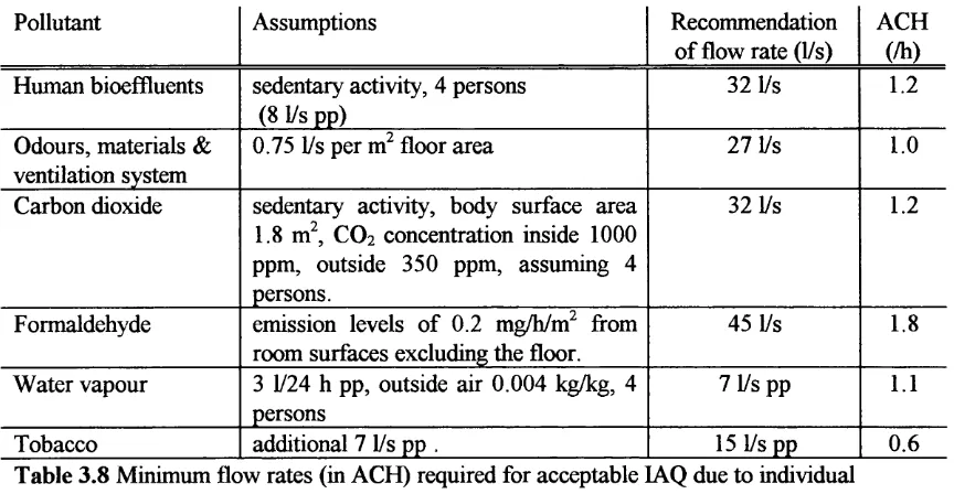
Table 3.8 Minimum flow rates (in ACH) required for acceptable IAQ due to individual pollutants... 93

Table 3.9 Minimum flow rates (in ACH) obtained using the olf... 93

Chapter 4 Table 4.1 Supply and extract ATD centre heights... 97

Table 4.2 Simulations performed to investigate appropriate ATD configuration(s)... 104

Table 4.3 Summary of numerical evaluation data obtained fi'om the simulations hsted in Table 4 .2 ...105

Table 4.4 Numerical evaluation data o f additional cases to obtain similar PM Vs...116

(18)

Table 5.2 Combination o f ACH and supply air temperatures investigated for

simulations o f the standard configuration...156

Table 5.3 Summary o f numerical evaluation results for the standard case...160

Table 5.4 Numerical evaluation values for walls with vertical temperature gradients...163

Table 5.5 Numerical evaluation data for an enclosure with and without internal obstacles. ..165

Table 5.6 Numerical evaluation data for simulations with and without internal heat sources...170

Table 5.7 Wall surfece temperatures (°C), de6ult 19 °C... 171

Table 5.8 Numerical evaluation data for non uniform surface temperatures...173

Table 5.9 Numerical evaluation data for a room with a cold window surface...174

Table 5.10 Numerical evaluation data at varied geometries...176

Table 5.11 Numerical evaluation data for the time dependent cases... 180

Table 5.12 Summary o f observations made in the sensitivity studies on the effect of the RSPs on the local thermal discomforts... 182

Table 5.13 Average PMVs calculated with and without the influence o f velocity... 187

Table 5.14 Locations of sensor ‘measurement’ points... 188

(19)

NOMENCLATURE

A body/wall surface area

A^t,ci constants in LB turbulence model

Aon supply area o f air terminal device

A r Archimedes number

As individual wall surface areas

b„, c„, d„ conduction transfer function coefficients

c,C pollutant concentration

C l 2,3, D, n constants used in the turbulence models

Cp specific heat capacity at constant pressure

E formaldehyde emission rate

fci clothing area factor

f i2,p constants used in the LB turbulence model

g acceleration due to gravity

g„, p„ space air transfer function coefficients

gn* normalised space air transfer function coefficients

he convective heat transfer coefficient

H enthalpy

Id thermal resistance o f clothing

k thermal conductivity, turbulent kinetic energy

Ktot total conductance o f the room envelope

Lm constant used in the 2L turbulence model

m mass flow rate

nif rate o f moisture generation within the building

nig rate o f moisture diffusion through the building fabric

M metabolic activity rate

n summation index, constants

N room air changes per hour

Pa partial water vapour pressure o f the room air

P static pressure

PDiaq percentage dissatisfaction with the indoor air quality

PDv percentage dissatisfied due to draught

PDsr percentage dissatisfied due to vertical air temperature differences

PM V predicted mean vote

q heat load

qe heat gain through a square meter wall section

Qc,e,k r e s,s,w m heat exchange/loss by convection, evaporation, conduction, radiation, respiration, body, mechanical work, metabolic activity.

Rn,k turbulence Reynolds numbers

s individual wall surfaces

source terms in the transport equations

t, T air temperature, air temperature in the room centre

ta air temperature, air temperature in the occupied zone

id surface temperature o f clothing

te sol-air temperature

toff extract-air temperature

(20)

trc constant indoor room air temperature mean radiant temperature

ts wall surface temperatures

T loci. ioc2 air temperature measurements at sensor locations

TI turbulence intensity

w' random fluctuating velocity

Ü mean velocity

U conductance

V local air velocity

Vg CO2 production rate

outdoor air flow rate per o lf

V wwai air velocity measurement at a sensor location on the west wall

V air volume o f room

volume flow rate o f outdoor air

W work rate

X, y, z directions on a cartesian coordinate

yi local distance to a wall

y + Reynolds number in terms o f a non dimensional transverse coordinate

Greek sym bols

Ô time interval

ST temperature difference between fixed heights

A

offset

s dissipation rate o f turbulent kinetic energy

r

diffusion coefficient

laminar viscosity

A turbulent viscosity

<t>

dependent variable

p density

0 Prandtl number, Schmidt number

constants in turbulence models

I summation

X shear stress

6 time

(Ù, specific humidity o f indoor air

Gio specific humidity o f outdoor air

Subscripts

aye

average

e,E

east

i inside

0 outside

(21)

s d standard deviation

w, W west

A bbreviations

ACH air changes per hour

AIC acceptable indoor concentration

ASHRAE American society o f heating refrigeration and air-conditioning engineers

ATD air terminal device

BRE building research establishment

B S British standards

CEN comite european de normalisation

CFD computational fluid dynamics

CHAM concentration heat and momentum

Cl comfort index

CIBSE chartered institute o f building services engineers

CO carbon monoxide

CO2 carbon dioxide

CTF conduction transfer functions

D CV demand controlled ventilation

ECA European collaborative action

FVM finite volume method

H & V heating and ventilation

IAQ indoor air quality

lE A international energy agency

ISO international standards organisation

LB lam bremhorst

LHS left hand side

LW light weight

MAC maximum allowable concentration

PDE partial differential equation

PMV predicted mean vote

PP per person

ppm parts per million

RHS right hand side

RSP room specific parameters

SATF space air transfer functions

SBS sick building syndrome

SCC simple comfort control

s.s.

steady state

TDMA tri-diagonal matrix algorithm

TFM transfer function method

TLV threshold limit values

vtg vertical temperature gradient

WO with obstacle

(22)

In cold climates, the energy consumption o f the built environment's domestic sector constitutes a substantial proportion o f national energy production. Within this, winter space-heating accounts for a significant percentage o f the total energy consumed. Initiated by the energy crisis o f the 7 0 ’s and followed by recognition o f the need to conserve fossil fuel reserves and more recently, the ecological implications o f energy production by fossil fuels - CO2 emissions, there has been a concerted effort to reduce

energy consumption in all sectors. In the building sector, this has led to steadily improving levels o f insulation and air tightness o f the building envelope. Greater air tightness, whilst resulting in reductions in fortuitous air infiltration, and therefore heat losses, also resulted in high concentrations o f indoor air pollutants. This brought about the need for some form o f ventilation system to provide outside/ffesh air to attain or maintain satisfactory indoor air pollutant concentrations. These ventilation systems resulted in additional and inevitable heat losses (known as the ventilation losses) in the provision o f cold outside air (during winter) and extraction o f warm room air. As building insulation levels were fiarther improved, the ventilation losses constituted more significant proportions o f the total heat loss. In recent years, attempts to minimise these losses have seen reductions in outside air supply rates. This era, not coincidentally, has been synonymous with the onset o f the term ‘sick building syndrome’ (SB S). SBS refers to a host o f indoor air quality related complaints which include the sensation o f stuffy and stale air, irritation o f mucous membranes and eyes, headaches, lethargy and so forth. Consequently, the impact o f the indoor air quality (IAQ) on the health and productivity o f the occupants has taken on greater importance, prompting extensive research activities into the causes and implications o f poor IAQ. These studies have primarily addressed the following areas: the identification o f the sources o f indoor air pollution, ventilation rates required to achieve comfortable and healthy indoor environments for extended occupancy and the influence o f the air distribution systems.

(23)

levels o f IAQ and thermal comfort in a room is thus an interdependent process, with a common variable: the air movement. This triangulation o f air movement, IAQ and

thermal comfort, together with the implicit energy implications, is the subject o f this research, in the application domain defined below.

1.1 Application domain

The application domain o f this research is in the heating and ventilation o f low energy homes, located in the temperate climate o f mid European countries. These will be air tight buildings with high standards o f thermal insulation. The study will focus on a combined heating and ventilation system with individual room conditioning and control. The system is to operate intermittently, providing ventilation (outside air) along demand controlled principles, (i.e. the supply o f outside air should satisfy requirements at any given moment). The concept o f comfort control o f the thermal environment as opposed to temperature control is to be assessed.

Reasons for the choice o f ventilation and heating system and mode o f operation will be highlighted in the following sections. These sections include a brief outline o f the current status in the three broad fields which affect this investigation, namely the indoor air quality (IAQ), thermal comfort and air distribution systems. Within these sections, relevant data and mathematical expressions will be identified which were used in the course o f the study. All mathematical expressions listed in this chapter will be used in subsequent chapters. Following the outline o f the three fields, the chapter proceeds to review a number o f recent studies which had a bearing on this research. This is followed by the definition o f the objectives and methodology o f this research.

1.1.1 Low energy homes

(24)

transition from low energy to passive homes is often accompanied by the introduction o f heat recovery devices (e.g. air-to-air heat exchangers and exhaust-air heat pumps) and the use o f alternative energy (or heat) sources, such as solar and geothermal energy sources. The use o f the term low energy home, within this study, refers to buildings with insulation standards o f 0.4 W/m^K or lower, i.e. all three levels in Table 1.1. The implications o f the building insulation and air tightness level on the selection o f heating and ventilation systems is discussed below.

U value o f the building infiltration across the

envelope room envelope

U (W W K) ACH (/h)

low energy homes 0.4 0.5

super insulated homes 0.2 0.35

passive homes 0.1 0.25

Table 1.1 Typical thermal conductivity and air infiltration rates of today’s low energy homes (Infiltration rate is usually o f the order of 1/20* o f the measured air change rate at 50 Pa.

Liddament, 1986)

1.1.2 Natural vs. mechanical ventilation

Natural ventilation is the provision o f outdoor air into a space via openings within the

building fabric as a result o f pressure differences which are caused by wind and stack effects. The stack effect arises from the differences in air temperature and therefore density causing pressure gradients both inside and outside the building. When the inside air temperature is greater than the outside air temperature, colder outside air enters the building through low level openings and warm air escapes at high levels. Natural ventilation may be provided by various strategies;

• ventilation through windows

• ventilation through purpose-provided openings (vents)

(25)

than mechanical systems, these are subject to a major drawback: the inherent uncontrollability due to the unpredictable nature o f wind pressures and temperature differences. The need to conserve energy and avoid indoor air quality problems has seen natural ventilation evolve from arguably its most basic form: infiltration through cracks and gaps in the building envelope. Greater control has been achieved by the reduction o f adventitious infiltration and the provision o f windows and vents which are controlled by the occupants. In addition, the stack effect has been used in buoyancy driven exhaust systems, with outside air provided through purpose built openings. Further improvements {Knoll, 1992) have seen the development o f controllable air inlets such as trickle vents, se lf regulating inlets (by temperature or pressure) and

humidity controlled inlets which are combined with a buoyancy driven exhaust system.

The latter have found applications in colder climates, but still encounter practical difficulties in the modulation o f flow rates, due to their dependence on the climatic conditions. Where good control is required, the tendency is to employ mechanical ventilation systems.

Mechanical ventilation implies the use o f one or more fans to achieve one o f the

following:

• mechanical supply o f outside air • mechanical extraction o f room air

• a combination o f the above (balanced system)

Supply-only or extract-only mechanical ventilation essentially operate on the principle o f over and under pressurisation o f the room, with the resulting exfiltration/infiltration o f air by natural means. These exfiltration/infiltration air routes may be through cracks or gaps in the building fabric or through purpose built openings. Both o f these systems, however, suffer from a number o f drawbacks:

a) difficulties in precise control

b) difficulties in controlling the flow distribution in the room, and

(26)

& extract) should be used for close control o f lA Q by good distribution and mixing o f the supply air and o f the flow rates. These systems allow recirculation o f room air and the incorporation o f filters and heat recovery devices.

1.1.3 Demand controlled ventilation

Demand controlled ventilation (DCV) refers to the provision o f appropriate quantities

o f outdoor air according to the needs and demands at the time. This concept was introduced to reduce energy consumption while maintaining good lAQ. This is achieved by avoiding unnecessary continuously high outdoor air supply rates. These systems vary in complexity from the application o f simple devices such as timers, to the use o f sensors for the evaluation o f the lAQ, occupancy detection etc.

The concept o f D C V is in itself nothing new e.g. providing ventilation during occupancy by the use o f timers or manual activation o f the system. Advances in technology however, both in communication (e.g. network/bus systems) and instrumentation (e.g. measuring instruments/sensors) give a new meaning to the concept o f D C V today. In today’s use, DCV refers to the provision o f sufficient rates o f outdoor air during occupancy, to meet the fluctuating requirements for satisfactory LAQ. This is to provide optimisation between the demands for good lA Q and the energy o f the ventilation system.

The application o f D C V systems is currently under assessment in several studies

(Liddament, 1994). These studies address the necessary measurements to evaluate the

lAQ, the identification o f threshold limit values (TLVs) o f individual pollutants for acceptable lA Q and the development o f sensors to measure pollutant concentrations. D C V systems currently being evaluated include the use o f CO2, relative humidity and

(27)

possible range o f flow rates for DCV operation, the major pollutants will be identified

together with the necessary ventilation rates to achieve satisfactory concentrations o f

these.

1.1.4 Space heating

In most o f the Scandinavian countries, new housing is equipped with balanced

mechanical ventilation systems with heat recovery devices (air-to-air heat exchangers

or air-to-air/water heat pumps) which also provide space heating using air as the heat

transport medium. In more moderate climates (mid-Europe) there is a similar trend

with increasing thermal insulation and tightness o f the building envelope.

The presence o f a balanced ventilation system (with its associated components e.g.

fans, ducts, dampers etc.) makes the use o f an air heating system an attractive and

economically viable option, in particular in terms o f initial cost. The increasing supply

rates o f outside air with building tightness, have resulted in greater volumes o f air

movement and had implications on fan sizing, duct sizing and the energy consumed in

the distribution process. Simultaneous in thermal insulation and space heat

requirement have meant reductions in air quantities required in the provision o f the

space heat requirement. The greater the reduction in space heat requirement, the closer

these two flow rates converge. It has thus become economical both from the

perspective o f initial cost and operating cost to integrate the heating and ventilation

into the same distribution system

The configuration o f the heating and ventilation systems and choice o f primary heat

source could have implications on the most efficient mode o f operation o f the systems

i.e. optimisation in flow rates and supply air temperature. For example with the

availability o f low grade heat sources, operation at increased flow rates could be more

economical despite the higher fan costs. Evaluation o f the relative economies o f

operation, in a similar manner to the use o f DC Vs is beyond the scope o f this

investigation Some consideration though will be given to this in the recommendation

o f a control strategy for the energy efficient provision o f thermal comfort and lAQ in a

(28)

A person’s perception o f indoor air quality is subjective, mainly on the basis o f an

individual's sensation to various odours. This is acceptable for most organic

substances, which are olfactory stimuli. In these cases, the human olfactory system is

superior to most measuring instruments. Inorganic substances however, including

harmful pollutants such as carbon monoxide, cannot be perceived even at high

concentrations. Good indoor air quality thus requires fresh air supply rates to dilute

odours and maintain harmful pollutants within healthy levels. O utdoorlair flow rates

for human respiration are between 0.1-0.9 1/s, depending on metabolic activity rate.

These requirements fall well within the demands for pollutant dilution from for

example human bioeffluents and need not be taken into consideration.

Two approaches will be identified to determine a possible range o f flow rates required

for ventilation purposes:

a) identification o f the major indoor air pollutants and the minimum outdoor airflow

rates required in order not to exceed threshold limit values (TLVs) for acceptable

indoor concentrations, and

b) the use o f two new units developed by Fanger (1988), the o lf and the decipol

1.2.1 Indoor air pollutants

Comprehensive reviews o f research into common indoor pollutants and the ventilation

rates required to control pollutant levels within acceptable limits are given in various

annexes o f the lEAs energy conservation in buildings and community systems

programme, Haherda & Trepte (1989), Raatschen (1989), and Limb (1994) and also

hy Awbi (1991). These publications are the main data sources in the following sections

on individual pollutants and corresponding minimum ventilation rates required. Where

specific references are quoted from these, they are accompanied by superscripts \ ^

and , representing the order o f appearance above.

(29)

Odours

The main sources o f odours in habitable rooms have, until recently, been assumed to be due mainly to the occupants. Recent studies contradict this assumption. These studies have identified sources such as building materials, furnishings and the ventilation system to produce greater concentrations o f odorous pollutants, when combined, than human bioeffuents. It is now widely accepted that other odour sources are at least as significant as those from human bioeffluents. This position is reflected in the revisions o f the proposed new standards in the US in ASHRAE standard 62 (1996) and in Europe in Comite Européen de Normalisation (GEN) pre-standard prEN V 1752

{Fanger, 1996). These new standards specify minimum flow rates to cater for odour

dilution from persons as well as fi'om materials. The proposed ASHRAE standard is currently restricted to commercial buildings and does not apply to dwellings.

Laboratory and field study results have correlated a persons degree o f dissatisfaction (based on a large sample o f persons) with body odour from a sedentary person against outdoor air supply rate. For unadapted persons, freshly entering the space, the degree o f dissatisfaction with outdoor airflow rate may be estimated from Figure 1.1^.

ASHRAE standard 62 (1989) recommends the use o f similar limits o f acceptable

dissatisfaction level (20%) due to indoor air pollution as those used in the ISO

standard 7730 (1993) for thermal comfort. This results in the recommendation o f

outdoor air flow rates o f 8 1/s per person (fi'om Figure 1.1).

Body Odour 35

3 0

-20 I/s • person

10 15

5

0

Ventilation rate

(30)

partially due to the large variations found in materials, furnishings, and systems between buildings. Average building stock has been estimated (ECA, 1994) to require approximately 0.75 1/s per square metre o f floor area for living rooms and bedrooms to achieve acceptable odour levels.

Carbon dioxide (CO^)

The rate o f production o f CO^ ( , 1/s) by human respiration is related to metabolic

rate by the following expression.

V = 4 x l O W . y 4

^ 1.1

where

M = metabolic rate (W/m^)

A = body surface area (m^)

The maximum allowable concentrations (MAC) for 8 hour occupation recommended

in various standards is 5000 ppm. For acceptable indoor concentrations (AIC), the recommendation^ in various countries is to keep the concentrations to minimum levels o f between 800 and 1500 ppm. Jannsen (1994) and his associates studied the response o f school children to CO^ controlled ventilation. They found an acceptance o f the environment at CO^ levels o f 1 0 0 0 ppm with a rise in discomfort at 1600 ppm with

complaints o f stuffy, more stagnant and warmer air and the sensation o f warmer hands and feet with respect to the rest o f the body. Although CO^ is not poisonous to humans below a concentration o f 50000 ppm, physiological effects have been observed at concentrations above 10000 ppm. It is not known whether these are harmful in the long term.

The CO2 concentration in outside air is approximately 350 ppm, with minor increases

year on year. The variation o f the environmental concentration o f CO^ rarely exceeds 150 ppm. This relatively minor variation in CO^ concentration combined with the large

percentage o f CO2 in expired air (4.4 % by volume) and the fact CO2 cannot be filtered

(31)

Assuming perfect mixing, outdoor air flow rates (V^ l/s) can be estimated from a steady state mass balance;

where

v„

l - C ^

= internal generation rate o f CO^ (1/s)

Co = outdoor concentration o f CO^ (ppm) C, = indoor concentration o f CO^ (ppm)

This expression will be used in the estimation o f required air flow rates to prevent indoor CO^ concentrations from exceeding the recommended hmit ( 1 0 0 0 ppm) for

acceptable indoor concentration.

Formaldehyde

Formaldehyde exists extensively in today’s environments. It is present in building materials such as compressed w ood boards, plastic foam insulation, bonding and laminating agents, adhesives, as well as in packaging products, toiletries and cosmetics. Combustion appliances and tobacco smoke also generate appreciable amounts. At low concentrations, formaldehyde may cause discomfort due to odours or irritations to the eyes, nose, throat and related symptoms such as headaches. In higher concentrations, tests on animals suggest this may pose carcinogenic risks to humans. M ost current ventilation standards allow MAC o f formaldehyde o f 1 ppm and recommend AICs o f 0.1 ppm. It is however, not currently proven that health risks do not exist at the AIC level, particularly over long term exposures. Currently, the health implications at 0. 1

ppm are suspected to be minimal or at least tolerable. Various studies (Cain et al,

1986) have found differing human sensitivity levels to the detection o f formaldehyde, ranging from 0.03 ppm to 1 . 0 0 ppm. Tests have also shown decreasing irritation levels

(32)

Studies in the UK and Germany have recommended minimum air changes per hour (ACH) o f between 0.5 and 0.8, thus maintaining concentrations within AIC levels. However, results (Walsh et al, 1984'^) from an energy efficient house in the U SA obtained formaldehyde concentrations well in excess o f the 0 . 1 ppm threshold.

Concentrations o f up to 0.35 ppm were obtained at ACH o f 0.83. These high formaldehyde concentrations were attributed to the insulation materials.

Typical formaldehyde emission rates o f today’s materials are given in Table 1.2. Its concentration in room air is dependent on various factors: the area o f the emitting surface, total air volume, air change rate, and other parameters such as temperature, humidity and age o f the formaldehyde source. Where no formaldehyde sinks are present within a room (i.e. assuming unsupressed emission), the room concentration (C, ppm) may be estimated by the expression'll

p - N - V j 3

where

A = area o f emitting surface, (m^)

E = net emission rate, (mg/hm^)

p = density, (kg/m^)

N = air change rate, (/h)

V = air volume o f room (m^)

Equation 1.3 may be used together with the data in Table 1.2 in the estimation o f necessary outdoor air flow rates to maintain formaldehyde concentrations within AIC levels (0 . 1 ppm).

Material Emission Rate, E

(mg/hm^)

woodchip boards 0 .4 6 -1 .6 9

compressed cellulose boards (hardboards) 0.17-0.51

plasterboards 0 -0 .1 3

wallpapers 0 -0 .2 8

carpets 0

curtains 0

(33)

Water vapour

High moisture levels may have an impact on the occupants comfort and health. Low humidity levels are believed to contribute to increased risks o f infection, whereas high humidity levels may result in condensation within the room. Condensation, when combined with inadequate ventilation, may cause musty smells as a result o f mould and fungal growth. As well as having an adverse effect on the occupants health, long term condensation often leads to structural damage to walls and materials within the room.

Relative humidities o f between 30-70 % are recommended in habitable rooms. High moisture levels can be restricted by adequate ventilation rates, due to relatively dry outdoor air, particularly during cold seasons. Moisture production within a dwelling is mainly from occupants and their activities. Assuming well zoned buildings, moisture production in habitable rooms would be due mainly to the emission from the occupants o f approximately 2-3 1 per 24 hours for active occupants (Building Research Establishment ). Allowances may be made for activities such as meals and some spill over from other higher production zones. Assuming perfect mixing o f the indoor air, the outdoor airflow rate (V^, m^/s ) required to attain specified indoor air moisture levels (or relative humidity) can be estimated from a moisture balance for the zone;

where

nig = rate o f moisture generation within the building (kg/s)

n if = rate o f moisture diffusion through the building fabric (kg/s)

Po = density o f outdoor air (kg/m^)

G). = Specific humidity o f indoor air (kg/k g)

co^ = specific humidity o f outdoor air (kg/kg)

Tobacco and Carbon monoxide (CO)