Improving clustering performance
using independent component analysis
and unsupervised feature learning
Eren Gultepe
*and Masoud Makrehchi
Abstract
Objective: To provide a parsimonious clustering pipeline that provides comparable performance to deep learning-based clustering methods, but without using deep learning algorithms, such as autoencoders.
Materials and methods: Clustering was performed on six benchmark datasets, consisting of five image datasets used in object, face, digit recognition tasks (COIL20, COIL100, CMU-PIE, USPS, and MNIST) and one text document dataset (REUTERS-10K) used in topic recognition. K-means, spectral clustering, Graph Regularized Non-nega-tive Matrix Factorization, and K-means with principal components analysis algorithms were used for clustering. For each clustering algorithm, blind source separation (BSS) using Independent Component Analysis (ICA) was applied. Unsupervised feature learn-ing (UFL) uslearn-ing reconstruction cost ICA (RICA) and sparse filterlearn-ing (SFT) was also per-formed for feature extraction prior to the cluster algorithms. Clustering performance was assessed using the normalized mutual information and unsupervised clustering accuracy metrics.
Results: Performing, ICA BSS after the initial matrix factorization step provided the maximum clustering performance in four out of six datasets (COIL100, CMU-PIE, MNIST, and REUTERS-10K). Applying UFL as an initial processing component helped to provide the maximum performance in three out of six datasets (USPS, COIL20, and COIL100). Compared to state-of-the-art non-deep learning clustering methods, ICA BSS and/ or UFL with graph-based clustering algorithms outperformed all other methods. With respect to deep learning-based clustering algorithms, the new methodology pre-sented here obtained the following rankings: COIL20, 2nd out of 5; COIL100, 2nd out of 5; CMU-PIE, 2nd out of 5; USPS, 3rd out of 9; MNIST, 8th out of 15; and REUTERS-10K, 4th out of 5.
Discussion: By using only ICA BSS and UFL using RICA and SFT, clustering accuracy that is better or on par with many deep learning-based clustering algorithms was achieved. For instance, by applying ICA BSS to spectral clustering on the MNIST dataset, we obtained an accuracy of 0.882. This is better than the well-known Deep Embedded Clustering algorithm that had obtained an accuracy of 0.818 using stacked denoising autoencoders in its model.
Open Access
© The Author(s) 2018. This article is distributed under the terms of the Creative Commons Attribution 4.0 International License (http://creativecommons.org/licenses/by/4.0/), which permits unrestricted use, distribution, and reproduction in any medium, provided you give appropriate credit to the original author(s) and the source, provide a link to the Creative Commons license, and indicate if changes were made.
RESEARCH
Conclusion: Using the new clustering pipeline presented here, effective clustering performance can be obtained without employing deep clustering algorithms and their accompanying hyper-parameter tuning procedure.
Keywords: Spectral clustering, Independent component analysis, Sparse filtering, Reconstruction ICA, Unsupervised feature learning, Clustering, Graph Regularized Non-negative Matrix Factorization
Introduction
Grouping observed data into cohesive clusters without any prior label information is an important task. Especially, in the era of big-data, in which very large and complex amounts of data from various platforms are collected, such as image content from Facebook or vital signs and genomic sequences measured from patients in hospi-tals [1]. Often, these data are not labeled and a significant undertaking is typically required (usually by individuals with domain knowledge). Even in simple tasks, such as labeling images or video data can require thousands of hours [2, 3]. Therefore, using the unsupervised learning technique of cluster analysis can aide in the process of providing labels to observed data [4].
Classical clustering algorithms
Classical clustering algorithms used for analysis are K-means [5], Gaussian Mixture Models [6], and hierarchical clustering [4], all of which are based on using a distance measure to assess the similarity of observations. The choice for distance measure is typically data dependent. For instance, in image data, the similarity between pixels can be represented by the Euclidean distance, where as in text documents cosine dis-tance matrix is typically used [7]. Moreover, appropriate feature representation of the observations is even more critical in order to obtain correct clusters of the data [8], since improved features provide a better representative similarity matrix.
Deep learning‑based clustering
Early approaches for learning the appropriate feature space in clustering algorithms implemented deep autoencoders (DAEs) [9]. Song et al. [10] used DAEs to directly learn the data representations and cluster centers. Huang et al. [11] employed a DAE with locality and sparsity preserving constraints, which is followed by a K-means to obtain the cluster memberships. A more recent and popular approach by Xie et al. [8] learned the feature space and cluster membership directly using a stacked denois-ing autoencoder [12]. Following Xie et al. [8], there have been many studies propos-ing deep clusterpropos-ing algorithms to learn the feature space and cluster membership simultaneously using some form of an autoencoder [13–15]. A departure from the autoencoder framework was demonstrated by Yang et al. [16], who used recurrent and convolutional neural networks with agglomerative (hierarchical) clustering.
Spectral clustering
as spectral decomposition) of the Laplacian matrix [19]. Spectral clustering usually performs better than K-means and the aforementioned classical algorithms due to its ability to cluster non-spherical data [4]. A key issue in spectral clustering is to solve the multiclass clustering problem. This is accomplished by representing the graph Laplacian in terms of k eigenvectors, k being the number classes [20]. Then, either K-means clustering [18], exhaustive search [17], or discretization [21] is applied to this lower dimensional representation of the Laplacian to determine the final cluster memberships. Recently, autoencoders have been applied on the Laplacian to obtain the spectral embedding provided by the eigenvectors [22]. Another approach has been to use a deep learning network that directly maps the input data into the lower dimensional eigenvector representation, which is then followed by a simple clustering algorithm [23].
Research aim
The drawback of deep learning methods is that they tend to have many hyper-parame-ters, such as learning rates, momentum, sparsity paramehyper-parame-ters, and number of features and layers [14, 24, 25]. All of which can make deep learning models difficult to train, since hyper-parameters can severely effect performance [24]. Typically, choosing the correct hyper-parameters requires expertise and ad hoc selection [14, 25]. However, the high degree of complexity in implementing deep learning-based algorithms [24] may be a lim-iting factor of their application in non-computer science based research fields. To have real-world applicability, clustering applications need to have as few hyper-parameters as possible [14].
In this study, the aim is to provide a parsimonious and accessible clustering processing scheme that incorporates deep learning-style feature extraction, but without the complex hyper-parameter tuning procedure. The goal is to bridge the gap between deep learning-based clustering methods and widely available standard clustering techniques. This is accomplished by using two procedures. First, we improve the clustering accuracy of stand-ard clustering algorithms by applying independent component analysis (ICA) [26] blind source separation (BSS) after the initial matrix factorization step in principal component analysis (PCA) and graph-based clustering algorithms. Second, we improve the features used for constructing the distance matrix in graph-based clustering techniques by perform-ing feature extraction usperform-ing deep learnperform-ing-inspired feature learnperform-ing techniques. Prior to any clustering algorithm, we implement the unsupervised feature learning (UFL) algorithms of ICA with reconstruction cost (RICA) [27] and sparse filtering (SFT) [28], both of which have only one tunable hyper-parameter—the number features [28].
By implementing these two procedures we demonstrate that effective clustering perfor-mance that is on par with more complex deep learning clustering models can be achieved. Thus, the clustering methodologies provided herein are designed to be simple to implement and train in different data applications.
Materials and methods
and (4) K-means clustering. In the following, the datasets are first described and then the four components are introduced.
Data
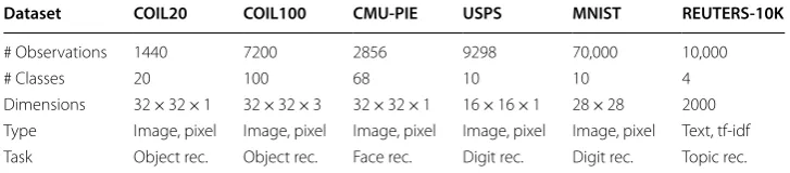
In order to test the generalizability of the proposed clustering methodology, six bench-mark datasets are used for the experiments; five image datasets and one text dataset (see Table 1 for a summary of datasets).
Feature extraction and unsupervised feature learning
For all image datasets, L2-normalization (each observation input feature vec-tor is transformed to have a unit norm) was performed on the image pixel intensi-ties (each observation input feature vector is transformed to have a unit norm).
Fig. 1 Pipeline for processing. Each of the components contains the options available for implementation. The simplest processing pipeline to obtain clustering results consists of a L2-normalization on the data,
followed by K-means clustering. The processing stream with the most components would consist: (1) L2-normalization followed by UFL using either RICA or SFT; (2) similarity graph construction; (3) GNMF or
spectral decomposition followed by ICA blind source separation; and (4) K-means clustering
Table 1 Description of datasets used in experiments
COIL20: grayscale images for object recognition dataset containing 20 objects positioned at 72 different angles [29]. COIL100: RGB images of 100 objects at 72 different poses [29]. The images were downsampled to 32 × 32 pixels from the original 128 × 128 pixels to facilitate analysis for unsupervised feature learning [24]. CMU-PIE: grayscale images of 68 human faces with 4 different poses [30]. USPS: grayscale images of handwritten digits (0–9) from the USPS postal service [31]. MNIST: grayscales images of handwritten digits (0–9) obtained from NIST [32]. REUTERS-10K: A Reuters news service dataset containing text documents in English that is used for topic recognition, which was processed according to Xie et al. [8]. The term frequency–inverse document frequency (tf-idf) [33] feature matrix was computed, using the 2000 most frequent words
Dataset COIL20 COIL100 CMU‑PIE USPS MNIST REUTERS‑10K
L2-normalization has been empirically shown to improve clustering performance [16]. The L2-normalization was not performed directly on the raw input data of the REUTERS-10K text document dataset because for text documents, the tf-idf matrix [33] was constructed. Nonetheless, each observation still has unit norm [7]. At this stage, the normalized image and text data can be used as input into the clustering algorithms.
Following normalization, the feature extraction component diverges into two separate stages. The first stage is performed by principal components analysis (PCA), which is a linear method of feature extraction and data compression [34]. PCA is performed on the normalized datasets by using singular value decomposition (SVD). SVD has been shown to be successful in topic recognition for text documents (Latent Semantic Indexing [35]) and face recognition in images (using eigendecomposition in Eigenfaces [36]). SVD pro-vides a good baseline for comparison to more complex feature extraction algorithms [7, 37]. To determine the number of principal components, we used spectral clustering as our inspiration. In spectral clustering, the number eigenvectors used to embed the graph Laplacian is set to the number of clusters expected in the observed/input data. The goal is to embed the signal that is unique to each class into a vector. Thus, in our processing pipeline the number of principal components extracted is set to the number of classes in each dataset, as in spectral clustering [19]. Then the principal components obtained from PCA are used in K-means clustering. PCA with K-means clustering has been used in other studies as well, such as in Cai et al. [7]. However, in Cai et al. [7], the number of principal components is not limited to the number of classes, as in our processing. Rather, the full dimensionality of the original input data is preserved. For example in the CMU-PIE dataset, for the pipeline proposed in our study, 68 principal components are extracted, whereas in [7] 32 × 32 = 1024 principal components are extracted.
After PCA is applied, blind source separation (BSS) can be applied to the extracted components. BSS is the problem of resolving the mixed signal sources, without know-ing the nature of the mixture [38, 39]. ICA is mathematical model of BSS, where the mixed signals are separated into their original sources. This is accomplished by determining the mixing matrix that the maximizes non-Gaussianity and minimizes the mutual information [26]. ICA has been shown to successfully separate source sig-nals into biological meaningful sigsig-nals in electroencephalography (EEG) [40, 41] and functional magnetic resonance imaging (fMRI) data [42, 43]. In our pipeline, ICA is applied to the components obtained by PCA, with the goal to provide more salient embedding vectors to the K-means clustering algorithm. In a recent study by Nasci-mento et al. [44] in 2017, without any PCA dimension reduction, applied ICA directly to the input data prior to hierarchical clustering. However, ICA following PCA has been shown to be more effective at separating the source signals [45]. In our study, the popular FastICA algorithm is used for the application of ICA [46].
A disadvantage of deep neural networks such as autoencoders is their parameter complexity during training [24]. To overcome this complexity, RICA and SFT rithms have been used as substitutes for the feature learning algorithm. These algo-rithms have greatly reduced the number of parameters needed to train an effective model, thus decreasing training time [27, 28]. Both algorithms have only one hyper-parameter, which is the number of features or hidden nodes that need to be learned for proper feature extraction. A summary of RICA [27] and SFT [28] is given below, where X=
xij
∈Rq×s is the input data (with q as the of # observations and s as the # of
fea-tures in a random image patch) and W=wij
∈RK×N is the weight matrix (with K as the # of learned features and N as the # of input features):
Reconstruction ICA
RICA relaxes the orthonormal constraint of ICA to learn an over-complete feature representation. Over-complete features are more robust to noise, sparse, and may cap-ture the underlying struccap-ture of the data better [47]. The RICA algorithm minimizes W using the following objective function, 1
2
WTWx−x
2
2+�Wx� , where λ is a sparsity parameter.
Sparse filtering
SFT directly learns the kth feature fk of the data by L1-minimization, without ever mode-ling the data itself. The feature fk for the ith input x(i) is defined by the soft absolute func-tion fk =
(wT
kx(i))2+ ∈ where ∊= 10−8. The feature fk is L2-normalized first by the
rows and then the columns. Then L1-minimization is performed following the normali-zation steps to ensure equally distributed sparse feature activation.
The second stage of UFL feature extraction is only applied to the image datasets. This is due to the 2D image patch extraction process that is required to implement RICA and SFT [27, 28, 48]. A detailed discussion about how features are extracted and convolved to represent a new feature space can be found in [24, 48, 49].
In summary, there are three types of feature extraction streams for the input data: (1) L2-normalization of the input features, (2) using the L2-normalized data, PCA feature extraction with the added option of ICA BSS, and (3) unsupervised feature learning with RICA or SFT using the L2-normalized features. At this stage, K-means clustering can be directly applied to each of the three types of feature representations, without using any of the graph-based clustering techniques described in the subsequent subsection.
Graph embedding and clustering
After the feature representation of the input data is finalized, the graph embedding procedure can be performed on the new representations of the data. This is a two-step process in which the similarity graph is first constructed and then followed by a matrix factorization step. Once the matrix factorization is obtained, clustering can be performed.
s
xi,xj
= exp
−xi − xj
2 /2σ2
, all pairwise similarities among the observations
X= xij
∈Rm×n (where m is the # of observations and n is the # of input features) are
computed, controlled by the scaling factor σ. Using the similarities S=sij
∈Rm×m (where m is the # of observations) and the k-nearest neighbor (kNN) criterion, the simi-larity graph, otherwise known as the weighted adjacency matrix W, is constructed [19]. Essentially, the kNN criterion simplifies the similarity matrix to a sparse matrix where each observation is connected to only its k-nearest neighbors and all other entries are set to 0.
To perform clustering using the similarity graph W, it needs to be represented by k eigenvectors or basis vectors by way of matrix factorization [7]. One method to accom-plish this is through the standard spectral clustering algorithm [19]. In this study, the two popular spectral clustering algorithms, both of which require the construction of the normalized graph Laplacian, are used. The unnormalized graph Laplacian is defined as L=D−W, where D=dij∈Rm×m (where m is the # of observations) is the
diago-nal degree matrix with diagodiago-nal elements set to dii=mi=1wij and all other entries set to 0. The first version of spectral clustering used, is the method formulated by Ng et al. [18] and called SPC-SYM in our study, normalizes the graph Laplacian according to the following equation, Lsym=D−1/2LD−1/2 , where Lsym is a symmetric matrix. The sec-ond formulation by Shi and Malik [17], called SPC-RW subsequently (also known as the Normalized Cut algorithm), performs the normalization by Lrw =D−1L , where Lrw is a related to a random walk matrix [19]. Both algorithms obtain embedding of the similar-ity graph by using the k eigenvectors (where k is the number of classes) computed from the eigendecomposition of their normalized graph Laplacians. SPC-SYM and SPC-RW both conclude with K-means clustering on the obtained eigenvectors [19].
The second method used in our study to obtain embedding of the similarity graph W, is the Graph Regularized Non-negative Matrix Factorization (GNMF) algorithm [7]. GNMF extends Non-negative Matrix Factorization (NMF) by including the geometri-cal information of the input data during the minimization phase of the NMF algorithm [7]. In NMF, the data and the decomposed components are assumed to be non-negative [50], whereas in SVD the components may take on negative values. GNMF incorporates the unnormalized Laplacian L while solving for the NMF basis vectors of the input data [7]. Thus, GNMF embeds the graph structure into k basis vectors. To cluster with the GNMF, K-means clustering is performed on the k basis vectors. For comparison pur-poses and as in Cai et al. [7], we also provide the cluster memberships obtained from NMF that is performed directly on the data feature matrix.
On each of the aforementioned graph embedding algorithms, we apply ICA BSS immediately after the k eigenvectors (from SPC-SYM and SPC-RW) and basis vectors (from GNMF) are obtained. Then, K-means is applied to obtain the cluster member-ships. ICA BSS is also directly applied on the symmetric Laplacian Lsym matrix, which is called the ICA-SYM method. This is done to compare to ICA BSS performed on the pre-embedded vectors obtained from SPC-SYM, SPC-RW, and GNMF. In ICA-SYM, K-means clustering was applied on the k independent components as the final step.
clustering using K-means, these four methods are referred to as clustering methods rather than specific embedding methods.
Experimental setup
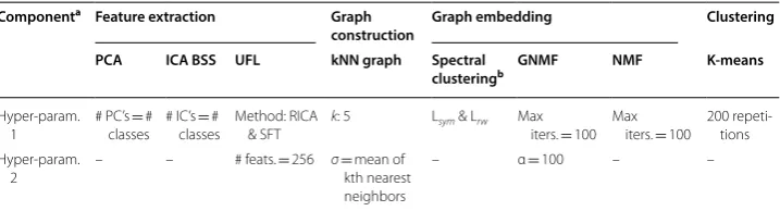
As addressed in Dizaji et al. [14], successful clustering algorithms need to have a few hyper-parameters for wide applicability in real-world situations. Dizaji et al. [14] in their deep learning-based clustering algorithm, limited their hyper-parameter space to a fixed set of values, i.e., they did not perform a parameter search. Following the same principle, the hyper-parameter values used in our clustering processing are summarized in Table 2.
In summary, the clustering methods used to achieve the aims of this study are
• Without graph embedding: K-means, PCA with K-means, and NMF with K-means.
• With graph embedding: SPC-SYM, SPC-RW, ICA-SYM, and GNMF—all of which used K-means as a final step to obtain the clusters.
The clustering experiments were implemented in the academic and industry standard numerical computing environment MATLAB (version 2017b) on a Linux based operat-ing system of Ubuntu (version 14.04). The computational environment was setup on a computer with 20 GB of memory and AMD-FX-6300 3.5 GHz 6-Core CPU.
Performance evaluation
To evaluate the clusters, the standard protocol and performance metrics provided in other studies [8, 14, 52] are used. The number of clusters in all algorithms is provided by the number of unique ground-truth labels in each dataset. The first metric used to assess clustering performance is the normalized mutual information (NMI), which measures the dependence of two labels of the same data [53]. NMI is independent of the label permutations of the clusters and its values range from 0 (completely independent) and 1 (completely identical). The second measure, unsupervised clustering accuracy (ACC), is the common accuracy metric computed for the best matching permutation between
Table 2 Cluster processing pipeline parameters used in experiments
PC: principal component. IC: independent component. PCA: The number of features is set to the number of classes. ICA BSS: The number of source signals is set to the number of classes. UFL: The number of features is 256 for both RICA and SFT, which was determined by the source code examples from [27, 28]. kNN graph: The nearest neighbor value k is set to 5, as in Cai et al. [7]. The σ scaling factor is set to the mean of value of all of the kth nearest neighbors from the similarity matrix [19]. On large datasets, a smaller set of observations from the data is used to calculate σ, using the method of estimating population proportions [51]. Spectral Clustering: Two types of normalized graph Laplacians were used, the symmetric Laplacian and random walk Laplacian [19]. GNMF and NMF: The default parameters as provided in the code available from Cai et al. [7] were used. K-means algorithm: 200 repetitions of the algorithm were used in order to obtain stable clusters a Some processing components have more than one hyper-parameter. Thus, a second hyper-parameter is provided where needed
b Spectral clustering also refers to the use of eigendecomposition for the Laplacian matrix
Componenta Feature extraction Graph
construction Graph embedding Clustering PCA ICA BSS UFL kNN graph Spectral
clusteringb GNMF NMF K‑means
Hyper-param. 1
# PC’s = # classes
# IC’s = # classes
Method: RICA & SFT
k: 5 Lsym & Lrw Max iters. = 100
Max iters. = 100
200 repeti-tions Hyper-param.
2
– – # feats. = 256 σ= mean of kth nearest neighbors
clustered labels and ground-truth labels, provided by the Hungarian algorithm [54]. Implementation details about the two metrics can be found in Xu et al. [53]. Calculating the ACC and NMI allows the results obtained in this study to be compared with almost any other clustering study, since these two metrics are the most widely used for evalua-tion. This is evidenced especially in the most recent state-of-the-art clustering methods [14, 23].
Results
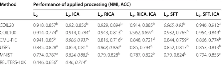
The results of implementing the new clustering pipeline on the six datasets are provided here. Performing ICA blind source separation, after the initial matrix factorization step, provided the maximum clustering performance (Table 3) in four out of six datasets (COIL100, CMU-PIE, MNIST, and REUTERS-10K). Applying UFL as an initial process-ing component helped to provide the maximum performance in three out of six data-sets (USPS, COIL20, and COIL100). Although on the COIL100 dataset, where both ICA BSS and UFL increased performance, no interaction effect between the two processing components has been shown (see the multivariate analysis of variance provided below). Furthermore, across all datasets the maximum performing clustering algorithms were GNMF (COIL100 and USPS), SPC-SYM, (COIL20 and MNIST) and PCA (CMU-PIE and REUTERS-10K) as shown in Table 3. This demonstrates that in four out of six data-sets, graph-based clustering provides the maximum performance. None of the datasets exhibited maximum performance without using ICA BSS and/or UFL, which demon-strates that at least one type of the processing components is necessary to achieve the best clustering.
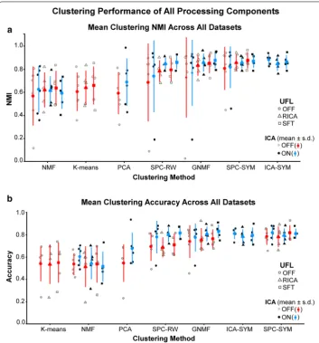
To test the statistical significance and any interaction of the processing components, a three-way multivariate analysis of variance (MANOVA) was performed. The MANOVA revealed that there is no significant interaction among ICA BSS, unsupervised feature learning, and clustering methods (Pillais’ Trace = 0.009, F(6,166) = 0.0959, p < n.s.). This demonstrates that the performance effects of the three components are independent of each other (as shown by the NMI results in Fig. 2a and ACC results in Fig. 2b).
The key results of the processing components on each of the six datasets are summa-rized below:
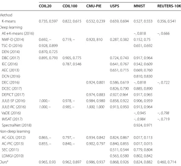
Table 3 Comparison of maximum performance across processing components
Both NMI and ACC are presented in each cell, where the first value is the NMI. Italic font within a row indicates the maximum performance obtained for a dataset. The clustering algorithm providing the maximum performance for a given processing component and dataset is indicated by the following symbols: aGNMF; bSPC-SYM; cPCA; dSPC-RW; eICA-SYM
Method Performance of applied processing (NMI, ACC)
L2 L2, ICA L2, RICA L2, RICA, ICA L2, SFT L2, SFT, ICA
COIL20 0.918, 0.857b 0.92, 0.856b 0.929, 0.894b 0.914, 0.885b 0.965, 0.93b 0.946, 0.912a
COIL100 0.914, 0.774b 0.914, 0.784a 0.943, 0.813b 0.962, 0.897a 0.932, 0.765b 0.954, 0.849a
CMU-PIE 0.941, 0.85b 0.986, 0.937c 0.816, 0.716b 0.848, 0.721d 0.844, 0.759b 0.866, 0.774b
USPS 0.845, 0.828a 0.854, 0.81a 0.868, 0.926a 0.85, 0.794e 0.852, 0.817b 0.853, 0.813b
MNIST 0.774, 0.787a 0.824, 0.882b 0.79, 0.828b 0.787, 0.822b 0.79, 0.824b 0.794, 0.853a
• COIL20: Feature learning using SFT with SPC-SYM provided the highest clus-tering performance (NMI = 0.965, ACC = 0.93), which is better than the baseline SPC-SYM clustering performance (NMI = 0.918, ACC = 0.857). With SFT and ICA BSS, GNMF also showed an improvement in both performance measures
Fig. 2 Mean clustering performance. The mean performances (with ± s.d. error bars) are laid on top of the individual cluster performances. The clustering methods are organized in ascending order for each performance measure. Under the UFL legend, “OFF” indicates that only L2-normalized features were used for
clustering. This means that no feature extraction was performed. a Mean NMI across all datasets. b Mean ACC across all datasets. The MANOVA revealed that there was a statistically significant difference in applying ICA BSS after the matrix factorizations (Pillais’ Trace = 0.058, F(1,166) = 4.05, p < 0.05). The post hoc pairwise t-tests show that ICA BSS provides higher mean performance across all datasets (NMI: µICA-ON= 0.783 ± 0.174 and
µICA-OFF= 0.716 ± 0.20, p < 0.05; ACC: µICA-ON= 0.745 ± 0.133 and µICA-OFF= 0.653 ± 0.165, p < 0.001). MANOVA
also showed there was significant difference in clustering method (Pillais’ Trace = 0.54, F(6,166) = 8.14,
p < 0.001). GNMF, SPC-RW, SPC-SYM, and ICA-SYM had the higher mean performance compared to all other clustering methods (all comparisons p < 0.001), but there was no statistical difference among these four methods. The UFL processing component was significant at the less stringent p= 0.1 level (Pillais’ Trace = 0.063, F(2,166) = 2.14, p < 0.1). Post-hoc pairwise t-tests at the p < 0.05 level show that the NMI performance is higher with RICA (µUFL-RICA= 0.774 ± 0.137) and SFT (µUFL-SFT= 0.786 ± 0.144) feature learning
in comparison to the absence of feature learning (µUFL-OFF= 0.706 ± 0.238). All post hoc pairwise t-tests were
(NMI = 0.946, ACC = 0.912) compared to its baseline GNMF clustering perfor-mance (NMI = 0.913, ACC = 0.844).
• COIL100: The best clustering performance (NMI = 0.962, ACC = 0.897) was obtained with GNMF clustering using RICA feature learning and ICA BSS. Without feature learning and ICA BSS, GNMF performance is (NMI = 0.9, ACC = 0.713). The addition of the RICA feature learning increases the per-formance to (NMI = 0.926, ACC = 0.74). The application of ICA BSS to GNMF using only L2-normalized features increases the clustering performance to (NMI = 0.914, ACC = 0.784).
• CMU-PIE: Clustering performance obtained with SPC-SYM and ICA BSS is (NMI = 0.947, ACC = 0.879), which is an improvement over the baseline SPC-SYM implementation (NMI = 0.941, ACC = 0.85). However, when the simpler method of clustering on the PCA reduced representation of the pixels, followed by ICA BSS, K-means clustering provides the top performance (NMI = 0.985, ACC = 0.937). Without any ICA BSS, clustering in the PCA representation provides only (NMI = 0.534, ACC = 0.231) performance. The best clustering performance using feature learning was obtained with SFT combined with ICA BSS using SPC-SYM (NMI = 0.866, ACC = 0.774), which is still lower than baseline SPC-SYM perfor-mance.
• USPS: The best clustering performance was obtained with RICA feature learning and GNMF (NMI = 0.868, ACC = 0.926). The baseline GNMF performance was (NMI = 0.854, ACC = 0.828), which was higher than the baseline SPC-SYM per-formance (NMI = 0.842, ACC = 0.814). When the ICA BSS was applied to GNMF, the performance of the NMI increased, but the accuracy decreased (NMI = 0.854, ACC = 0.810).
• MNIST: The best clustering performance was obtained with SPC-SYM/SPC-RW using ICA BSS (NMI = 0.824, ACC = 0.882). The performance of the base-line SPC-SYM and SPC-RW were (NMI = 0.779, ACC = 0.756) and (NMI = 0.757, ACC = 0.67), respectively. When RICA feature learning was applied to SPC-SYM, the performance increased to (NMI = 0.79, ACC = 0.828). When ICA BSS was com-bined with RICA feature learning for SPC-SYM, the performance decreased slightly (NMI = 0.787, ACC = 0.822). With GNMF clustering, the baseline performance (NMI = 0.774, ACC = 0.787) improved when ICA source was applied (NMI = 0.813, ACC = 0.845). Improvement to the GNMF baseline performance was also achieved when SFT feature learning was combined with ICA BSS (NMI = 0.794, ACC = 0.853).
• REUTERS-10K: When PCA dimension reduction followed by ICA BSS is applied directly applied to the tf-idf matrix, K-means clustering provides the top clustering performance (NMI = 0.46, ACC = 0.714). Without ICA BSS, PCA dimension reduc-tion provides an accuracy of (NMI = 0.446, ACC = 0.656). The next best clustering performance was provided by NMF without (NMI = 0.318, ACC = 0.546) and with ICA BSS (NMI = 0.428, ACC = 0.638).
outperformed all other state-of-the-art non-deep learning clustering methods (Table 4). With respect to deep learning-based clustering algorithms, our methodology performed second best after the JULE algorithms (JULE-SF and JULE-RC) in three out of six data-sets (COIL20, COIL100, and CMU-PIE).
The main comparison results from Table 4 for each of the six datasets are summa-rized below:
• COIL20: Our SPC-SYM with SFT feature learning was 3.5 percentage points (p.p.) less than JULE (both JULE-SF and JULE-RC had perfect NMI) in NMI perfor-mance. The JULE algorithms denoted by JULE-SF and JULE-RC, are the same
Table 4 Comparison of clustering performance across different datasets and clustering techniques
a The maximum clustering performance obtained by the processing components proposed in this study is provided for each dataset. When available, both NMI and ACC are presented in each cell, where the first value is the NMI. If the cell is blank then the clustering method was not used on the dataset. Italic font within a row indicates the maximum performance obtained for a dataset. The full names and references of the compared methods are: Deep Embedding Network (DEN) [11], Discriminatively Boosted Clustering (DBC) [55], Infinite Ensemble Clustering (IEC) [56], Autoencoder-based Clustering (AEC) [10], Deep Embedded Clustering (DEC) [8], Deep Clustering Network (DCN) [13], Deep Convolutional Embedded Clustering (DCEC) [57], Deep Embedded Regularized Clustering (DEPICT) [14], Variational Deep Embedding (VaDE) [15], autoencoder with K-means clustering (AE + K-means) [8], Information Maximizing Self-Augmented Training (IMSAT) [58], NMF with Deep learning model (NMF-D) [59], Joint Unsupervised Learning (JULE) “-SF” and “-RC” [16], Task-specific Deep Architecture for Clustering (TSC-D) [60] Graph Degree Linkage-based Agglomerative Clustering (AC-GDL) [61] and Agglomerative Clustering via Path Integral (AC-PIC) [62], Spectral Embedded Clustering (SEC) [63], and Local Discriminant Models and Global Integration (LDMGI) [52]
Baseline Performance of applied processing on different datasets (NMI, ACC)
COIL20 COIL100 CMU‑PIE USPS MNIST REUTERS‑10K
Method
K-means 0.735, 0.597 0.822, 0.615 0.532, 0.239 0.659, 0.694 0.527, 0.553 0.356, 0.541 Deep learning
AE+K-means (2016) –, 0.818 –, 0.666 NMF-D (2014) 0.692, – 0.719, – 0.920, 810 0.287, 0.382 0.152, 0.75
TSC-D (2016) 0.928, 0.899 0.651, 0.692 DEN (2014) 0.870, 0.725
DBC (2017) 0.895, 0.793 0.905, 0.775 0.724, 0.743 0.917, 0.964 IEC (2016) 0.787, 0.546 0.641, 0.767 0.542, 0.609 AEC (2013) 0.651, 0.715 0.669, 0.760 DCN (2016) 0.810, 0.830 DEC (2016) 0.924, 0.801 0.586, 0.619 –, 0.818 –, 0.722 DCEC (2017) 0.826, 0.790 0.885, 0.890 DEPICT (2017) 0.974, 0.883 0.927, 0.964 0.917, 0.965 JULE-SF (2016) 1.000,– 0.978, – 0.984, 0.980 0.858, 0.922 0.906, 0.959 JULE-RC (2016) 1.000, – 0.985, – 1.000, 1.000 0.913, 0.950 0.913, 0.964 VaDE (2016) –, 0.945 –, 0.798
IMSAT (2017) –, 0.984 –, 0.719 SpectralNet (2018) 0.924, 0.971
Non-deep learning
AC-GDL (2012) 0.865, – 0.797, – 0.934, 0.842 0.824, 0.867 0.017, 0.113 AC-PIC (2013) 0.855, – 0.840, – 0.902, 0.797 0.840, 0.855 0.017, 0.015 SEC (2011) 0.511, 0.544 0.779, 0.804 LDMGI (2010) 0.563, 0.580 0.802, 0.842
method except that the “–RC” is the fine-tuned version of the “straight-forward” “-SF” version [16]. Overall, SPC-SYM with SFT ranked 2nd (out of 6) compared to 5 other deep clustering methods.
• COIL100: GNMF with RICA feat learning and ICA BSS performed 1.6 p.p. and 2.3 p.p. less than JULE-SF and JULE-RC, respectively, in NMI. GNMF with RICA and ICA BSS ranked 2nd (out of 5) compared to 4 other deep clustering methods.
• CMU-PIE: The simple combination of PCA with ICA BSS performed almost on par with the much more complex JULE algorithm, which uses a combination of recur-rent and convolutional neural networks. Specifically, before any model fine-tuning is applied to the JULE algorithm (JULE-SF), our PCA and ICA combination was 0.2 p.p. higher in NMI performance. However, this advantage is lost once the JULE algo-rithm is fine-tuned (JULE-RC). PCA with ICA BSS ranked 2nd (out of 5) compared to 4 other deep cluster methods.
• USPS: Using RICA with GNMF performed third best after the JULE-RC and DEPICT algorithms, outperforming seven deep learning clustering methods. This new combination even outperformed JULE-SF by 1 p.p. in NMI and 0.4 p.p. in ACC. Overall, RICA with GNMF ranked 3rd (out of 9) compared to 8 other deep cluster-ing methods.
• MNIST: Our clustering algorithm performed better than seven other deep learning clustering algorithms by simply using ICA BSS after eigenvector decomposition of the normalized Laplacian used in SPC-SYM. However, it ranked 8th (out of 15) com-pared to 14 other deep clustering methods. Nonetheless, it performed better than the popular algorithms of DEC by 0.8 p.p. in NMI and 3.8 p.p. in ACC and DCN by 1.4 p.p. in NMI and 5.2 p.p in ACC.
• REUTERS-10K: Our implementation of clustering in the PCA space with ICA BSS, performed better than AE+K-means by 4.8 p.p. in NMI, however it did not exceed any other deep learning clustering algorithms, ranking 4th (out of 5) in comparison to 4 other deep learning methods. Nonetheless, our PCA and ICA combination per-formed on par with the DEC and IMSAT algorithms, which were 0.5 and 0.8 p.p. in NMI, respectively, better than our clustering performance.
Discussion
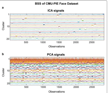
It is demonstrated that standard clustering techniques, especially graph-based methods, can be used to achieve equivalent or better clustering performance than deep learning clustering algorithms when ICA blind source separation and unsupervised feature learn-ing algorithms are applied. ICA BSS applied to either the PCA features vectors or to the graph-embedding vectors increased the saliency of the class-specific feature embedding. This is the first study to apply ICA BSS as an improvement to the multiclass problem in graph-based clustering algorithms. UFL using RICA and SFT helped build an improved similarity graph representation of the original input data, which is critical in graph-based clustering algorithms such as spectral clustering and GNMF.
In Fig. 3a, ICA BSS separates the CMU-PIE face signals into distinct sources, which are indicated by a step function-like feature in each signal. Whereas the PCA signals (Fig. 3b) do not exhibit any distinct feature across the different class source signals. With PCA, the majority of the source signal information is carried in the first few com-ponents, thus confusing the different class information. Surprisingly, in the CMU-PIE dataset, PCA with ICA BSS and K-means clustering performed better than the more advanced graph-based clustering algorithms that used UFL extracted features. This may be due to the fact that UFL may be extracting noisy features thus decreasing the
similarity graph’s representation efficacy. This may be the case when UFL feature extrac-tion has the undesired effect of decreasing baseline clustering performance for any of the clustering algorithms.
Furthermore, limiting the number principal components to only the number of classes in K-means combined with PCA, helped to extract only the pertinent class-specific fea-tures. First, PCA captures only the necessary variance by eliminating the extra informa-tion, and then BSS using ICA separates the signals pertaining to each class. Although unexpected, clustering success in the REUTERS-10K text document dataset is not alto-gether surprising. Since, ICA has been shown to perform reasonably well on text docu-ments in the task of topic classification and information retrieval [64–66].
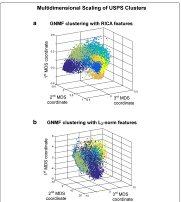
Figure 4 plots the estimated clusters obtained from GNMF for the USPS dataset using both the L2-normalized and RICA features. The L2-normalized features used for cluster-ing fail to highlight distinct groupcluster-ings (Fig. 4b) in the USPS digit data, while the RICA features provide much more compact clusters (Fig. 4a), which is also evidenced by the higher clustering NMI and ACC. This shows that employing UFL for feature extraction is better able to capture the underlying structure in data, which is important for building an accurate similarity matrix [8]. Furthermore, without any hyper-parameter search in the feature learning procedure, high clustering performance better than many advanced deep clustering techniques is achieved. In fact, by using only a consumer-level 6-core CPU (AMD-FX-6300) we are able to achieve equivalent computation times with respect to deep clustering algorithms that require high-end video cards (NVIDIA Titan X Pas-cal) [14, 16], which have many more GPU cores than standard video cards.
The limitations of the clustering methodology presented in our study are mainly due to the processing speed of the similarity graph and the matrix factorizations [23]. However, the speed limitation of the matrix factorization is due to the initial eigendecomposition and NMF computations. Otherwise, once the k basis vectors or eigenvectors have been obtained, the ICA computation is fast since the dimensionality of these vectors are small. Nonetheless, as a simple and effective boost to spectral clustering and GNMF, ICA blind source separation can be used alongside UFL with RICA or SFT.
Given the multiple stages of processing in the proposed clustering pipeline, guidelines for its recommended usage are provided. Initially, PCA with the number components set to the number of classes and ICA BSS using K-means should be applied as a sim-ple baseline. This should be an effective baseline for text documents. In image datasets, another effective baseline would be to use GNMF or SPC-SYM using ICA BSS. GNMF or SPC-SYM using UFL with RICA and SFT for feature extraction can also be used as alternate clustering algorithm. Finally, GNMF or SPC-SYM using ICA BSS and UFL fea-ture extraction can be used as a last attempt to obtain high clustering performance.
The proposed pipeline is effective for small (1000–2000 observations, such as COIL20, COIL100 and CMU-PIE) to medium-large datasets (10,000–50,000 observations, such as USPS and REUTERS10-K). Beyond 50,000 observations, deep clustering methods may be more suitable due to computation time of the similarity graphs, basis vectors, and eigenvectors [23]. The pipeline can be very useful for medical data, specifically in the analysis of electronic health records, where the number of observed patients is typi-cally ~ 1000 [67], due to the difficulty of collecting pertinent patient data. On a dataset with less than 50,000 observations, deep clustering algorithms may require too much overhead in terms of hyper-parameter setup, without providing a large improvement in terms of clustering performance.
Conclusions
From the new cluster processing pipeline presented in this study, the three main meth-odological findings are:
• Applying unsupervised feature learning to input data using either RICA or SFT, improves clustering performance.
• Surprisingly for some cases, high clustering performance can be achieved by sim-ply performing K-means clustering on the ICA components after PCA dimension reduction on the input data. However, the number of PCA and ICA signals/compo-nents needs to be limited to the number of unique classes.
The main clustering results from the new processing pipeline compared to other clus-tering studies are:
• Compared to state-of-the-art non-deep learning clustering methods, ICA BSS and/ or UFL with graph-based clustering algorithms outperformed all other methods.
• With respect to deep learning-based clustering algorithms, our new pipeline obtained the following rankings on the six different datasets: (1) COIL20, 2nd out of 5; (2) COIL100, 2nd out of 5; (3) CMU-PIE, 2nd out of 5; (4) USPS, 3rd out of 9; (5) MNIST, 8th out of 15; and (6) REUTERS-10K, 4th out of 5.
These findings demonstrate the robustness of standard clustering methods when implemented with careful processing. Instead of developing complex deep learning clustering implementations, equivalent results can be achieved from existing standard techniques with the modifications presented herein. Furthermore, the new clustering implementation presented in this study may also be used as an empirical baseline to justify use of sophisticated deep clustering learning networks and to reduce computa-tion times. For future studies, increasing the speed of building the k nearest neighbor graph used in spectral clustering and GNMF will be investigated. Also, application of the clustering pipeline to handwritten image data in another language such as Korean [68], would help to demonstrate the generalizability of the methods provided herein.
Authors’ contributions
EG conceptualized the study, performed all experiments, and analyzed all the data. EG wrote the manuscript. MM advised on the manuscript preparation and technical knowledge. Both authors read and approved the final manuscript. Acknowledgements
Not applicable. Competing interests None.
Availability of data and materials
The dataset supporting the conclusions of this article will be available on the Mendeley Data repository. Funding
This research was supported in part by the Natural Sciences and Engineering Research Council of Canada.
Publisher’s Note
Springer Nature remains neutral with regard to jurisdictional claims in published maps and institutional affiliations.
Received: 29 April 2018 Accepted: 5 August 2018
References
2. Deng J, Dong W, Socher R, Li LJ, Li K, Fei-Fei L (2009) ImageNet: a large-scale hierarchical image database. In: 2009 IEEE Conference on Computer Vision and Pattern Recognition, pp 248–255. https ://doi.org/10.1109/cvpr.2009.52068 48
3. Russakovsky O, Deng J, Su H, Krause J, Satheesh S, Ma S, Huang Z, Karpathy A, Khosla A, Bernstein M (2015) Imagenet large scale visual recognition challenge. Int J Comput Vis 115:211–252. https ://doi.org/10.1007/s1126 3-015-0816-y
4. Friedman J, Hastie T, Tibshirani R (2008) The Elements of statistical learning. Springer, New York. https ://doi. org/10.1007/b9460 8
5. MacQueen J (1967) Some methods for classification and analysis of multivariate observations. In: Proceedings of the fifth Berkeley symposium on mathematical statistics and probability, Oakland, CA, USA, pp 281–297
6. Bishop CM (2006) Pattern recognition and machine learning. Springer, New York
7. Cai D, He X, Han J, Huang TS (2011) Graph regularized nonnegative matrix factorization for data representation. IEEE Trans Pattern Anal Mach Intell 33:1548–1560. https ://doi.org/10.1109/tpami .2010.231
8. Xie J, Girshick R, Farhadi A (2016) Unsupervised deep embedding for clustering analysis. In: International Conference on Machine Learning, pp 478–487
9. Hinton GE, Salakhutdinov RR (2006) Reducing the dimensionality of data with neural networks. Science 313:504– 507. https ://doi.org/10.1126/scien ce.11276 47
10. Song C, Liu F, Huang Y, Wang L, Tan T (2013) Auto-encoder based data clustering. In: Iberoamerican Congress on Pattern Recognition, Springer, pp 117–124. https ://doi.org/10.1007/978-3-642-41822 -8_15
11. Huang P, Huang Y, Wang W, Wang L (2014) Deep embedding network for clustering. In: Pattern Recognition (ICPR), 2014 22nd International Conference on, IEEE, pp 1532–1537. https ://doi.org/10.1109/icpr.2014.272
12. Vincent P, Larochelle H, Lajoie I, Bengio Y, Manzagol P-A (2010) Stacked denoising autoencoders: learning useful representations in a deep network with a local denoising criterion. J Mach Learn Res 11:3371–3408
13. Yang B, Fu X, Sidiropoulos ND, Hong M (2017) Towards K-means-friendly spaces: simultaneous deep learning and clustering. In: Precup D, Teh YW (eds) Proceedings of the 34th International Conference on Machine Learning, PMLR, International Convention Centre, Sydney, Australia, pp 3861–3870
14. Dizaji KG, Herandi A, Deng C, Cai W, Huang H (2017) Deep clustering via joint convolutional autoencoder embed-ding and relative entropy minimization. In: 2017 IEEE International Conference on Computer Vision (ICCV), IEEE, pp 5747–5756. https ://doi.org/10.1109/iccv.2017.612
15. Jiang Z, Zheng Y, Tan H, Tang B, Zhou H (2016) Variational deep embedding: An unsupervised and generative approach to clustering. ArXiv Prepr. ArXiv161105148
16. Yang J, Parikh D, Batra D (2016) Joint unsupervised learning of deep representations and image clusters. In: Proceed-ings of the IEEE Conference on Computer Vision and Pattern Recognition, pp 5147–5156. https ://doi.org/10.1109/ cvpr.2016.556
17. Shi J, Malik J (2000) Normalized cuts and image segmentation. IEEE Trans Pattern Anal Mach Intell 22:888–905. https ://doi.org/10.1109/34.86868 8
18. Ng AY, Jordan MI, Weiss Y (2002) On spectral clustering: analysis and an algorithm. In: Advances in neural informa-tion processing systems, pp 849–856
19. Von Luxburg U (2007) A tutorial on spectral clustering. Stat Comput 17:395–416
20. Zhang Z, Jordan MI (2008) Multiway spectral clustering: a margin-based perspective. Stat Sci 23:383–403 21. Stella XY, Shi J (2003) Multiclass spectral clustering. In: Proceedings Ninth IEEE International Conference on
Com-puter Vision. IEEE, pp 313–319. https ://doi.org/10.1109/iccv.2003.12383 61
22. Tian F, Gao B, Cui Q, Chen E, Liu T-Y (2014) Learning deep representations for graph clustering. In: AAAI, pp 1293–1299
23. Shaham U, Stanton K, Li H, Nadler B, Basri R, Kluger Y (2018) SpectralNet: spectral clustering using deep neural networks. ArXiv Prepr. ArXiv180101587
24. Coates A, Ng A, Lee H (2011) An analysis of single-layer networks in unsupervised feature learning. In: Proceedings of the fourteenth international conference on artificial intelligence and statistics, pp 215–223
25. Chan T-H, Jia K, Gao S, Lu J, Zeng Z, Ma Y (2015) PCANet: a simple deep learning baseline for image classification? IEEE Trans Image Process 24:5017–5032. https ://doi.org/10.1109/TIP.2015.24756 25
26. Hyavrinen A, Karhunen J, Oja E (2001) Independent component analysis. Wiley, New York. https ://doi. org/10.1002/04712 21317
27. Le QV, Karpenko A, Ngiam J, Ng AY (2011) ICA with reconstruction cost for efficient overcomplete feature learning. In: Advances in neural information processing systems, pp 1017–1025
28. Ngiam J, Chen Z, Bhaskar SA, Koh PW, Ng AY (2011) Sparse filtering. In: Advances in neural information processing systems, pp 1125–1133
29. Nene SA, Nayar SK, Murase H (1996) Columbia object image library (coil-20)
30. Sim T, Baker S, Bsat M (2002) The CMU pose, illumination, and expression (PIE) database, IEEE, pp 53–58. https ://doi. org/10.1109/afgr.2002.10041 30
31. Matlab Codes and Datasets for Subspace Learning and Dimensionality Reduction. http://www.cad.zju.edu.cn/ home/dengc ai/Data/MLDat a.html. Accessed 12 Apr 2018
32. LeCun Y (1998) The MNIST database of handwritten digits. http://yann.lecun .com/exdb/mnist . Accessed 15 Septem-ber 2017
33. Leskovec J, Rajaraman A, Ullman JD (2014) Mining of massive datasets. Cambridge University Press, Cambridge. https ://doi.org/10.1017/CBO97 81139 92480 1
34. Oja E (1992) Principal components, minor components, and linear neural networks. Neural Netw 5:927–935 35. Deerwester S, Dumais ST, Furnas GW, Landauer TK, Harshman R (1990) Indexing by latent semantic analysis. J Am
Soc Inf Sci 41:391
37. Gultepe E, Conturo TE, Makrehchi M (2018) Predicting and grouping digitized paintings by style using unsupervised feature learning. J Cult Herit 31:13–23. https ://doi.org/10.1016/j.culhe r.2017.11.008
38. Choi S, Cichocki A, Park H-M, Lee S-Y (2005) Blind source separation and independent component analysis: a review. Neural Inf Process Lett Rev 6:1–57
39. Belouchrani A, Abed-Meraim K, Cardoso J-F, Moulines E (1997) A blind source separation technique using second-order statistics. IEEE Trans Signal Process 45:434–444
40. Delorme A, Makeig S (2004) EEGLAB: an open source toolbox for analysis of single-trial EEG dynamics including independent component analysis. J Neurosci Methods 134:9–21
41. Vigário RN (1997) Extraction of ocular artefacts from EEG using independent component analysis. Electroencepha-logr Clin Neurophysiol 103:395–404
42. Calhoun VD, Adali T, Pearlson GD, Pekar J (2001) A method for making group inferences from functional MRI data using independent component analysis. Hum Brain Mapp 14:140–151
43. McKeown MJ, Sejnowski TJ (1998) Independent component analysis of fMRI data: examining the assumptions. Hum Brain Mapp 6:368–372
44. Nascimento M, e Silva FF, Sáfadi T, Nascimento ACC, Ferreira TEM, Barroso LMA, Ferreira Azevedo C, Guimarães SEF, Serão NVL (2017) Independent component analysis (ICA) based-clustering of temporal RNA-seq data. PLoS ONE 12:e0181195
45. Bartlett MS, Movellan JR, Sejnowski TJ (2002) Face recognition by independent component analysis. IEEE Trans Neural Netw Publ IEEE Neural Netw Counc 13:1450
46. Hyvärinen A, Oja E (2000) Independent component analysis: algorithms and applications. Neural Netw 13:411–430 47. Lewicki MS, Sejnowski TJ (2000) Learning overcomplete representations. Neural Comput 12:337–365
48. Coates A (2012) Demystifying unsupervised feature learning. Dissertation, Stanford University
49. Coates A, Ng AY (2012) Learning feature representations with k-means. In: Montavon G, Orr GB, Müller KR (eds) Neural networks: tricks of the trade. Springer, Berlin, pp 561–580. https ://doi.org/10.1007/978-3-642-35289 -8_30 50. Lee DD, Seung HS (1999) Learning the parts of objects by non-negative matrix factorization. Nature 401:788 51. Thompson SK (2012) Sampling, 3rd edn. Wiley, Hoboken. https ://doi.org/10.1002/97811 18162 934
52. Yang Y, Xu D, Nie F, Yan S, Zhuang Y (2010) Image clustering using local discriminant models and global integration. IEEE Trans Image Process 19:2761–2773
53. Xu W, Liu X, Gong Y (2003) Document clustering based on non-negative matrix factorization. In: Proceedings of the 26th annual international ACM SIGIR conference on Research and development in informaion retrieval, ACM, pp 267–273. https ://doi.org/10.1145/86048 4.86048 5
54. Kuhn HW (1955) The Hungarian method for the assignment problem. Nav Res Logist Q 2:83–97
55. Li F, Qiao H, Zhang B, Xi X (2017) Discriminatively boosted image clustering with fully convolutional auto-encoders. ArXiv Prepr. ArXiv170307980
56. Liu H, Shao M, Li S, Fu Y (2016) Infinite ensemble for image clustering. In: Proceedings of the 22nd ACM SIGKDD International Conference on Knowledge Discovery and Data Mining, ACM, pp 1745–1754
57. Guo X, Liu X, Zhu E, Yin J (2017) Deep clustering with convolutional autoencoders. In: International Conference on Neural Information Processing, Springer, pp 373–382. https ://doi.org/10.1007/978-3-319-70096 -0_39
58. Hu W, Miyato T, Tokui S, Matsumoto E, Sugiyama M (2017) Learning discrete representations via information maxi-mizing self-augmented training. In: Precup D, Teh YW (eds) Proceedings of the 34th International Conference on Machine Learning. PMLR, International Convention Centre, Sydney, Australia, pp 1558–1567
59. Trigeorgis G, Bousmalis K, Zafeiriou S, Schuller B (2014) A deep semi-nmf model for learning hidden representations. In: International Conference on Machine Learning, pp 1692–1700
60. Wang Z, Chang S, Zhou J, Wang M, Huang TS (2016) Learning a task-specific deep architecture for clustering. In: Proceedings of the 2016 SIAM International Conference on Data Mining, SIAM, pp 369–377. https ://doi. org/10.1137/1.97816 11974 348.42
61. Zhang W, Wang X, Zhao D, Tang X (2012) Graph degree linkage: agglomerative clustering on a directed graph. In: European Conference on Computer Vision, Springer, pp 428–441. https ://doi.org/10.1007/978-3-642-33718 -5_31 62. Zhang W, Zhao D, Wang X (2013) Agglomerative clustering via maximum incremental path integral. Pattern
Recog-nit 46:3056–3065
63. Nie F, Zeng Z, Tsang IW, Xu D, Zhang C (2011) Spectral embedded clustering: a framework for in-sample and out-of-sample spectral clustering. IEEE Trans Neural Netw 22:1796–1808
64. Mirowski P, Ranzato M, LeCun Y (2010) Dynamic auto-encoders for semantic indexing. In: Proceedings of the NIPS 2010 Workshop on Deep Learning 2010, pp 1–9
65. Kolenda T, Hansen LK, Sigurdsson S (2000) Independent components in text. In: Advances in Independent Compo-nent Analysis, Springer, pp 235–256. https ://doi.org/10.1007/978-1-4471-0443-8_13
66. Chagnaa A, Ock C-Y, Lee C-B, Jaimai P (2007) Feature extraction of concepts by independent component analysis. J Inf Process Syst 3:33–37
67. Gultepe E, Green JP, Nguyen H, Adams J, Albertson T, Tagkopoulos I (2013) From vital signs to clinical outcomes for patients with sepsis: a machine learning basis for a clinical decision support system. J Am Med Inform Assoc 21:315–325. https ://doi.org/10.1136/amiaj nl-2013-00181 5