R E S E A R C H
Open Access
PreCount: a predictive model for
correcting real-time occupancy count data
Fisayo Caleb Sangogboye
*and Mikkel Baun Kjærgaard
*Correspondence: [email protected]
SDU Center for Energy Informatics Mærsk McKinney Møller Institute University of Southern Denmark, Odense, Denmark
Abstract
Sensing the number of people occupying a building in real-time facilitates a number of pervasive applications within the area of building energy optimization and adaptive control. To ascertain occupant counts, the adoption of camera-based sensors i.e. 3D stereo-vision and thermal cameras have grown significantly. However, camera-based sensors can only produce occupant counts with accumulating errors. Existing methods for correcting such errors can only correct erroneous count data at the end of the day and not in real-time. However, many applications depend on real-time corrected counts. In this paper, we present an algorithm named PreCount for accurately
correcting raw counts in real-time. The core idea of PreCount is to learn error estimates from the past. We evaluated the accuracy of the PreCount algorithm using datasets from four buildings. Also, the Normalized Root Mean Squared Error was used to evaluate the performance of PreCount. Our evaluation results show that in real-time PreCount achieved a significantly lower Normalized Root Mean Squared Error compared to raw counts and other correction approach with a maximum error reduction of 68% when benchmarked with ground truth data. By presenting a more accurate algorithm for estimating occupant counts in real-time, we hope to enable buildings to better serve the actual number of people to improve both occupant comfort and energy efficiency.
Keywords: Occupant count, Real-time system, Machine learning, Energy optimization
Introduction
Estimating the number of people in commercial and public buildings with the aid of pervasive sensors is receiving increasing attention. This is because the permeation of pervasive computing have prospects in facilitating several building applications. One application area customary to commercial outlets is in the area of disaster prevention and management. Most commercial outlets are mandated by government laws to provide accurate estimates of occupant counts in real-time. Lastly, occupant presence is the major driving factor for energy consumption in buildings (Chang and Hong2013; Caucheteux et al. 2013). Consequently, several approaches for simulating, monitoring and optimiz-ing energy consumption in buildoptimiz-ings includoptimiz-ing the model based approaches have become prominent and have received significant research attention (Arendt et al.2016). A similar research attention is currently given to the concept of demand response (DR) in com-mercial buildings for facilitating the control of energy demand (Kjærgaard et al.2016). DR leverages on forecasts and real-time data that comprises majorly of occupant counts to schedule DR events without impeding occupant comfort. Recently, the United States
Department of Energy (US Department of Energy2017) highlighted that, obtaining very accurate occupant counts can facilitate a 30% energy savings in buildings and it can enable building management systems to achieve occupant comfort in-line with the ASHRAE standard.
A range of sensor methods has been applied for estimating occupant counts. One line of research has studied reusing common building sensors for occupant counting. These sensors includeCO2sensors, PIR sensors, energy metering, sensors of HVAC sys-tems or WiFi access points (Christensen et al. 2014). However, these sensors are very inaccurate in their estimates. Sangogboye et al. in Sangoboye and Kjærgaard (2016) highlighted that camera-based counting technologies amongst other sensors are the state-of-art method for obtaining high quality count estimates in commercial buildings. Kjærgaard et al. (2016) corroborated this proposition by benchmarking the raw counts retrieved from both 3D stereo-vision cameras and PIR sensors with manual ground truth count estimates. The obtained count estimates from both the 3D stereo-vision cameras and PIR sensors achieved Root Mean Square Errors (RMSE) of 3.3 and 21.7, respectively.
However, while camera-based count estimates are more accurate than count estimates from other sensors, these sensor suffers from errors that are accumulated and propagated over time. For instance, when a camera sensor misses an occupant, this error is propa-gated until another offsetting error occurs or a correction approach is adopted to remove the error (Beltran et al.2013). These errors are a result of several causes such as poor lighting condition and occlusion. The state-of-art methods for correcting such erroneous count estimates are only capable of correcting erroneous counts in the past and not in real-time. This is because, these past correction methods are governed by constraints that require data until the end of the day. Subsequently, statistics about this data are used to formulate an appropriate correction model for a day (Sangoboye and Kjærgaard2016; Hutchins et al.2007; Kuutti et al.2014).
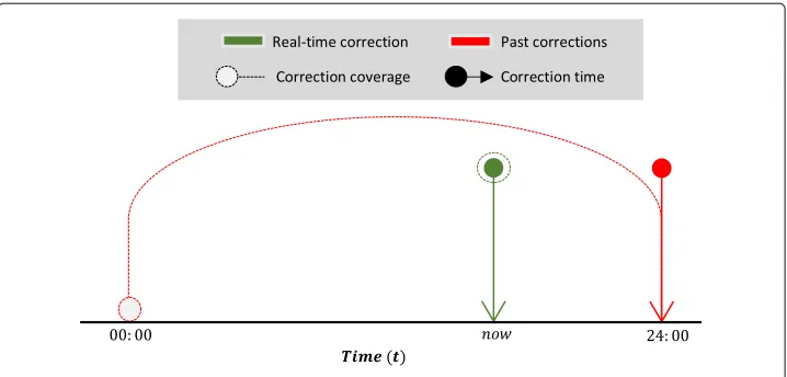
The topic of correcting erroneous count estimates in real-time is to the best of our knowledge uncharted and it differs from the previously stated approaches for correcting counts estimates in the past. Figure1illustrates the difference between past correction and real-time correction. Here, past corrections are computed at end of the day t24:00 and it covers count correction fromt24:00back to the beginning of the dayt00:00. Con-versely, real-time corrections are computed at timetnow and it only covers the current
time of the day. For instance, the past correction algorithm presented in Sangoboye and Kjærgaard (2016) cannot suffice for real-time correction because they require count data for the whole day. This count data is used to instantiate the upper bound of the probability and propagation matrices that are used in estimating count errors. Table1 cat-egorizes these past correction methods into two approaches according to their correction methodologies and inherent constraints.
Fig. 1Real-time correction versus past correction
correction, the naive approach can be easily adapted for correcting count estimates in real-time, but it does not provide high accuracy.
In this paper, we present PreCount - an algorithm for estimating count errors in real-time via a predictive model. This algorithm leverages the accuracy of the probabilistic correction methods to model erroneous counts in a dataset. Subsequently, it utilizes the derived model to accurately determine the error estimates in real-time. We make the following contributions:
1. Formulate the real-time occupant count estimation problem using past corrections and their corresponding erroneous raw counts.
2. Present the PreCount algorithm, how it trains several correction models and utilizes the best correction model to estimate count error in time.
3. Present a feature analysis and preparation process that robustly identify count errors.
4. Present an extensive evaluation result that highlights the overall performance of PreCount in four building cases. Datasets from the first three building cases were used to concretize and evaluate our design assumptions. The dataset from the last building case was used to test and validate these design assumptions. Also, we evaluate PreCount for different sizes of training data.
Table 1Approaches for past correction
Methodology Constraints
Naive approach
1. It subdivides past raw counts into daily profiles with timestamps{t0,. . .,tn}, where
nis the end of the day.
It assumes that most buildings have periods during night time where the number of occupants go to zero.
2. It initializes the first transition of each day i.e. transition at timet0to zero.
3. It assigns zero to all negative counts. Probabilistic
approach
1. It subdivides past raw counts into daily profiles with timestamps{t0,. . .,tn}, where
nis the end of the day.
1. It requires the observed maximum number of occupants to formulate and compute a transition matrix.
2. It corrects each daily profile at time tn using specific methods proposed in either Sangoboye and Kjærgaard (2016) and Kuutti et al. (2014).
The paper is structured as follows. In the “Related work” section, we present the state-of-art that highlights the methods for correcting erroneous occupant counts in the past. In the “PreCount” section, we introduce the PreCount algorithm and its elements. This “Evaluation” section includes a detailed description of the feature preparation stage and the correction methods used for correcting erroneous occupant counts in real-time. In the same section, we present the building cases and datasets used in this paper, the error patterns in our datasets and we justify the relevant features for identifying count errors in real-time. In the “Evaluation” section, we evaluate the performance of PreCount with three evaluation cases and with the datasets from the four building cases. In the “Discussion” section, we discuss the limitations of this study and propose relevant improvement opportunities. Finally, we conclude in the “Conclusions” section.
Related work
In this section, we present the State of the art for correcting and estimating occupancy count in buildings. In the first subsection, we present the state-of-art for correcting count errors in camera technologies while in the second subsection, we present other related works for estimating occupant count in buildings.
Occupant count correction methods
Ihler et al. (Ihler et al.2006) proposes a probabilistic method for correcting past raw counts obtained from a single sensor system. This method models count data from a single sensor by formulating a probabilistic model for each sensor, and the model differ-entiates between usual activity and an unusual burst of occupant count. The models are trained with six weeks of data. An inhomogeneous Poisson process is used to represent usual human activity while a hidden Markov process is used to model bursts of unusual behavior. Hutchins et al. (Hutchins et al.2007) extends this method to a multi-sensor environment by linking individual sensor streams to form a multiple-sensor probabilistic model. This multiple-sensor probabilistic model is represented using a directed graphical model and it is used for estimating occupant counts in buildings.
On the other hand, Sangogboye et al. (Sangoboye and Kjærgaard 2016) introduces
a training free probabilistic approach for correcting past counts named PLCOUN T.
PLCOUN T takes both occupant transitions and cumulative counts as input to
formu-late an occupant count problem in the form of both a probability and propagation matrix respectively. Given this formulation, PLCOUN T initializes a probability matrix by estimating the likelihood that a space is occupied by a specific number of peo-ple. Subsequently, PLCOUN T computes the remaining time steps until the end of the day in the probability matrix by estimating the probabilities of measured count transi-tions. Lastly, PLCOUN T performs a backtracking operation on the propagation matrix to compute a new count estimate for each time step.PLCOUN Treported an 86% error reduction when it is compared to raw counts and benchmarked with ground truth count data.
Occupant count estimation methods
node sensor network of cameras (Kamthe et al.2009). This work proposed two models -the closed distance Markov chain and -the blended Markov chain for model occupant transitions between states. Erickson et al. evaluated the proposed models using three evaluation metrics - occupant variation, Jensen Shannon divergence and occupant arrival and departure rates. The obtained evaluation result indicates that both the blended Markov chain model and the closest distance Markov chain achieved similar performance with the Jensen Shannon metric while the blended Markov chain model achieved better performance for other metrics.
Beltran et al. proposed ThermoSense (Beltran et al. 2013) for estimating occupant counts with PIR sensors and thermal based sensing. The PIR sensor is used to determine the presence of occupants in rooms while the thermal based sensing is used to detect the thermal footprint of occupants for deriving the count of occupants in a room. The PIR sensor also helps to reduce the amount of energy used by the thermal-based sensor and other components of the sensing system. To facilitate the count of people in a room, ThermoSense firstly creates a thermal map when a room is unoccupied. This map is con-tinually updated using the lowest temperature during times when the room is occupied or every 15 min when no movement is discovered in a room. Secondly, ThermoSense con-verts a measured 8X8 grid temperature values to create three feature vectors for training and comparing three different prediction methods – Artificial Neural Network (ANN), K-Nearest Neighbor (KNN) and Linear regression. The three feature vectors include the total active points, number of connected components and size of the largest compo-nent. Subsequently, an average filter is applied to the obtained raw occupancy estimate. The comparative result obtained shows that the KNN classifier achieved the leastNRMSE value of 25%.
Erickson et al. (2009) deployed a wireless camera sensor network (Kamthe et al.2009) for facilitating the estimation of occupant mobility patterns in a large multi-function university building. This work uses two predictive models for learning and estimating occupant counts. The first model - a multivariate-gaussian method learns and predict the count estimate of an occupant in a building. While the second model - an agent-based model simulates the mobility patterns of occupants. The multivariate model partitions occupant count data from several locations in a building into hourly slots and compute the mean and standard deviate for each slot. These estimates with probability distribu-tion funcdistribu-tion and some expert assumpdistribu-tions from ground truth observadistribu-tions are used for randomly and collectively draw occupant distribution for each location. The agent-based model, on the other hand, is used to simulate each occupant’s movement by modeling itineraries, path choice, and walking behavior. The evaluation result of both models shows similar performance and indicates that the multivariate model achieved an average NRMSEof 42.6% while the agent-based model achieved an averageNRMSEof 43.3% for
two rooms respectively.
a minimum and maximum accuracy and RMSE of 67% and 1.01 and 75% and 0.77 respectively.
Ken et al. (Christensen et al.2014) investigated three tiers of implicit occupant estima-tion that reuses existing infrastructure in buildings. The first tier involves the sole use of existing infrastructure such as Dynamic Host Control Protocol (DHCP) and Address Resolution Protocol (ARP) of network infrastructures to determine occupant counts. The second tier involves the augmentation of existing building infrastructure with an additional software component. For example, the Simple Network Management Proto-col (SNMP) can be used to extract occupant activities such as typing. Also, additional software can be installed on host devices to obtain occupant location by laterating the signal strength of multiple Access points (AP). The third tier involves both the addition of dedicated sensors and software to existing building infrastructure. Ken et al. compared the accuracies of two implicit sensing - PC activity and DHCP with occupant estimates from PIR sensors to estimate occupant vacancy and presence. Overall, the PIR sensor, PC activity, and DHCP achieved a 91, 89 and 59% accuracy respectively.
PreCount
In this section, we propose the PreCount algorithm for accurately correcting raw counts in real-time. One approach to achieving real-time error correction from raw counts is to continuously learn the patterns and trends of count errors using machine learning approaches. We introduce the following definitions and notations to distinguish the types of datasets used in this work:
Transitions (C) represents the difference between the entries and exits for each time-step in a dataset.
Occupant Count (CC) is the cumulative sum ofCfrom the first time-step of a given day to the last time-step of that day.
We differentiateCandCCfor raw counts in the past, raw count corrections in the past and raw counts in real-time with subscriptsr,pandrtrespectively. Hence, we compute the errors of the transitions and occupant counts in our past datasets as follows:
Ce=Cp−Cr (1)
CCe=CCp−CCr (2)
PreCount employs a supervised machine learning approach to correct counts in real-time with the assumption thatCCeand error rates are repeatable over time. We validate
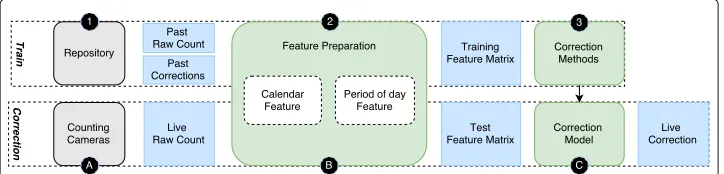
this assumption in later subsections. To achieve this aim, PreCount applies a number of steps that are highlighted in Fig.2, and we refer to the elements in the figure using their respective numbers. The rounded rectangles in the figure are the elements applied to the presented datasets, and the squared rectangles represent data. PreCount is comprised of both a training and a correction phase, and it assumes that counting cameras are avail-able to provide real-time count data(CCrt)for the correction phase. In the training phase,
PreCount assumes that a training dataset comprising of bothCCr and their
Fig. 2Overview of the PreCount algorithm
correction method introduced in Sangoboye and Kjærgaard (2016) is used to generate
CCpdataset, and it is subsequently used to computeCCeas specified in Eq.2(1).
Subse-quently, the feature preparation stage transforms the calendar and weather datasets into feature sets. This transformation is done alongside theCCr dataset and theCCedataset
to formulate a training feature matrix (2). We provide a definition and justification of the calendar and weather feature sets in later subsections. After the feature preparation stage, PreCount deploys a number of regression algorithms for correctingCCrt. These
regres-sion algorithms are trained and evaluated with the training feature matrix from the feature preparation stage, and the best performing regression model is adopted as the correction model (3). In the correction phase, PreCount retrievesCCrt from the installed
count-ing cameras (A) and it applies the same feature preparation step in the traincount-ing phase to obtain the test feature matrix (B). The selected correction model derived from (3) is used to estimate the inherent count errors inCCrt. Lastly, we use the resulting error estimates
to correctCCrt(C).
In the following subsections, we present the details of the individual elements in the proposed algorithm. Here, we proceed with a particular focus on the feature prepara-tion stage and the descripprepara-tion of the regression algorithms deployed in PreCount. In subsequent subsections, we firstly introduce the datasets used in this work. Secondly, we provide the justification for employing a machine learning approach to correct count errors in real-time. Lastly, we highlight the rationale for including both the calendar and weather features to formulate a feature matrix.
Feature preparation
The feature preparation stage entails the representation of all features sets analyzed in the feature analysis stage alongsideCCr,CC, andCCrt. This representation is used to obtain
a feature matrix comprising of both an input feature sets and a target feature sets. The feature matrix is formulated as a multi-label and multi-output problem where each label in the input feature set and the target feature set can assume a real value.
The feature preparation stage assumes that all count datasets i.e. the CCr, CC, and
the CCrt datasets have the same temporal resolution. Given that this requirement is
met, these datasets are subdivided into daily profilesdjsuch that they are comprised of
{d0,. . .,dm}days and each daydjis comprised of time slots{s0,. . .,sn}. Given this
formu-lation, theCCr,CCeand theCCrtdatasets are transformed into matrices with axes(d,s).
Algorithm 1PreCount Feature Preparation
Input: Cumulative count datasetCCrandCCporCCrt
Output: Feature matrix
1: Determine calendar features forCCrorCCrt
2: Obtain all daily profiledjinCCrorCCrtand features
3: day namednj=
⎧ ⎪ ⎪ ⎪ ⎪ ⎪ ⎨ ⎪ ⎪ ⎪ ⎪ ⎪ ⎩
0, ifdj==Sunday
1, ifdj==Monday
. . .,
6, ifdj==Saturday
4: day typedtj=
⎧ ⎨ ⎩
0, ifdj==Weekday
1, ifdj==Weekend
5: holidayhj=
⎧ ⎨ ⎩
0, ifdj==Holiday
1, ifdj==Nonholiday
6: seasonswej=
⎧ ⎪ ⎪ ⎪ ⎪ ⎪ ⎨ ⎪ ⎪ ⎪ ⎪ ⎪ ⎩
0, ifdj==Winter
1, ifdj==Spring
2, ifdj==Summer
3, ifdj==Autumn
7: Determine period-of-day features forCCrorCCrt
8: Obtain the timeslotsstin eachdjand feature
9: period-of-daypd(dj,st)= ⎧ ⎪ ⎪ ⎪ ⎪ ⎪ ⎪ ⎪ ⎪ ⎨ ⎪ ⎪ ⎪ ⎪ ⎪ ⎪ ⎪ ⎪ ⎩
0, ifst==Dawn
1, ifst==Sunrise
2, ifst==Noon
3, ifst==Sunset
4, ifst==Night
10: Formulate feature matrix
11: Determine the current time slotsk
12: ifTraining phasethen
13: Determine count errorCCe=CCp−CCr
14: Derive input feature set={dnj,dtj,hj,wej}∪{pd(dj,s0),. . .,pd(dj,sk)}∪
15: {CCrdj,s0,. . .,CCrdj,sk}
16: else ifCorrection Phasethen
17: CCe=unknown
18: Derive input feature set={dnj,dtj,hj,wej}∪{pd(dj,s0),. . .,pd(dj,sk)}∪
19: {CCrtdj,s0,. . .,CCrtdj,sk}
20: end if
21: Derive target feature set={CCedj,s0,. . .,CCedj,sk}
22: Return feature matrix={Input feature set}∪{Target feature set}
Input feature set
The input feature set of the feature matrix is comprised of the calendar feature, the period of feature and all the raw count data i.e.CCr in the training phase orCCrt in the
slot of the current day till the current time slot. The input feature set is formulated as follows:
1. determine the values of all calendar feature such as day name (dn) - {Sunday, Monday, Tuesday, Wednesday, Thursday, Friday, Saturday}, day type (dt) -{Weekday, Weekend}, holiday (hj) - {holiday, non-holiday} for eachdjinCCror CCrt. These features are represented as follows: {0, 1, 2, 3, 4, 5, 6 }, {0, 1} and {0, 1} respectively.
2. determine the period of day features (pd ) of each time slotdj,st
inCCrorCCrt to obtain the valuespdd0,s0,. . .,pddm,ss where eachpddj,stcan be one of these five
values {Dawn, Sunrise, Noon, Sunset and Night}. To further differentiate the period of day features according to seasons, we include the seasonal values (we) of each daydjinCCrorCCrt. We differentiate for all the seasons of the year {Winter, Spring, Summer, Autumn} and we represent these features as follows: {0, 1, 2, 3, 4} and {0, 1, 2, 3} respectively.
Given this formulation, the input feature set is comprised of all the aforementioned features and, raw count data
CCrdj,s0,. . .,CCrdj,sk
or
CCrtdj,s0,. . .,CCrtdj,sk
. Where
skis the current time slot, ands0is the time slot at the beginning of the day.
Target feature set
The target feature set in the training phase is comprised of the CCe dataset
CCedj,sk−q,. . .,CCedj,sk
where kis the current time slot andq is the number of time-steps to the past. CorrectingCCrtfromk−qtime slot tokis based on the rationale that
the occupant count at each time slot is partially dependent on the occupant counts from previous time slots (Sangogboye and Kjærgaard2017).
In this paper, we have varied the value ofq based on the temporal granularity of a dataset. The value ofq is computed as specified in Eq.3. In this equation, the param-eterhorizonis the recommended estimation look-ahead for an occupant model with a default value of 180 min as specified in Sangogboye and Kjærgaard (2017). In the correc-tion phase, the values ofCCeis unknown (?), and it is the value we seek to determine using
the selected correction model in the training phase.
q= horizon
temporal granularity(in minutes) (3)
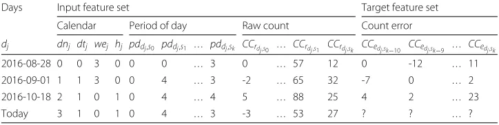
Table2presents an example feature matrix that is comprised of both an input feature set and a target feature set. In the example feature matrix, theCCrtdataset is represented in
feature vectordj = Today. The remaining prior feature vectors are the training feature
vectors.
Table 2Example of a PreCount feature matrix divided into input and target feature sets
Days Input feature set Target feature set Calendar Period of day Raw count Count error
Correction methods
In this section, we present two regression algorithms for estimating count errors inCCrt.
These regression algorithms include Random Forest (RFR) and AdaBoost Decision Tree (ADR). Both regression algorithms are trained using the derived feature matrix comprising of both the input and target feature sets. Subsequently, a regression model for predicting count errorCCeinCCrtis derived from the training process. In the following, we provide
the rationale for selecting these methods.
RFR
RFR is an ensemble method that utilizes decision trees as its primary estimators. This
ensemble method sub-samples the presented training feature matrix into equal partitions, and for each partition, it fits an estimator. Given a test sample, each of the trained models, is used to produce some target estimates. Subsequently, all target estimates are averaged to produce the final target estimate. One essential tuning parameter forRFRis the number of estimators it utilizes to fit the training feature matrix. In this paper, we have utilized ten estimators to fit the training feature matrix. This is the same number of estimators specified in Pedregosa et al. (2011a). This number of estimators is assumed to avoid over-fitting issues and to achieve model generalization.
ADR
An AdaBoost regressor is a meta-estimator (Pedregosa et al.2011b) that fits multiple instances of the same regression algorithm to a training dataset. This is achieved by first fitting a single regression method to the entire dataset, and subsequently, it fits addi-tional regression methods on the same dataset where the previous regression method are less accurate. Similar toRFR, AdaBoost ensemble enables the declaration of the num-ber of estimators to be used in the learning procedure. However, unlike theRFR where all of the declared estimators are fitted to a subset of the training dataset,ADRperforms incremental training that terminates when there is a perfect fit. Hence, the specified num-ber of estimators only provides an upper limit of the numnum-ber of estimators that can be used before the learning procedure is terminated. In this paper, we have chosen the same decision tree method as the base estimator for the AdaBoost meta-estimator hence the acronymADR. Also, we have utilized the default number of estimators of 50 presented in Pedregosa et al. (2011b) to fit the training feature matrix.
Lastly, the rationale for choosing the decision tree regression method as the base esti-mator is based on its ability to discover complex dependencies between features and its strength in modeling both linear and non-linear relationships in a feature matrix. Also given that the problem of correcting the count errorsCCein the obtained real-time count CCrtis formulated as a multi-label regression problem where each target label can assume
a real number, these correction models are utilized in this form to predict and correct the values of these labels. These labels, will enable a varying number ofCCrttuples to be
cor-rected as against the case of a single-label regression problem, where users are constrained to a single output.
Building cases and datasets
training, and evaluation. The dataset from the last building case is used to test and vali-date PreCount. The four building cases are a university teaching building (UNIVERSIT Y), a public library (LIBRARY), a shopping mall (MALL) and a research building (OFFICE). The datasets obtained from these buildings cover different ways commercial buildings
are occupied and used by people. Each dataset contains bothCandCC of both the
raw counts and their corresponding past corrections respectively. The raw count correc-tion data in the past are obtained through the probabilistic method in Sangoboye and Kjærgaard (2016).
We have obtained 1-year worth of dataset from the first three building cases and
6-month worth of dataset from the OFFICE building. The evaluation of PreCount is
done with this 1-year datasets. The evaluation uses the past correction data from the probabilistic approach as ground truth data. This is because of the cumbersome pro-cess involved in manually collecting ground truth data, especially in large commercial buildings. More so, the potency of obtaining high fidelity count estimates through the probabilistic approach provides a viable alternative for benchmarking subsequent meth-ods such as a method for correcting erroneous count estimates in real-time (Sangoboye and Kjærgaard2016). However, it should be noted that these datasets are only used for analysis, training and evaluation purposes and not for testing and validation. Additional, we have obtained 1-day of manually collected ground truth data from theOFFICE build-ing. The 6-month past count data from this building and the manually collected ground truth data are used to validate and test PreCount. In the following, we provide a detailed description of the four building cases.
The UNIVERSIT Yis an 8000m2 building that records an average of 800 to 900 occu-pants on normal weekdays. The building is primarily a teaching building with some office spaces. The types of room in this building are comprised mainly of classrooms, study zones, offices, and restrooms. To obtain the raw count of occupants in this building, 17 Stereo-vision cameras are installed to cover all transitions between all entrances and exits. The cameras installed in this building are manufactured by Xovis. All the datasets from theUNIVERSIT Yare obtained at a temporal granularity of 1 min.
TheMALLis a 36,000m2building containing 80 commercial spaces or shops. To obtain the raw counts of occupants in this building, 22 Xovis Stereo-vision cameras are installed to cover all transitions between the entrances and exits of the building. This building records an average of 4500 to 5000 occupants on weekends and 3500 to 4500 occupants on weekdays. All the datasets from theMALLare obtained at a temporal granularity of 15 min.
TheLIBRARYis a 60,000m2building that accommodates a library and business spaces. It records an average of 800 to 1000 occupants on weekdays and 400 to 600 occupants on weekends. To obtain the raw count of occupants in this building, 7 network cameras are installed to cover all transitions between the entrances and exits of the building. The cam-eras installed in this building are manufactured byAXIScommunications and are coupled with a software module namely Cognimatics TrueView People Counter to dynamically recognize people entering and exiting the building. All raw counts are publicly available in Jensen (2016), and the datasets from this building are obtained at a temporal granularity of 1 h.
university researchers. Thus it is mainly comprised of offices, laboratories, meeting rooms and restrooms. To obtain the raw count of occupants in this building, 4 Stereo-vision cam-eras are installed to cover all transitions between all entrances and exits in the building. Also, the cameras installed in this building are manufactured by Xovis. All the datasets fromOFFICEare obtained at a temporal granularity of 1 min.
Error patterns in raw occupant counts
In this section, we utilize datasets from the first three building cases to present our inves-tigation of the error pattern in raw counts. As stated earlier, if there exists a consistent and repeatable error pattern, this will provide the basis for adopting a machine learning approach to accurately estimate count errors in real-time. To investigate the assumption that an error pattern exists, we reiterate the following proposition from Ihler et al. (2006), Hutchins et al. (2007), and Sangoboye and Kjærgaard (2016).
Proposition 1The rate of count errors in counting sensors is directly proportional to the rate of transitions in the spaces they are deployed.
One imminent effect when the transition rate in a space increases is occupant occlusion. More specifically, it is well established that counting cameras generally have signifi-cant challenges in separating occupants that are occluded and this usually results in undercount errors. Sangogboye et al. (Sangoboye and Kjærgaard2016) investigated this proposition by correlatingCrandCe. The resulting correlation indicates a linear
rela-tionship betweenCrandCe. This linear relationship implies that a general increase in
Crwill usually result in an increase inCe. Similarly, in this paper, we correlate the rate
ofCr withCefor the first three building cases, and the obtained results show similar
patterns as specified in Sangoboye and Kjærgaard (2016).
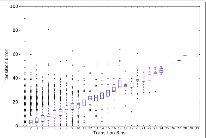
Figure3highlights the correlation results for theUNIVERSIT Ybuilding case. From this figure, it can be observed that in the x-axis, we correlated transition bins instead of the ordinaryCragainstCe. We borrowed this concept of binning from histogram charts,
and this enables us to group the sparse range of transition events in buildings. Here, we apply a bin size of 10 which implies that bin 0 contains all absolute transitions ranging from 0 to 9 while bin 1 contains all absolute transition events ranging from 10 to 19 and so on. The Pearson correlation coefficient for both variables is 0.9, and this corroborates the linear relationship observed in Sangoboye and Kjærgaard (2016).
The result from Fig.3corroborates the finding in Sangoboye and Kjærgaard (2016) that count errors follow a linear pattern. The repeatable patterns. Provide the basis for training a machine learning task.
Feature analysis
The adoption of a machine learning methodology for any given task requires the iden-tification of well-defined feature sets that can characterize both the explicit and implicit patterns within a problem domain. Within the contest of real-time error correction, such feature sets should represent the factors that influence the propagation of count errors. In the following, we present our investigation of two categories of feature sets namely the calendar and weather feature sets that influences the propagation ofCCein buildings. We
Fig. 3Correlation between transition bins (bin width = 10 counts) and absolute transition errors
regards toCCeSangoboye and Kjærgaard (2016) and Shan et al. (2003). These variabilities
were investigated by correlating count datasets with the values of these feature sets.
Calendar features
Occupant patterns in buildings vary across different types of days. Figure4highlights the occupant pattern on weekends and weekdays for theUNIVERSIT Ydataset. These patterns were derived by computing the mean of all daily profiles inCCpwith a 95% confidence
interval. Following the proposition in1, the magnitude difference in both occupant pat-terns indicates that the error rates associated with these patpat-terns will vary significantly. Also, we hypothesize that since each day of a week may be characterized by different occu-pant schedules and that more patterns may exist for other day types such as holidays, we
argue that the features set for correctingCCein real-time should include such calendar
features to navigate the different occupant patterns that may arise thereof.
Weather features
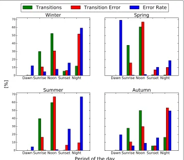
Stereo-vision, thermal and other camera technologies are significantly susceptible to poor lighting conditions (Shan et al.2003). For instance, (Shan et al.2003) indicated that this may be as a result of the predominant high luminance during summer and spring seasons, and the predominant poor luminance during autumn and winter seasons for the standard European weather condition. We utilize two independent datasets namely the period of a day and seasonal variation to investigate how the varying luminance conditions affect counting cameras.
To quantify the influence of the period of the day on count errors, we extractCpand
Cedatasets associated with the five (5) periods of the day namely:
Sunset periods between the time in the evening when the sun is about to disappear below the horizon, and the time it disappears
Noon periods between the time when the sun is at its highest point and the beginning of sunset
Sunrise periods between the time in the morning when the top of the sun breaks the horizon and the beginning of noon
Dawn periods between the time in the morning when the sun is at a specific number of degrees below the horizon and the beginning of sunrise
Night periods between the astronomical dusk of one day and the astronomical dawn of the next
The period of day dataset was obtained using a Python library given in Kennedy (2010), and these datasets are obtained at the same resolution as the count datasets and for the same coverage period.
To obtain a unified view of how both theCpandCedatasets that are associated with
each period of the day, we compute the following normalization.
ˆ
Ce(a)=
m
j=1xaj
n
i=1
m
j=1xij
(4)
wherexijdenotes thej-th element ofi-th period of the day,xajrepresents thej-th element
ofaperiod of the day andˆCe(a)is the normalized dataset ofCefor thea-th period
of the day. The value ofmmay differ depending on the number of elements inCe(a).
The same normalization is performed on theCpdataset. Subsequently, we computed
the error rate for each period of the day from the normalized datasets as follows:
ErrorRate= ˆCe
ˆ
Cp
∗100% (5)
Fig. 5Correlation between periods of the day, normalized transition and transition errors
the error rates are at the highest at dawn. Figure5also shows some distinctiveness com-pared to Fig.3. The noon period of the day has the highest proportion of all transitions for all seasons. However, the error rates during this period are low compared generally to dawn, sunset and night periods of the day. This indicates that while more accumulated Ceare propagated during periods with moreCr, the rate at which theseCeare
prop-agated are entirely independent of the rate ofCr. We argue that this variation in error
rates are well captured with the period of the day and seasonal variation feature sets.
Evaluation
at a time stamp can be zero, especially at night times and we want to avoid division by zero. TheNRMSEis derived from the root mean squared error (RMSE) as follows:
RMSE=
o
i=0
CCg(i)−CCrtc(i)
o (6)
NRMSE= RMSE CCg
(7)
where CCg(i) and CCrtc(i) are ground truth occupant counts and real-time corrected counts respectively.
For each presented building cases and their datasets, we have utilized the entire training data to benchmark the performance of the presented correction methods. Additionally, we utilized the 1-day ground truth data from OFFICE to validate PreCount’s correc-tion methods. We also present an investigacorrec-tion into correccorrec-tion cases where few datasets are available for training and we highlight how the correction results vary given these variations in the size of training datasets.
PreCount and its elements are implemented in Python using some Python data processing (Jones et al.2001) and machine learning libraries (Pedregosa et al.2011c).
In the following we present the evaluation cases used to evaluate the performance of PreCount:
1. We compare the overall performance of PreCount’s correction methods for each building case and present the most accurate correction method as PreCount. In this evaluation case, we benchmark all methods withCCpand we compare the correction methods with both theCCrtand the naive approach.
2. We compare the performance of PreCount’s correction methods in theOFFICE
building case for the 1-day ground truth data. In this evaluation case, we benchmark all the methods for correction with the ground truth data, and we compare the performance of PreCount’s correction methods with the count estimates from the naive approach,CCp, andCCrt.
3. Lastly, we evaluate the performance of PreCount with different sizes of training datasets. For this evaluation, we varied the sizes of training datasets from 30 to 120 days. This evaluation is especially crucial in-order to investigate how the PreCount algorithm will perform during periods of early deployment where limited training datasets are available.
Results
Overall performance
Figures 6, 7, and 8 highlights the overall performance of PreCount’s correction meth-ods (ADRandRFR) compared to the naive approach andCCrtin theUNIVERSIT Y,MALL andLIBRARYbuilding cases respectively. From these figures, theRFRcorrection achieved better accuracy than theADR correction method, while both methods achieved better accuracy than the naive approach. For theUNIVERSIT Ybuilding case, theADR,RFRand naive correction methods achieved anNRMSEof 0.85, 0.62 and 1.53 whileCCrtachieved
Fig. 6Boxplot showing the performance of each correction method forUNIVERSIT Ybuilding case
naive correction method achieved anNRMSEof 0.09, 0.05 and 0.12 respectively while the
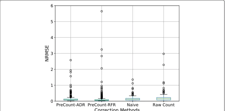
CCrtachieved anNRMSEof 0.15 for all test days in the count dataset. This indicates that PreCount’s correction methods achieved a 58% error reduction for theMALLbuilding case. Lastly, for theLIBRARYbuilding case, theADR,RFRand the naive correction meth-ods achieved anNRMSEof 0.15, 0.14 and 0.17 respectively whileCCrtachieved anNRMSE
of 0.22 for all test days in the count dataset. This indicates that both regression methods achieved a 36% error reduction for theLIBRARYbuilding case.
In all the building cases, theRFRmodel achieved better error reduction than theRFR model. This is because, the perfect fit of the Adaboost meta-estimator may have over-fitted the correction model such that it is less generalization to new correction cases.
Ground truth result
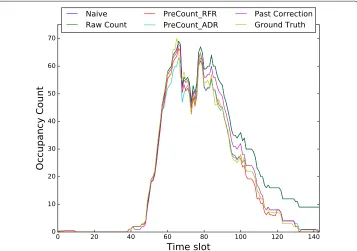
Figure9highlights the performance of PreCount’s correction methods (ADRandRFR), compared to the naive approach,CCrt, andCCpfor the 1-day ground data in theOFFICE
building case. For this evaluation case, the ADR, RFR, CCp, and the naive approach
achieved anNRMSEof 0.11, 0.10, 0.12 and 0.31 while theCCrtachieved anNRMSEof 0.31.
Fig. 8Boxplot showing the performance of each correction method forLIBRARYbuilding case
This indicates that the PreCount correction method achieved a 68% error reduction com-pared to the naive approach andCCrt and, a slight improvement over CCp. Also from
this evaluation, it can be observed that none of PreCount’s correction method violates the requirements stipulated by the United States Department of Energy (US Department of Energy2017).
Comparison between building cases
In this section, we discuss the variation in the results obtained from all building cases. In Table3, we summarize the performance of all correction methods for datasets obtained from all building cases. From this table, it can be observed that the error reduction
Table 3A table comparing the evaluation results for all building cases Correction methods Building cases
UNIVERSITY MALL LIBRARY OFFICE
Raw count 1.60 0.15 0.22 0.31
Naive 1.53 0.12 0.17 0.12
PreCount_RFR 0.62 0.05 0.14 0.10
PreCount_ADR 0.85 0.09 0.15 0.11
Sampling rate (Minutes) 1 15 60 1
Error reduction(%) 60% 58% 36% 68%
from theUNIVERSIT Y,MALL, andOFFICEbuildings are more significant compared to the LIBRARYbuilding case. The primary cause of this disparity is the rate at which the count
datasets are a sample from the camera sensors. For instance inLIBRARYbuilding case, PreCount has fewer points to corrects over the course of the evaluation period because of the high sampling rate compared to other building cases. Also, the aggregation over a longer sampling period reduces the variability in the dataset, and such variability will usually facilitate the training of a more robust regression model.
Training dataset size
The results in the previous section have used the entire training dataset in the training phase of PreCount. However, there are instances where there are limited training data such as cases where counting devices have recently been deployed. For these cases, we investigate the accuracy of PreCounts, and we hypothesize that increasing the size of the training dataset should increase the accuracy of PreCount.
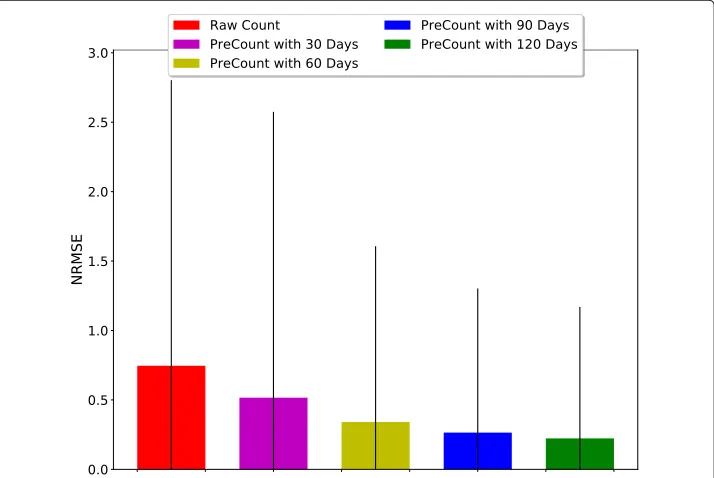
In Fig.10, we varied the size of the training dataset for theMALLbuilding case from 30 days to 120 days with a unit step of 30 days, and we employ a 95% confidence inter-val for theNRMSE. Also, we compared theNRMSEofCCrtwith theNRMSEof varying size
of the dataset. From Fig.10, training datasets with sizes 30, 60, 90 and 120 days achieved anNRMSEof 0.52, 0.34, 0.26 and 0.22 respectively compared toCCrt that has anNRMSE of 0.74. It can be observed that as the size of the training dataset increased, theNRMSE reduced i.e. the accuracy of PreCount increased over time. Also, with just 30 days of training data, PreCount achieved over 30% increase in accuracy compared toCCrt.
Discussion
The evaluation results presented in the four evaluation cases documents the merit of PreCount for performing count correction in real-time. From the overall performance in “Overall performance” section, PreCount achieved a 60%, 58% and 36% error reduction in theUNIVERSIT Y,MALLandLIBRARYbuilding respectively. The ground truth result in “Ground truth result” section shows a 68% count error reduction in anOFFICEbuilding. With the results obtained from the varying training sizes of the dataset in the “Training dataset size” section, PreCount could achieve as high as 30% error reduction with just 30 days of the training dataset. While the accuracies obtained from PreCount are signif-icant, these accuracies are achieved within the range of some of the highlighted feature sets in the “Feature analysis” section. Some of these feature sets were motivated from previous literature and are known contributors to erroneous counts, especially in cam-era technology. However, no previous litcam-erature enabled real-time count correction as enabled by PreCount. In this section, we discuss some of the limitations in this work, and we highlight some improvement opportunities to achieve better error detection and correction accuracy.
Firstly, PreCount assumes that there are available datasets for formulating the feature sets described in the “Feature analysis” section. However, in some locations, such datasets are not readily available. To address this concern, it could be relevant to perform a fea-ture ranking analysis alongside the feafea-ture correlation for all presented feafea-ture sets. This can be done in the training phase of PreCount with methods such as principal compo-nent analysis (PCA) or single value decomposition (SVD) to determine what correction accuracy is expected with the inclusion or exclusion of each feature group.
Also in Fig.10, we presented that increasing the size of the training dataset increases correction accuracy. However, it should be noted that as the size of training datasets increases, the time complexity for generating PreCount correction models also increases linearly. Therefore, a trade-off that maximizes both the accuracy for estimating count errors and estimation speed should be investigated to ensure that the latency for correct-ing real-time counts are minimal for each domain application.
Conclusions
a real-time count correction problem. Thirdly, we evaluate the performance PreCount’s correction methods using three evaluation cases and with datasets from four building cases. The first two evaluation cases benchmark the overall performance of both cor-rection methods withCCpdataset from the first three building and ground truth data
from the last building respectively. The third evaluation case evaluates the performance of PreCount with varying sizes of training data. Lastly, we present the results from all the evaluation cases. The results from the first evaluation case indicate thatRFR outper-formsADRin all building cases. In the second evaluation case, both correction methods achieved a maximum error reduction of 68% compared toCCrt and the naive approach
and, a slight improvement overCCp. And in the third evaluation case, PreCount achieved
an increasing accuracy as the training dataset increases and with just 30 days of training data, PreCount achieved an error reduction of over 30% when compared to raw counts. From the foregoing, PreCount can reliably produce high fidelity correction of occupant counts in real-time. Also, PreCount can achieve significant error reduction when limited training data are available for training.
In conclusion, given that PreCount achieves high fidelity correction ofCCrt, PreCount
can facilitate a number of pervasive and real-time applications that spans several domains such as disaster prevention and management, building energy management, and queue management in retail stores.
Funding
This work is supported by Innovation Fund Denmark for COORDICY (4106-00003B).
Availability of data and material Please contact author for data requests.
Authors’ contributions
FCS carried out the implementation and design of the occupant estimation algorithm and drafted the manuscript. MBK assisted in formulating the idea of the study, participated in the design of the algorithm and helped to draft the manuscript. All authors read and approved the final manuscript.
Competing Interest
The authors declare that they have no competing interests.
Publisher’s Note
Springer Nature remains neutral with regard to jurisdictional claims in published maps and institutional affiliations.
Received: 26 March 2018 Accepted: 2 August 2018
References
Arendt K, Ionesi A, Jradi M, Singh AK, Kjærgaard MB, Veje C, Jørgensen BN (2016) A building model framework for a genetic algorithm multi-objective model predictive control. In: 12th REHVA World Congress CLIMA 2016. Aalborg University, Department of Civil Engineering, Aalborg
Beltran A, Erickson VL, Cerpa AE (2013) Thermosense: Occupancy thermal based sensing for hvac control. In: ACM, BuildSys’13. ACM, NY, USA. pp 11:1–11:8
Caucheteux A, Sabar AE, Boucher V (2013) Occupancy measurement in building: A litterature review, application on an energy efficiency research demonstrated building. Int J Metrol Qual Eng 42:135–144
Chang W-K, Hong T (2013) Statistical analysis and modeling of occupancy patterns in open-plan offices using measured lighting-switch data. Build Simul 6:23–32
Christensen K, Melfi R, Nordman B, Rosenblum B, Viera R (2014) Using existing network infrastructure to estimate building occupancy and control plugged-in devices in user workspaces. Int J Commun Netw Distrib Syst 12(1):4–29 Ekwevugbe T, Brown N, Pakka V, Fan D (2013) Real-time building occupancy sensing using neural-network based sensor
network. In: Digital Ecosystems and Technologies (DEST), 2013 7th IEEE International Conference on. IEEE, Menlo Park. pp 114–119
Erickson VL, Carreira-Perpiñán MÁ, Cerpa AE (2011) Observe: Occupancy-based system for efficient reduction of hvac energy. In: Information Processing in Sensor Networks (IPSN), 2011 10th International Conference on. IEEE, Chicago. pp 258–269
Hutchins J, Ihler A, Smyth P (2007) Modeling count data from multiple sensors: A building occupancy model. IEEE, St. Thomas
Ihler A, Hutchins J, Smyth P (2006) Adaptive event detection with time-varying poisson processes. In: ACM, KDD ’06. ACM, New York, NY, USA. pp 207–216
Jensen T (2016) Open Data aarhus.https://www.odaa.dk/dataset/taellekamera-pa-dokk1.Accessed 3 Apr 2017 Jones E, Oliphant T, Peterson P, et al. (2001) SciPy: Open source scientific tools for Python.http://www.scipy.org/.
Accessed 24 Nov 2015
Kamthe A, Jiang L, Dudys M, Cerpa A (2009) Scopes: Smart cameras object position estimation system. In: EWSN ’09. Springer-Verlag. pp 279–295
Kennedy S (2010) Astral python library.https://pypi.python.org/pypi/astral/0.8.1. Accessed 3 Apr 2017 Kjærgaard MB, Johansen A, Sangogboye F, Holmegaard E (2016) Occure: An occupancy reasoning platform for
occupancy-driven applications. In: 2016 19th International ACM SIGSOFT Symposium on Component-Based Software Engineering (CBSE) IEEE, Venice. pp 39–48
Kjærgaard MB, Arendt K, Clausen A, Johansen A, Jradi M, Jørgensen BN, Nelleman P, Sangogboye FC, Veje C, Wollsen MG (2016) Demand response in commercial buildings with an assessable impact on occupant comfort. In: Smart Grid Communications (SmartGridComm), 2016 IEEE International Conference on. IEEE, Sydney. pp 447–452
Kuutti J, Saarikko P, Sepponen RE (2014) Real time building zone occupancy detection and activity visualization utilizing a visitor counting sensor network. In: IEEE. IEEE, Porto. pp 219–224
Pedregosa F, Varoquaux G, Gramfort A, Michel V, Thirion B, Grisel O, Blondel M, Prettenhofer P, Weiss R, Dubourg V, Vanderplas J, Passos A, Cournapeau D, Brucher M, Perrot M, Duchesnay E (2011) Scikit-learn: A random forest regressor.http://scikit-learn.org/stable/modules/generated/sklearn.ensemble.RandomForestRegressor.html. Accessed 3 Apr 2017
Pedregosa F, Varoquaux G, Gramfort A, Michel V, Thirion B, Grisel O, Blondel M, Prettenhofer P, Weiss R, Dubourg V, Vanderplas J, Passos A, Cournapeau D, Brucher M, Perrot M, Duchesnay E (2011) Scikit-learn: An adaboost regressor. http://scikit-learn.org/stable/modules/generated/sklearn.ensemble.AdaBoostRegressor.html.Accessed 3 Apr 2017 Pedregosa F, Varoquaux G, Gramfort A, Michel V, Thirion B, Grisel O, Blondel M, Prettenhofer P, Weiss R, Dubourg V,
Vanderplas J, Passos A, Cournapeau D, Brucher M, Perrot M, Duchesnay E (2011) Scikit-learn: Machine learning in Python. JMLR 12:2825–2830
Sangoboye FC, Kjærgaard MB (2016) Plcount: A probabilistic fusion algorithm for accurately estimating occupancy from 3d camera counts. In: Proceedings of the 3rd ACM International Conference on Systems for Energy-Efficient Built Environments, BuildSys ’16. ACM, New York, NY, USA. pp 147–156
Sangogboye FC, Kjærgaard MB (2017) Promt: predicting occupancy presence in multiple resolution with time-shift agnostic classification. Comput Sci Res Dev:1–11
Shan S, Gao W, Cao B, Zhao D (2003) Illumination normalization for robust face recognition against varying lighting conditions. In: 2003 IEEE International SOI Conference. Proceedings (Cat. No.03CH37443) IEEE, Nice. pp 157–164 US Department of Energy (2017) Advanced Research Projects Agency Energy. Saving energy nationwide in structures
with occupancy recognition (sensor). https://arpa-e-foa.energy.gov/FileContent.aspx?FileID=709732a8-c6f2-410f-95a8-21de1752e259.Accessed 13 Sept 2017
Submit your manuscript to a
journal and benefi t from:
7 Convenient online submission
7 Rigorous peer review
7 Immediate publication on acceptance
7 Open access: articles freely available online
7 High visibility within the fi eld
7 Retaining the copyright to your article