R E S E A R C H
Open Access
The bow tie structure of the Bitcoin
users graph
Damiano Di Francesco Maesa
1*, Andrea Marino
2and Laura Ricci
2*Correspondence:
[email protected] 1Department of Computer Science and Technology, University of Cambridge, William Gates Building, Cambridge, UK
Full list of author information is available at the end of the article
Abstract
The availability of the entire Bitcoin transaction history, stored in its public blockchain, offers interesting opportunities for analysing the transaction graph to obtain insight on users behaviour. This paper presents an analysis of the Bitcoin users graph, obtained by clustering the transaction graph, to highlight its connectivity structure and the
economical meaning of the different obtained components. In fact, the bow tie structure, already observed for the graph of the web, is augmented, in the Bitocoin users graph, with the economical information about the entities involved. We study the connectivity components of the users graph individually, to infer their macroscopic contribution to the whole economy. We define and evaluate a set of measures of nodes inside each component to characterize and quantify such a contribution. We also perform a temporal analysis of the evolution of the resulting bow tie structure. Our findings confirm our hypothesis on the components semantic, defined in terms of their economical role in the flow of value inside the graph.
Keywords: Bitcoin, Blockchain, Graph analysis, Bow tie, Complex networks
Introduction
This paper presents an analysis of the Bitcoin users graph, obtained by heuristic clustering of the Bitcoin transaction graph. In the users graph nodes represent Bitcoin users and edges model the flow of value between them. This graph contains information which may be used to conduct rich analyses. Indeed, the nodes are augmented with the users balance and the edges are weighted according to the Bitcoin value exchanged. Moreover, the information contained in the Blockchain reports also the creation dates of each edge, and this can be exploited to perform a set of temporal analysis.
The analysis takes inspiration from the seminal paper (Broder et al.2000), introduc-ing the concept of a bow tie structure for the graph representintroduc-ing the Web (subsequently refined in Meusel et al. (2014); Donato et al. (2008)). In this graph, each node corresponds to a web page and two nodes are connected by a direct arc whether there is an hyperlink from one to the other. Differently from the graph collected by Broder et al. (2000), we have a richer set of information which allows us to link the structure of the graph with the economical activities of the users.
The macroscopic representation of the graph as a bow tie derives from the partitioning of the graph in separate components according to the connectivity of its nodes, i.e. each node is assigned to a given component according to its reachable nodes set. The nodes in the biggest strongly connected component are calledSCC. The remaining nodes reaching
(resp. reached by) the ones in theSCCare calledIN(resp.OUT). The other nodes in the biggest weakly connected component are calledTUBE,TENDRIL, orFRINGE(see “Formal definitions and method” section for the formal definition), and the remaining nodes of the graph are calledDISCONNECTED.
In the first part of the paper, we support our conjecture that each component gives a different contribution to the graph from an economical point of view. In this sense, the macroscopic bow tie structure of the graph reflects the flow of value between the different components in the Bitcoin economy. In such light, we might think of theSCC
component as the dynamic core of the economic community, the component where value exchanges take place. Following the same model, the INcomponent would contain the nodes moving value towards theSCCandOUT would represent the set of nodes where value is credited from theSCC. We verify our conjecture on actual data, proving that the purely topological structure reflects on the different measures we consider to monitor the economical activity of the nodes.
In the second part of the paper, we perform a temporal analysis, studying how the different components change over time. Since by our hypothesis the topology is linked to the economical activity, our observations give also insights on how said eco-nomical activity changes over time from a macroscopic point of view in the Bitcoin economy.
We have presented a preliminary evaluation of the Bitcoin User graph connectivity structure in Di Francesco Maesa et al. (2018b). Beside a general revision and improve-ment, this paper extends our previous work in the following directions:
• we include a “Data acquisition” section, to better explain how the dataset has been acquired and built;
• we provide the high level definition of the algorithm used to assign roles to the nodes in the graph (Formal definitions and method);
• we double the set of measures performed on the connectivity components, by including a set of measures regarding cluster lifespans. We define such new measures, comment their relevance regarding the components and present a new graph to outline the most interesting result (The bow tie structure of the Bitcoin users graph);
• we extend the temporal analysis of the graph components not only by including and commenting a new graph to corroborate our previous observations, but also by discussing more deeply node activity andDISCONNECTEDcomponent behaviour (Temporal analysis). A new set of experimental results is provided to support our considerations.
Fig. 1The bow tie structure of the Bitcoin users graph. For each component is shown its size (i.e. the number of nodes it contains) and the percentage of nodes it contains with respect to the whole graph. For readability the components are not scaled according to their relative sizes
Background and related work
Bitcoin (Nakamoto 2008) is a cryptocurrency relying on blockchain technology. This means that the entire history of the system is saved inside a secure and decentralised ledger (called blockchain) in an append only fashion. The blockchain defines the state of the system and each new block added to it contains an ordered set of transactions
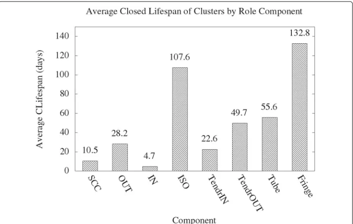
Fig. 3Average CLIFESPANvalues per role component as defined in “Evaluation of component metrics” section
expressing a state update. From an high level point of view it can be modelled as a map-ping of values to addresses, where transactions are the only tool available to change such mapping by transferring value between different addresses. This abstraction suf-fices for the scope of this paper, for more precise explanation of the Bitcoin protocol see Bonneau et al. (2015). Each transaction is many to many, i.e. it can have multiple addresses providing value to be spent as inputs (named multi-input transaction) and more than one address receiving part of such value as output. The couple (address, value) receiving a payment through a transaction is calledtransaction outputin the rest of this paper. Furthermore there exists a special transaction type, called coinbase, to reward a fixed value and some collected fees to somemineraddresses for each block. A miner is a voluntary validator node, willing to dedicate some computational power to take part into the distributed consensus algorithm behind the Bitcoin blockchain secu-rity guarantees. Since validating new blocks, i.e.mining, is a computationally intensive task, randomized rewards are proportionally assigned to miners. The rationality behind such rewards and the mining process is beyond the scope of this paper, for further reading see Bonneau et al. (2015). It suffices to say that newly generated value is con-stantly entered into the system through special transactions with no inputs (i.e. coinbase transactions).
all input addresses of a transaction belong to the same user (Nakamoto2008; Fergal and Harrigan2013). By parsing all transactions in the blockchain it is possible to build a trans-actions graph(representing value exchanges between addresses), that can be then refined into anusers graph(representing payments between approximated users) by applying the heuristic clustering.
Several analysis of the Bitcoin graph have been presented. Some of them only consider the transactions graph (Kondor et al.2014; Popuri and Gunes2016), but this may lead to less meaningful results due to the high number of different addresses that are con-trolled by the same user. Other analysis have been performed on the users graph (Ron and Shamir2013; Meiklejohn et al.2013; Androulaki et al.2013; Lischke and Fabian2016; Di Francesco Maesa D et al.2017; Di Francesco Maesa et al.2016a), as for our own study first presented in Di Francesco Maesa D et al. (2016b) and later expanded in Di Francesco Maesa et al. (2018a). Relying on the users graph instead of the transactions graph often results in more interesting insight, but the accuracy of the clustering step needs to be taken in account not to skew the analysis (Harrigan and Fretter 2016). Despite some efforts have been made trying to represent the Bitcoin users graph structure, mainly in the area of graph visualization (McGinn et al.2016), at the best of our knowledge no pre-vious work is available on its macroscopic bow tie structure analysis, as performed by this work.
Data acquisition
The analysis presented in this paper are performed on a set of snapshots of the Bitcoin users graph obtained from the dataset presented in Di Francesco Maesa et al. (2018a). For a detailed description of the dataset and tools used to retrieve it, the interested reader can refer to Di Francesco Maesa et al. (2018a), in this section we only highlight its character-istics more relevant to this work. We also remark how this work is based on the Bitcoin main chain, no forks of the Bitcoin official history are taken into account (such as the BitcoinCash one).
The temporal analysis is performed by considering a set of temporal snapshots of the users graph. For each temporal snapshot, the analysis is applied to the induced graph, which is the graph containing only transactions with a timestamp less than the considered cut-off timestamp, pruned of its periphery, i.e. by cutting-off nodes that only have one incoming arc. The main aim of this pruning is to penalize the nodes corresponding to users that just received a payment and might have had no time to spend it due to the artificial cut introduced by the time snapshot cut-off. Do note that the pruned nodes have no influence on the connectivity of the graph (because they only have a single incoming edge).
Finally, since each node of the graph corresponds to a cluster of addresses, in the fol-lowing we will use the term node and cluster interchangeably. We also remark how we use the termnodeaccording to the graph theory notation, i.e. a node belongs to the users graph and, in turn, it represents a set of addresses, not to be confused with anodeof the Bitcoin peer-to-peer communication network.
Formal definitions and method
Given the users graphG(V,E)obtained by the clustering heuristic of the Bitcoin transac-tions graph (see “Background and related work” section), we assign roles to the nodes in
Vfollowing the notation of Broder et al. (2000), and summarized in the well-known bow tie structure scheme shown in Fig.1. The role of a nodexis based on the set of nodes
xcan reach and that can reachx, as formalized next. In the following we refer toG∗as the undirected graph obtained symmetrizingG, i.e. obtained byGwithout considering the direction of the edges. Moreover, we callG−1as theinversegraph ofGobtained by
reverting the direction of all the edges ofG.
Definition 1Given a graph G(V,E), the role of the nodes in V is defined as follows.
• DISCONNECTED: nodes not connected to the giant connected component ofG∗. • SCC: nodes in the giant strongly connected component of G.
• IN: nodes not inSCCand able to reach the nodes in SCC. • OUT: nodes not inSCCand reachable by the nodes inSCC.
• TENDRIL: nodes not in the previous categories, that either can reach at least a node in OUT(TENDRILTOOUT) or can be reached by at least a node inIN
(TENDRILFROMIN), but not both.
• TUBE: nodes not inSCC, that can reach at least a node inOUT, and can be reached by at least one node in IN.
• FRINGE: nodes not in any of the previous categories.
The nodes having roleFRINGEinclude the ones which are connected toTENDRIL (even-tually using an undirected path). For instance, this is the case of a nodeyreachingx ∈ TENDRIL, wherexcan be reached byIN(i.e.x∈TENDRILFROMIN).
For the sake of completeness, we report here the linear algorithm we have used to assign to each node ofGits corresponding role. It should be remarked that, due to the size of the network, the reachability tests for sets of nodes have to be linear. We have addressed this task using aBFS(Breadth First Search) multi-source, which, given a set of nodesX, computes the set of nodes reachable from at least one node inX. Namely, aBFS multi-source is a modifiedBFSwhose starting queue is filled with all the nodes inX.
The resulting algorithm is shown in Algorithm1. It firstly starts computingG−1, G∗
and the connected components ofG∗to assign the labelDISCONNECTED. After this, the algorithm computes the strongly connected components ofGto assign the roleSCC. It then computes the nodes reachable from the nodes inSCC(assigning to them the role
OUT). This is done using a BFSmulti-source which marks the visited nodes. Similarly,
but using the symmetric graphG−1, the algorithm computes the nodes able to reach the nodes inSCC(assigning to them the role IN). At Lines11and12, the algorithm com-putes the nodes reachable fromINinG, assigning to them the roleTENDRIL. Finally, the nodes reachingOUT are computed: the ones who were reached also byINare labelled asTUBE, the other ones are labeled as TENDRIL. All the remaining nodes are labeled asFRINGE.
As a result, the following holds.
Lemma 1Given a graph G(V,E), Algorithm1computes the roles of all the nodes in V according to Definition1.
The bow tie structure of the Bitcoin users graph
Algorithm 1:Assigning roles to the nodes. Input : G(V,E)=a graph;
Output: r[v]=role of eachv∈V, with role in
{SCC,IN,OUT,TENDRIL,TUBE,FRINGE}
1 LetG−1be the inverse graph ofG
2 LetG∗be the symmetrized graph obtained byG
3 Compute the Giant Connected ComponentK∗ofG∗
4 forv∈V\K∗dor[v]←DISCONNECTED
5 forv∈Vdor[v]←null
6 Compute the Giant Strongly Connected ComponentKofG
7 forv∈Kdor[v]←SCC
8 mark←B F S-M U L T I-S O U R C E(G,SCC)
9 forv s.t. mark[v]=true and r[v]=nulldor[v]←OUT
10 mark←B F S-M U L T I-S O U R C E(G−1,SCC)
11 forv s.t. mark[v]=true and r[v]=nulldor[v]←IN
12 mark←B F S-M U L T I-S O U R C E(G,IN)
13 forv s.t. mark[v]=true and r[v]=nulldor[v]←TENDRIL
14 mark←B F S-M U L T I-S O U R C E(G−1,OUT)
15 forv s.t. mark[v]=truedo
16 ifr[v]=TENDRILthenr[v]←TUBE
17 ifr[v]=nullthenr[v]←TENDRIL
18 forv s.t. mark[v]=nulldor[v]←FRINGE
19 returnr
20 FunctionB F S-M U L T I-S O U R C E(G(V,E),)
21 queue← ∅
22 forv∈Vdomark[v]←false
23 forv∈V s.t. r[v]=do
24 queue.enqueue(v)
25 mark[v]←true
26 whilequeue not emptydo
27 w←queue.removeFirst()
28 forv∈N(w)do
29 if mark[v]=falsethen
30 queue.enqueue(v)
31 mark[v]←true
32 returnmark
semantic explanation of the role of each component can be inferred from the way the Bitcoin protocol works.
(2000), whose nodes are web pages and whose edges represent hyperlinks between them1. The results about the web graph presented in Broder et al. (2000) show the IN, OUT, andTENDRILcomponents all with almost same dimensions (21.29%, 21.29% and 21.52% respectively), while theSCCcomponent is slightly bigger (27.74%) andDISCONNECTED
about one third the size of them (8.24%). In comparison in Fig.1theSCCcomponent is dominant over all the others (containing 86.36% of all the nodes in the graph), the next component by size isDISCONNECTED(9.08%) followed byOUT(2.48%) andIN(2.06%),
with the size of all other components almost irrelevant. We should remark that the com-ponent sizes distribution reliability has been questioned as a measure in the literature, since it is thought to depend on the web crawler adopted. For example in Meusel et al. (2014), the authors state that “While it is always possible to compute the components of the bow tie of Broder et al. (2000), the proportion of the components is not intrinsic”. In the same paper the computed component sizes differ greatly from Broder et al. (2000) (SCC51.28%,IN31.96%,OUT6.05%,TENDRIL4.61% andDISCONNECTED5.84%),
prob-ably both because of the different crawler used and because of the different time of data collection.
Economical interpretation of the graph components In the remaining part of this section, we link the bow tie structure to the economical activity of the nodes involved in the different components. We aim to show thatSCCrepresents the center of the econom-ical activity, whereINnodes move value towards theSCCandOUTnodes correspond to nodes with value credited from theSCC.
In this scenario OUT would contain the yet unspent outputs from the SCC, either because the owner did not have time to spend them before the data acquisition time cut-off or because they were deposited for cold storage. TheIN nodes instead should represent mainly miners obtaining newly minted value in the form of mining rewards (see “Background and related work” section). Such value is then injected (i.e. spent) in the main economy of Bitcoin, represented by the SCC. In fact a new node is created in the graph as soon as its corresponding cluster in the blockchain receives a pay-ment, so, inside the giant weakly connected component, value flows by design from nodes with no incoming arcs (that can only be part of IN) through multiple
interme-diate nodes until they reach nodes with no outgoing arcs (that can only be members of OUT). Of course this is not in general the only case, since the same node can receive both new value as mining rewards as well as payments (and so arcs) from other nodes. In this scheme TENDRILFROMIN (TENDRILTOOUT) are anomalies that send value to (receive value from) nodes not part of the main economy (i.e. outside the SCC). Similarly TUBE nodes transmit value from IN to OUT bypassing the SCC
completely.
To get a first insight supporting such hypothesis we used a dataset of 12 413 deanonymized nodes (with identities obtained from (Blockchain Info Tags 2019)), i.e. clusters containing an address associated to a known real world entity, to map them to the relative component in the graph. Deanonymized nodes were only found inside the four main components (SCC,IN,OUT and DISCONNECTED). In particular IN only contained three nodes representing known entities. By manual inspection we found these entities to belong to two minor miners2 part of pools and a mining pool3. Conversely most of
observed in Di Francesco Maesa et al. (2018a) to be the most central nodes in the graph, are part of theSCC. E.g. consider Table 4 in Di Francesco Maesa et al. (2018a) show-ing the ten most central nodes accordshow-ing to Harmonic, Eigenvector and Page-Rank node centrality.
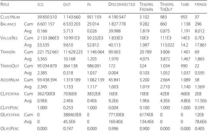
Evaluation of component metrics
To better understand the type of nodes with different roles we evaluated the following metrics with respect to each role. We do remark how the introduced measures, with the exception of CLUSTNUM, are not classical graph measures, and, as such, are independent from the structure of the graph considered.
• CLUSTNUM: represents the number of clusters for each role component, since clusters correspond to graph nodes, it is the same as number of nodes for each component.
• BALANCE: measures the current (at data collection time) balance of a cluster (i.e. sum of balances of all its addresses).
• VALUEREC: expresses the total value received during a cluster lifespan, or up to the time of data collection if the cluster is still active. It is defined as the sum of all payments received. This measure helps to point out clusters with small current balance (for example zero), that have owned a lot of value in the past.
• TRANSIN: represents the number of payments received by a cluster (coinbase rewards included). This measure is useful in estimating the economical importance of a cluster in the way of collecting payments.
• TRANSOUT: measures the number of payments done by a cluster. It is computed as the number of transactions originated from a cluster. This measure represents the economical importance of a cluster as its weight in issuing payments. Note that both TRANSINand TRANSOUTmeasures the in and out-degrees of the clusters, including self-loops and multi-edges. These kind of edges happen whenever two addresses of the same cluster exchange money or there is a repeated payment between two clusters.
We remark how this measure is not the same as the number of arcs incoming and outgoing, respectively, in the graph. In fact, due to the addresses clustering step, some transactions may become self loops or repeated arcs. Furthermore, repeated arcs may naturally be present between addresses, not consequence of our clustering. Since both self loops and repeated arcs do not influence the graph connectivity they are ignored during our connectivity analysis. This is why the two measures can vary greatly from nodes indegree and outdegree respectively.
• ADDRNUM: counts the number of addresses in a cluster. This measure can be used to indirectly estimate the cluster activity.
role component. Do note that by timestamp of a transaction we mean the timestamp of the block such transaction is part of in the blockchain.
• CLIFEPERC: represents the fraction of clusters in a given role component that have a closed lifespan, i.e. the number of clusters making at least one payment divided by the number of clusters in that component.
• OLIFESPAN: measures the lifespan, in milliseconds, of a cluster that never performs a payment. We name this measureopen lifespan because the cluster only has a creation date. Since there is no last activity date for such clusters we measure their lifespan as time passed from their creation date to the data collection cut-off. Same as for CLIFESPAN, the average of this value is computed among open lifespan clusters only in each role component.
• OLIFEPERC: represents the fraction of clusters in a given role component that have an open lifespan. As a consequence of their definitions it holds that
OLifePerc+CLifePerc=1for each role component.
The cumulative (i.e. the sum of the values of all nodes with the same role) and average (i.e. the cumulative value divided by the number of nodes with a given role) values of the introduced measures for each component are presented in Table1. To better understand the contribution of each role component to each measure (excluding lifespan ones) we also depict the percentages of the cumulative values with respect to the cumulative value for the entire graph (ignoring role components) in Fig.2.
As a side remark, since Table1reports the number of addresses in each component, by considering the ratio between the cumulative value of each measure in each compo-nent and the number of addresses in that compocompo-nent, one can characterize the average behaviour of the addresses independently from the clustering phase. This allows to obtain,
Table 1Cumulative and Average values of the introduced measures for each role component
ROLE SCC OUT IN DISCONNECTED TENDRIL
FROMIN
TENDRIL
TOOUT
TUBE FRINGE
CLUSTNUM 39 850 510 1 143 660 951 159 4 190 547 5 102 983 955 37 BALANCE Cum 6 601 157 6 533 203 25 014 1 827 778 9 282 860 1 138 296
Avg 0.166 5.713 0.026 39.988 1.819 0.875 1.191 8.012 VALUEREC Cum 2 133 386E3 10 991E3 50 232E3 1 833E3 10E3 111E3 14E3 0.7E3 Avg 53.535 9.610 52.812 40.113 1.987 113.022 14.2 17.861 TRANSIN Cum 221 752 661 11 629 223 1 146 064 90 063 20 789 3 806 1 401 69
Avg 5.565 10.168 1.205 1.970 4.075 3.872 1.467 1.865 TRANSOUT Cum 95 034 879 364 138 986 091 172 524 1 034 990 22
Avg 2.385 0.318 1.037 0.004 0.103 1.052 1.037 0.595 ADDRNUM Cum 93 438 394 1 319 189 1 062 139 45 841 5 200 2 664 1 089 58
Avg 2.345 1.153 1.117 1.003 1.019 2.710 1.140 1.569 CLIFESPAN Cum 362700E8 7036E8 3832E8 16E8 10E8 42E8 46E8 2E8
Avg 0.9E6 2.4E6 0.4E6 9.2E6 1.9E6 4.3E6 4.8E6 11.5E6 CLIFEPERC 1.000 0.253 1.000 0.004 0.100 1.000 1.000 0.595 OLIFESPAN Cum 0 388463E8 0 77130E8 6174E8 0 0 12E8
Avg 0 45.5E6 0 169.4E6 134.4E6 0 0 78.6E6
OLIFEPERC 0.000 0.747 0.000 0.996 0.900 0.000 0.000 0.405
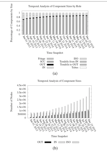
Fig. 5Temporal analysis of role component size percentages over the whole graph (a), temporal analysis of component sizes restricted to the three most significant components excluding the dominatingSCConly (i.e.
OUT,INandDISCONNECTED) (b). For the precise GMT time snapshot dates, see Di Francesco Maesa et al. (2018a)
for instance, the average balance and the average value of the incoming transactions of the addresses present in each component.
Interestingly, we will show how the above measures, not dependent from the topology of the graph, are consistent with the topological partition found.
Clusters density From Fig.2we can observe how ADDRNUMfollows a distribution
average values for such measure in Table 1, we can note how, among the four main components (SCC,IN,OUTandDISCONNECTED),SCCis the only one to exhibit a value sensibly greater than one. TheDISCONNECTEDcomponent in particular exhibits a value very close to one, meaning that most of its clusters are actually addresses singletons. The fact that nodes in theSCChave the greatest average value for such measure supports our hypothesis that it contains the really active clusters of the economy.
Cluster lifespans First of all we remind that the lifespan values are computed from the block timestamps. The timestamp of each block is chosen by the miner actu-ally creating such block. Since there is no concept of universal clock, the timestamps can be inconsistent between adjacent blocks, i.e. a given block can have a times-tamp lower than a preceding block. As such, in few cases, the lifespan of a node could be negative. To avoid such problem we have introduced a lower bound of zero for the lifespans, i.e. nodes with negative lifespan are corrected to zero. We do remark how a lifespan of zero is, in general, a valid one, since it might represent a cluster receiving its first transaction and creating all its outgoing payments inside a single block.
From the values of OLIFEPERCand CLIFEPERCshown in Table1we can derive inter-esting considerations on clusters activity depending on the component they belong to. Obviously, 100% of clusters inSCC,IN,TENDRILTOOUTandTUBEhave a closed lifespan (i.e. they performed at least one payment). This is a direct consequence of how such com-ponents are defined. Conversely more than 99% of clusters inDISCONNECTEDhave an open lifespan, meaning that they have never spent the value received. This is consisted with our assumption that they represent isolated users with little to no economical inter-action between themselves. Similarly about 75% of clusters inOUTnever spend the value received (do note that nodes inOUTcan only transfer their value to other nodes inOUT), supporting our hypothesis on the role of clusters in such component.
Figure3depicts the average values of CLIFESPAN, i.e. the average time that clusters remain active, from Table1, expressed in days instead of seconds. We can see from the figure howINandSCCcontain the most short lived clusters (on average), while clusters in
OUTwith a closed lifespan remain active for about three times longer. This is consistent
with our assumption that INclusters pay out the value received quickly to SCC, while
OUTclusters contain temporary storage of value not immediately spent (and not as fast
as it happens in theSCC). Moreover, by looking at the average OLIFESPANof clusters in
OUTwe can measure the average time (i.e. age) of value inOUTstill waiting to be spent.
Clusters that never have spent their value inOUThave been waiting about 526 days (i.e.
about one and a half years) on average. Even if this value encompasses also the value that has simply been credited too soon to be spent (i.e. too close to the data collection cut-off )4, it can still be considered as lower value for average age of funds kept in cold storage or forgotten. Computing the same value for theDISCONNECTEDcomponent from Table1, we obtain an average age of approximately 1960 days, i.e. about five years and an half of funds inactivity (out of the approximately seven years span of the data), consistent with the assumed semantic of the component.
results. We can observe in Fig.2the marked discrepancy between the current balance and total value received by clusters. In fact even if theSCCdominates all measures in the figure, including the cumulative value received by its clusters, it also shows a surprisingly relatively low cumulative current balance. The proportional high value received indicates how value is mostly exchanged inside theSCC, while the low current balance indicates how a big part of such value is in the end credited to the clusters in theOUTcomponent, behaviour explained by our conjecture.
Coinbase transactions To better understand the flow of value in the graph we also performed a study on the presence of coinbase transactions (see “Background and related work” section) in clusters depending on their role. In particular we mea-sured NUMCOINB, as the number of transaction outputs (i.e. payments) received by clusters from coinbase transactions, UNIQUECOINB, as the number of clusters that received at least one payment from a coinbase transaction and BAL ANCE -COINB as the total value received by a cluster from coinbase transactions, i.e. the sum of all transaction outputs amounts received from coinbase transactions by the same cluster.
The fractions of the cumulative values by role component over the entire graph for these three measures are shown in Fig. 4, supporting our assumption on the IN com-ponent role. In fact we can note how the INcomponent contains most of the clusters that have received at least one coinbase transaction. Furthermore the evident difference between the first two columns in the same figure, i.e. the number of coinbase payments
received by nodes (NUMCOINB) and number of nodes that receive at least a coinbase transaction (UNIQUECOINB) tells us thatSCCactually contains less miners thanINeven if it receives more rewards. By looking at the third column, i.e. the cumulative value obtained from coinbase transactions (BAL ANCECOINB) we can also notice how theSCC
miners receive less value than the ones inINdespite receiving more individual rewards. This means that the miners inSCCnot only are fewer but also weaker. In fact if we com-pute the average coinbase payment (i.e. the cumulative value of the received rewards divided by the number of rewards received) received by the nodes in each component we find out the following values: 4.13 BTC for SCC, 0.35 BTC for OUT, 37.94 BTC forIN and 20.96 BTC forDISCONNECTED nodes. This shows how each nodes receiv-ing a coinbase reward in INreceives on average a reward nine times higher than the ones inSCC.
Final remarks We can conclude by saying that the introduced measures indeed sup-port our hypothesis about the semantic of the bow tie components. In particular, the assumption that theSCCrepresents the real economically active component is supported by the previous observations on clusters lifespan, density and balance. Especially so, by our remarks on the marked discrepancy between the current value hold and cumula-tive value received during time by the SCCclusters. At the same time, the balance and lifespan analysis corroborate our assumptions on theOUTandINcomponents, while the provided coinbase transactions analysis clearly supports our hypothesis on the INand
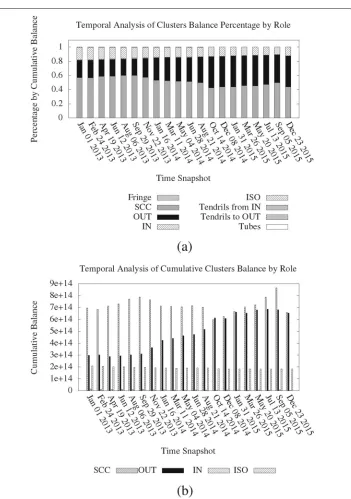
Fig. 6Temporal analysis of cumulative current balance percentages over the whole graph (a) and temporal analysis of cumulative current balance of the three most significant components (i.e.SCC,OUTand
DISCONNECTED) (b). For the precise GMT time snapshot dates, see Di Francesco Maesa et al. (2018a)
Temporal analysis
Such greater insight is always provided for free by design in current cryptocurrencies, because a node must have the possibility of recomputing and checking the entire history of transactions, starting from the very beginning, i.e. the genesis block.
To better understand the evolution of the components analysed in “The bow tie structure of the Bitcoin users graph” section we performed a temporal analysis of the con-nectivity of the graph. We choose to use the same timestamp cut-offs as Di Francesco Maesa et al. (2018a), i.e. to divide the timespan of our dataset in twenty temporal snap-shots all equal in duration except the first one. The first snapshot was chosen to be longer (four years unlike the approximately fifty five days of all other snapshots) to allow the graph to better represent a mature users usage, avoiding the anomalies and uncertainties of bootstrapping and early adoption years.
Measures We computed the same measures presented in “Evaluation of component metrics” section for each snapshot, obtaining their temporal behaviour. In the follow-ing we only show the evolution of the two we deem more interestfollow-ing: CLUSTNUM(i.e. component sizes, Fig.5), and BAL ANCE(Fig.6).
Component sizes Regarding the component sizes, we studied how nodes change their role over time. Concerning this, we remark that any older graph is a subgraph of a newer one, implying that nodes have a forced way of changing roles, ultimately favouring the
SCC component. In fact nodes with roleINorOUT can only change role by becoming
of roleSCC, since they already reach or are reachable, respectively from theSCC, and so any new edge that would cause them to change role can only result in them being able to both reach and being reachable by theSCCthus becoming nodes of roleSCCthemselves. Analogously, nodes belonging to aTENDRILcan only becomeIN(fromTENDRILFROMIN)
orOUT(fromTENDRILTOOUT),TUBEorSCC. Finally a node with roleTUBEcan change role to eitherIN,OUTorSCC. But once a node has roleSCCit can no longer change role. Of course, new nodes can get any role.
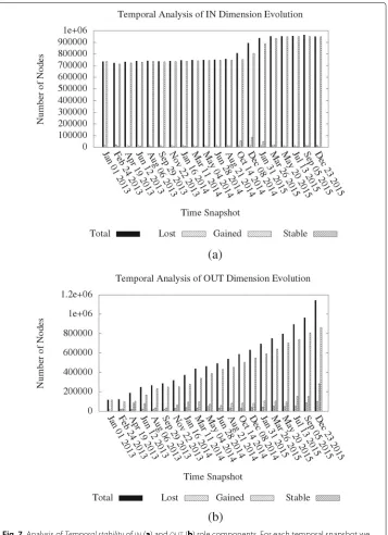
In order to measure how nodes change their role, we analysed thetemporal stabilityof the components. By “analysing thetemporal stabilityof a set of nodes” we mean counting the number of nodes that remain in the set between a temporal snapshot and the next as well as counting the number of nodes that leave or join the set. We show here the results for theINandOUTcomponents only, which are the two most relevant components by number of nodes in the biggest connected component (excluding theSCC).
Concerning the size of the different components over time, we observe the growth in proportional size of theSCCcomponent, mostly at the expenses of theINcomponent, as shown in Fig.5a. This behaviour is more evident in Fig.5b where the continue growth in terms of number of nodes of bothDISCONNECTED andOUTcomponents rapidly over-takes the initially largerINcomponent that, conversely, remains pretty much stable in size
over time5. The same consideration is even clearer by comparing Fig.7a and b. In fact theINcomponent, except for a moderate growth around the end of 2014, is pretty much
Fig. 7Analysis ofTemporal stabilityofIN(a) andOUT(b) role components. For each temporal snapshot we indicate withtotalthe number of nodes, withlostthe number of nodes that were present in the component during the previous temporal snapshot but are no longer present during the current snapshot, withgained
the number of nodes that were not present in the component during the previous temporal snapshot and withstablethe number of nodes present during both the previous and current snapshot. For the precise GMT time snapshot dates, see Di Francesco Maesa et al. (2018a)
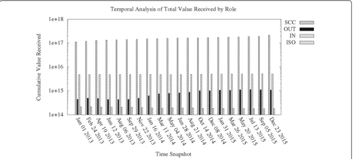
Fig. 8Temporal analysis of cumulative value received (i.e. VALUERECas defined in “Evaluation of component metrics” section) of the four most significant components (i.e.SCC,IN,OUTandDISCONNECTED). Do note the logarithmic scale. For the precise GMT time snapshot dates, see Di Francesco Maesa et al. (2018a)
balance of the component proportionally diminishes over time (since any value it holds is mostly transferred to theSCC), see Fig.6a.
Components cumulative balance The results obtained regarding the cumulative cur-rent balance values per component support our conjecture about the diffecur-rent economical roles of the different components. In fact, we can observe from Fig.6b that the current balance of theSCCremains somewhat stable, while the cumulative current balance ofOUT
increases over time. The same can be seen more clearly in Fig.6a where the percentage of value held by theOUTcomponent increases over time at the expenses of the other compo-nents (mainly theSCC). This is because more and more value actually passes and is used by the nodes in theSCC, but it is temporary (potentially for a long time in case of cold storage clusters) stored in theOUTcomponent in the form of currently unspent outputs. As a comparison we show in Fig.8the plot about the total value received over time for the four main components considered in Fig.6b. The behaviour ofSCC compared
to OUT is very different between Fig. 8. In fact, considering the cumulative received value over time SCCandOUT show a similar behaviour, as both approximately double their respective starting values (do note how the value received axis is in logarith-mic scale). Of course, SCC still moves value two orders of magnitude greater than
OUT, despite the final cumulative balance similarity. Such behaviour is also
consis-tent with the relatively high instability of the OUT component observable in Fig. 7b. In fact a relatively high dynamicity in the set is expected as the value stored in its nodes is spent (making them become a part of the SCCand leaving such value to cir-culate in the SCC) while, at the same time, new unspent outputs are created from theSCC.
Fig. 9Temporal analysis of the percentage ofactive nodes(a) andpassively active nodes(b) per role component respectively, during each temporal snapshot. For the precise GMT time snapshot dates, see Di Francesco Maesa et al. (2018a)
inactive, nodes that only receive payments. Arguably a node receiving payments might be considered an active part of an economy, so both receiving or issuing payments might be considered a sign of activity. Consequently we decided to evaluate both definitions, nam-ing a nodeactive during time t if the relative cluster performs at least one transaction during timet, andpassively active during time tif it isactive during time tor if the relative cluster is the beneficiary of at least one transaction output during timet. We do remark that the second definition is a generalization of the first, i.e. if a node isactiveduring a given timetit is alsopassively active. Furthermore, we remark that node activity is mea-sured at cluster level and not node level, so clusters with transactions between addresses inside themselves would still be considered active, even if, from a graph point of view, the corresponding arcs would result in ignored self loops. In Fig.9are shown the results for both definitions.
activity of theINcomponent at the end of 2014, consistent with what already observed in Fig.7a. From the comparison between Fig.9a and b, we can notice the unsurprisingly increased importance of theOUTcomponent if incoming payments are also considered as node activity.
DISCONNECTED component Finally we can formulate some considerations about the
DISCONNECTED component. In fact we can see from Fig.5b how the component size
increases over time, while Fig.6b tells us that the value it holds does not increase, it actu-ally decreases a little over time. This happens as few nodes get connected over time to the giant connected component by spending their value, and so changing component alto-gether. In fact the actual value hold by the component is only the one it has received from coinbase transactions. This is observable by comparing the second column of Fig.2with the third column of Fig.4: the current cumulative balance of the component matches with the amount received by coinbase transactions alone.
The increase in the size of the DISCONNECTED component is instead explainable by looking at the nodes it contains. In fact such component contains mostly singletons with no edges, representing clusters with one single address (as already observed in “Evaluation of component metrics” section). In fact 99.994% of all nodes in theDISCONNECTED com-ponent are isolated (i.e. they have no incoming or outgoing arcs) and have zero balance (i.e. they receive no value from coinbase transactions, and of course neither from regu-lar ones since they have no incoming arcs). Moreover theDISCONNECTEDcomponent is
proportionally relevant in Fig.9b, but it is not present in Fig.9a. This means that such isolated nodes appear in a transaction output, but they are not connected to other nodes (from nodes of components other thanDISCONNECTED) and have zero balance. A pos-sible explanation, that would satisfy all such anomalies, is that such nodes are created as recipients of special transaction outputs, carrying no value. Such special outputs are often used in the Bitcoin protocol to encapsulate arbitrary data inside the blockchain instead of transferring value (see Bartoletti and Pompianu (2017)). Since the script used in such transactions is none of the ones we decoded (see “Data acquisition” section) the resulting edge is not created, and the involved recipient address results in an isolated node.
Conclusions
In this paper we have presented a study of the connectivity defined components of the Bitcoin users graph following the bow tie structure presented in Broder et al. (2000). After formally defining the components and presenting the methods and dataset employed, we developed a semantic hypothesis on the economical role of each com-ponent. To verify our hypothesis, first we have defined a set of measures aimed at modelling node activity (focused on node balance, connections and lifespan). The aggre-gated values for all nodes part of each given component allowed us to derive macroscopic considerations. We have then performed a temporal analysis of the components evo-lution over time, by considering the evoevo-lution of the graph in a sequence of temporal snapshots.
Our analysis has shown that most of the economical exchanges are performed by the clusters belonging to theSCCcomponent of the graph, while the current balance is mostly contained in theOUTcomponent. Furthermore, we have discovered that most miners are
to those belonging to theSCCcomponent. These conjectures are further corroborated by the temporal analysis we performed.
We plan to extend our work in two different directions. First, we aim to better study the smallest components of the bow tie (i.e. TENDRILandTUBE) to aid possible deanonymization attempts. In fact, despite their small size, it is worth of investigation trying to understand why the nodes involved avoid the main economical community rep-resented bySCC. Second, it would be interesting to analyze other graph methodologies
for decomposing a network, studying the (eventual) corresponding economical meaning, extracting outlier users, and comparing them with the decomposition we have used, i.e. the bow tie in this paper. Finally, we are currently performing the same analysis for the graph obtained from other cryptocurrencies (e.g. Ethereum), with the goal of comparing the economies of the two cryptocurrencies.
Endnotes
1The terminology used in Broder et al. (2000) is the same as the one we use in this
paper.
2https://www.blockchain.com/btc/address/12jiD2M5aaQHcfREMF9XxbWxxD5EgUZ
wTw?filter=2 and https://www.blockchain.com/btc/address/1PH7zrvk16SQNCzarn39a Bt9S33NVMmHuH
3Halleychinahttps://cryptomining-blog.com/tag/halleychina/
4Even if we try to mitigate such bias by pruning the periphery, as explained in “Data
acquisition” section.
5We choose not to show theSCCin Fig.5b because its predominant size in the complete
graph would not allow to appreciate finer changes in the smaller components
Abbreviations
The Abbreviations introduced are explained in Definition1and regard the different connectivity components according to the bow tie structure of the Bitcoin users graph. In particular:
• DISCONNECTED: nodes not connected to the giant connected component of the undirected graph. • SCC: nodes in the giant strongly connected component.
• IN: nodes not inSCCand able to reach the nodes inSCC. • OUT: nodes not inSCCand reachable by the nodes inSCC.
• TENDRIL: nodes not in the previous categories, that either can reach at least a node inOUT(TENDRILTOOUT) or can be reached by at least a node inIN(TENDRILFROMIN), but not both.
• TUBE: nodes not inSCC, that can reach at least a node inOUT, and can be reached by at least one node inIN. • FRINGE: nodes belonging to the graph and not in any of the previous categories.
Acknowledgements
Not applicable.
Authors’ contributions
All authors have contributed equally to the paper. All authors read and approved the final manuscript.
Funding
Not applicable.
Availability of data and materials
Not applicable.
Competing interests
The authors declare that they have no competing interests.
Author details
1Department of Computer Science and Technology, University of Cambridge, William Gates Building, Cambridge, UK. 2Department of Computer Science, University of Pisa, Largo Bruno Pontecorvo 3, Pisa, Italy.
References
Androulaki E, Karame GO, Roeschlin M, Scherer T, Capkun S (2013) Evaluating user privacy in bitcoin. In: International Conference on Financial Cryptography and Data Security. Springer, Berlin. pp 34–51
Bartoletti M, Pompianu L (2017) An analysis of Bitcoin OP_RETURN metadata. In: International Conference on Financial Cryptography and Data Security. Springer, Cham. pp 218–230
Blockchain Info Tags (2019).https://blockchain.info/tags. Accessed 14 Mar 2019
Bonneau J, Miller A, Clark J, Narayanan A, Kroll JA, Felten EW (2015) Sok: Research perspectives and challenges for bitcoin and cryptocurrencies. In: 2015 IEEE Symposium on Security and Privacy. IEEE. pp 104–121
Broder A, Kumar R, Maghoul F, Raghavan P, Rajagopalan S, Stata R, Tomkins A, Wiener J (2000) Graph structure in the web. Comput Netw 33(1-6):309–320
Di Francesco Maesa D, Marino A, Ricci L (2016a) An analysis of the bitcoin users graph: inferring unusual behaviours. In: International Workshop on Complex Networks and their Applications. Springer, Cham. pp 749–760
Di Francesco Maesa D, Marino A, Ricci L (2016b) Uncovering the bitcoin blockchain: an analysis of the full users graph. In: 2016 IEEE International Conference on Data Science and Advanced Analytics (DSAA). IEEE. pp 537–546
Di Francesco Maesa D, Marino A, Ricci L (2018a) Data-driven analysis of bitcoin properties: exploiting the users graph. Int J Data Sci Anal 6(1):63–80
Di Francesco Maesa D, Marino A, Ricci L (2017) Detecting artificial behaviours in the bitcoin users graph. Online Soc Netw Media 3:63–74
Di Francesco Maesa D, Marino A, Ricci L (2018b) The graph structure of bitcoin. In: International Conference on Complex Networks and Their Applications. Springer, Cham. pp 547–558
Donato D, Leonardi S, Millozzi S, Tsaparas P (2008) Mining the inner structure of the web graph. J Phys A Math Theor 41(22):224017
Fergal R, Harrigan M (2013) An analysis of anonymity in the bitcoin system. In: Security and privacy in social networks. Springer, New York. pp 197–223
Harrigan M, Fretter C (2016) The unreasonable effectiveness of address clustering. In: 2016 Intl IEEE Conferences on Ubiquitous Intelligence & Computing, Advanced and Trusted Computing, Scalable Computing and
Communications, Cloud and Big Data Computing, Internet of People, and Smart World Congress (UIC/ATC/ScalCom/CBDCom/IoP/SmartWorld. IEEE. pp 368-373
Kondor D, Pósfai M, Csabai I, Vattay G (2014) Do the rich get richer? An empirical analysis of the bitcoin transaction network. PloS ONE 9(2):86197
Lischke M, Fabian B (2016) Analyzing the bitcoin network: The first four years. Futur Internet 8(1):7.https://doi.org/10. 3390/fi8010007
McGinn D, Birch D, Akroyd D, Molina-Solana M, Guo Y, Knottenbelt WJ (2016) Visualizing dynamic bitcoin transaction patterns. Big Data 4(2):109–119
Meiklejohn S, Pomarole M, Jordan G, Levchenko K, McCoy D, Voelker GM, Savage S (2013) A fistful of bitcoins: characterizing payments among men with no names. In: Proceedings of the 2013 conference on Internet measurement conference. ACM. pp 127–140
Meusel R, Vigna S, Lehmberg O, Bizer C (2014) Graph structure in the web—revisited: a trick of the heavy tail. In: Proceedings of the 23rd International Conference on World Wide Web. ACM. pp 427–432
Nakamoto S (2008) Bitcoin: A Peer-to-Peer Electronic Cash System
Popuri MK, Gunes MH (2016) Empirical analysis of crypto currencies. In: Complex Networks VII. Springer, Cham. pp 281-292 Ron D, Shamir A (2013) Quantitative analysis of the full bitcoin transaction graph. In: International Conference on
Financial Cryptography and Data Security. Springer, Berlin. pp 6–24
Publisher’s Note