R E S E A R C H
Open Access
Designing verbal autopsy studies
Gary King
1*, Ying Lu
2, Kenji Shibuya
3Abstract
Background:Verbal autopsy analyses are widely used for estimating cause-specific mortality rates (CSMR) in the vast majority of the world without high-quality medical death registration. Verbal autopsies–survey interviews with the caretakers of imminent decedents– stand in for medical examinations or physical autopsies, which are infeasible or culturally prohibited.
Methods and Findings:We introduce methods, simulations, and interpretations that can improve the design of automated, data-derived estimates of CSMRs, building on a new approach by King and Lu (2008). Our results generate advice for choosing symptom questions and sample sizes that is easier to satisfy than existing practices. For example, most prior effort has been devoted to searching for symptoms with high sensitivity and specificity, which has rarely if ever succeeded with multiple causes of death. In contrast, our approach makes this search irrelevant because it can produce unbiased estimates even with symptoms that have very low sensitivity and specificity. In addition, the new method is optimized for survey questions caretakers can easily answer rather than questions physicians would ask themselves. We also offer an automated method of weeding out biased symptom questions and advice on how to choose the number of causes of death, symptom questions to ask, and
observations to collect, among others.
Conclusions:With the advice offered here, researchers should be able to design verbal autopsy surveys and conduct analyses with greatly reduced statistical biases and research costs.
Introduction
Estimates of cause-specific morality rates (CSMRs) are urgently needed for many research and public policy goals, but high quality death registration data exists in only 23 of 192 countries [1]. Indeed, more than two-thirds of deaths worldwide occur without any medical death certification [2]. In response, researchers are increasingly turning to verbal autopsy analyses, a techni-que “growing in importance”[3]. Verbal autopsy studies are now widely used in the developing world to estimate CSMRs, disease surveillance, and sample registration [4-6], as well as risk factors, infectious disease outbreaks, and the effects of public health interventions [7-9].
The idea of verbal autopsy analyses is to ask (usually around 10-100) questions about symptoms (including some signs and other indicators) of the caretakers of randomly selected decedents and to infer from the answers the cause of death. Three approaches have been used to draw these inferences. We focus on the fourth
and newest approach, by King and Lu, which requires many fewer assumptions [10]. We begin by summarizing the main existing approaches. We then discuss our main contribution, which is in the radical new (and much easier) ways of writing symptom questions, weeding out biased symptoms empirically, and choosing valid sample sizes.
The first isphysician review, where a panel of (usually three) physicians study the reported symptoms and assign each death to a cause, and then researchers total up the CSMR estimates [11]. This method tends to be expensive, time- consuming, unreliable (in the sense that physicians disagree over a disturbingly large percen-tage of the deaths), and incomparable across populations (due to differing views of local physicians); in addition, the reported performance of this approach is often exag-gerated by including information from medical records and death certificates among the symptom questions, which is unavailable in real applications [12]. The sec-ond approach isexpert systems, where a decision tree is
constructed by hand to formalize the best physicians’
* Correspondence: [email protected]
1Institute for Quantitative Social Science, Harvard University, Cambridge MA
02138, USA
judgments. The result is reliable but can be highly inac-curate with symptoms measured with error [13,14].
The third approach is statistical classification and
requires an additional sample of deaths from a medical facility where each cause is known and symptoms are collected from relatives. Then a parametric statistical classification method (e.g., multinomial logit, neural net-works, or support vector machines) is trained on the hospital data and used to predict the cause of each death in the community [15]. These methods are unbiased only if one of two conditions hold. The first is that the symptoms have 100% sensitivity and specificity. This rarely holds because of the inevitable measurement error in survey questions and the fact that symptoms result from rather than (as the predictive methods assume) generate the causes that lead to death. A sec-ond csec-ondition is that the symptoms represent all predic-tive information and also that everything about symptoms and the cause of death is the same in the hospital and community (technically, the symptoms span the space all predictors of the cause of death and the joint distribution of causes and symptoms are the same in both samples [16]). This condition is also highly unlikely to be satisfied in practice.
Like statistical classification, the King-Lu method [10] is data-derived and so requires less qualitative judgment; it also requires hospital and community samples, but makes the much less restrictive assumption that only the distribution of symptoms for a given cause of death is the same in the hospital and community. That is, when diseases present to relatives or caregivers in simi-lar ways in the hospital and community, then the method will give accurate estimates of the CSMR. This is true even when the symptom questions chosen have very low (but nonzero) sensitivity and specificity, when these questions have random measurement error, when the prevalence of different symptoms and the CSMR dif-fer dramatically between the hospital and community, or if the data from the hospital are selected via case-control methods. Case-control selection, where the same num-ber of deaths are selected in the hospital for each cause, can save considerable resources in conducting the sur-vey, especially in the presence of rare causes of death in the community. The analysis (with open source and free software) is easy and can be run on standard desktop computers. In addition, so long as the symptoms that occur with each cause of death do not change dramati-cally over time (even if the prevalence of different causes do change), the hospital sample can be built up over time, further reducing the costs.
Conceptually, the King-Lu method involves four main advances (see Appendix A for a technical summary). First, King-Lu estimates the CSMR, which is the main quantity of interest in the field, rather than the correct
classification of any individual death. The method gener-ates unbiased estimgener-ates of the CSMR even when the percent of individual deaths that can be accurately clas-sified is very low. (The method also offers a better way to classify individual deaths, when that is of interest; see Appendix A and [[10], Section 8].) Second is a generali-zation to multiple causes of the standard “back
calcula-tion” epidemiological correction for estimating the
CSMR with less than perfect sensitivity and specificity [17,18]. The third switches“causes”and“effects” and so it properly treats the symptoms as consequences rather than causes of the injuries and diseases that lead to death. Since symptoms are now the outcome variables, it easily accommodates random measurement error in survey responses. The final advance of this method is dropping all parametric modeling assumptions and switching to a fully nonparametric approach. The result is that we merely need to tabulate the prevalence of dif-ferent symptom profiles in the community and the pre-valence of different symptom profiles for each cause of death in the hospital. No modeling assumptions, not much statistical expertise, and very little tweaking and testing are required to use the method.
Building on [10], we now develop methods that mini-mize statistical bias in Section and inefficiency in Sec-tion 0.4 by appropriately choosing symptom quesSec-tions, defining causes of death, deciding how many interviews to conduct in the hospital and community, and adjust-ing for known differences between samples. Software to estimate this model is available at http://gking.harvard. edu/va.
Avoiding Bias
[10] indicates how to avoid bias from a statistical per-spective. Here, we turn these results and our extensions of them into specific, practical suggestions for choosing survey questions. We do this first via specific advice about designing questions (Section 0.1), then in a sec-tion that demonstrates the near irrelevance of sensitivity and specificity, which most previous analyses have focused on (Section 0.2), and finally via a specific method that automates the process of weeding out questions that violate our key assumption (Section 0.3).
0.1 Question Choice
symptom questions a powerful tool to reduce bias. In other words, how the patient presents symptoms to rela-tives and caregivers is only relevant inasmuch as the analyst asks about them. That means that avoiding bias only requires not posing symptom questions likely to appear different to those in the two samples (among those who cared for people dying of the same cause).
For an example of a violation of this assumption, con-sider that relatives of those who died in a medical facil-ity would be much more likely than their counterparts in the community to know if the patient under their care suffered from high blood pressure or anemia, since relatives could more easily learn these facts only from medical personnel in a hospital than in the community without proper ways of measuring these quantities. Avoiding questions like these can greatly increase the accuracy of estimates. In contrast, the respondent noting whether they observed the patient bleeding from the nose would be unlikely to be affected by a visit to a hos-pital, even under instruction from medical personnel.
This fundamental point suggests avoiding any symp-tom questions about concepts more likely to be known by physicians and shared with patients or taught to caregivers than known by those in the community who were unlikely to have been in contact with medical per-sonnel. We should therefore be wary of more sophisti-cated, complisophisti-cated, or specialized questions likely to be answerable only by those who have learned them from medical personnel. The questions a relative is even likely to understand and answer accurately are not those which a physician might determine from a direct
physi-cal examination. Trying to approximate the questions
physicians ask themselves is thus likely to leadto bias. In contrast, finding questions respondents are easily able to answer, and likely to give the same answers despite their experience in a medical facility, is best.
It is important to understand how substantially differ-ent these recommendations are from the way most have gone about selecting verbal autopsy survey questions. Most studies now choose questions intended to have the highest possible sensitivity and specificity. At best, this emphasis does not help much, because they are not required for accurate CSMR inferences, a point we demonstrate in the next section. However, this emphasis can also lead to huge biases when symptom questions with highest sensitivity and specificity are those that are closest to questions physicians would ask themselves, medical tests, or other facts which relatives of the deceased learn about about when in contact with medi-cal personnel. (A related practimedi-cal suggestion for redu-cing bias is to select a hospital as similar as possible to the community population. In most cases, physical proximity to large portions of the community will be helpful, but the main goal should be selecting a medical
facility which has patients that present their symptoms in similar ways in hospital as in the community for each cause of death.)
0.2 The Near Irrelevance of Sensitivity and Specificity
Verbal autopsy researchers regularly emphasize selecting symptom questions based on their degree of sensitivity and specificity. It is hard to identify a study that has selected symptom questions in any other way, and many criticize verbal autopsy instruments for their low or vari-able levels of sensitivity and specificity across data sets and countries. This emphasis may be appropriate for approaches that use statistical classification methods, as they require 100% sensitivity and specificity, but such stringent and unachievable requirements are not needed with the King-Lu approach. We now provide evidence of this result.
We begin by generating data sets with 3,000 sampled deaths in the community and the same number in a nearby hospital (our conclusions do not depend on the sample size). The data consist of answers to 50
symp-tom questions–which we use in subsets of 20, 30, and
50–and 10 causes of death. Because we generated the
data, we know both the answers to the symptom ques-tions and the cause of death for everyone in both sam-ples; however, we set aside the causes of death for those in the community, which we ordinarily would not know, and use them only for evaluation after running each analysis.
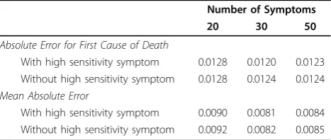
We first generate a“high sensitivity” symptom, which we shall study the effect of. It has 100% sensitivity for the first cause of death and 0% for predicting any other cause of death (i.e., it also has high specificity). (The prevalence of this first cause of death is 20% overall.) Every other symptom has a maximum of 30% sensitivity for any cause of death. For each of 20, 30, and 50 symp-toms, we generate 80 data sets with and without this high sensitivity symptom (each with 3,000 samples from the hospital and 3,000 from the community). In each data set, we estimate the CSMR. We then average over the 80 results for each combination of symptoms and compare the average of these estimates to the truth. This averaging is the standard way of setting aside the natural sampling variability and focusing on systematic patterns.
the effects for all causes of death. Again, the results show the irrelevance of including this high sensitivity symptom. (The numbers in the tables are proportions, so that 0.0128 represents a 1.28 percentage point differ-ence between the estimate and the truth.)
Searching for high sensitivity symptoms is thus at best a waste of time. The essential statistical reason for this is that symptoms do not cause the diseases and injuries that result in death. Instead, the symptoms are conse-quences of these diseases and injuries. As such, asses-sing whether the symptoms have high sensitivity and specificity for predicting something they do not predict (or cause) in the real world, and are not needed to pre-dict with the method, is indeed irrelevant.
The King-Lu method works by appropriately treating symptoms as consequences of the disease or injury that caused death. Even if they were available, having symp-toms that approximate highly predictive bioassays is neither necessary nor even very helpful. Any symptom which is a consequence of one or more of the causes of death can be used to improve CSMR estimates, even if it has random measurement error. So long as a symp-tom has some, possibly low-level, relationship to the causes of death, it can be productively used. Even appar-ently tertiary, behavioral, or non-medical symptoms that happen to be consequences of the illness can be used so long as they are likely to be reported in the same way regardless of whether the death occurred in a hospital or the community.
0.3 Detecting Biased Symptom Questions
Suppose we follow the advice offered on selecting symp-tom questions in Section 0.1, but we make a mistake and include a question which unbeknownst to us induces bias. An example would be a symptom which, for a given cause of death, is overreported in the hospi-tal vs the community. Appendix B shows that in some circumstances it’s possible to detect this biased symp-tom question, in which case we can remove it and rerun the analysis without the offending question. Since many
verbal autopsy instruments include a large number of questions, this procedure could be used to eliminate questions without much cost. In this section, we present analyses in simulated and real data that demonstrate the effectiveness of this simple procedure.
We thus conduct a simulations where different num-bers of symptom questions are“misreported” – that is, reported with different frequencies in the hospital and community samples for given causes of death. We gen-erate two sets of data, one with 3,000 deaths in each of the hospital and community samples and the other with 500 deaths in each; both have 10 different causes of death, with distributionD= (0.2, 0.2, 0.2, 0.1, 0.05, 0.05,
0.05, 0.05, 0.05, 0.05). The CSMF distribution ofD in
the hospital is uniform (0.1 for each cause) and in the community is D= (0.2, 0.2,..., 0.2, 0.05). Table 2 sum-marizes the pattern of misreporting we chose. In this table, the first row indicates which symptom number is to be set up as misreported when applicable. The sec-ond row gives the extent of the violation of the key
assumption of the King-Lu method (in Equation 3) –
the percentage point difference between the symptom’s marginal distribution in the community and hospital samples. For example, where three symptoms are misre-ported, we generate data using the first three columns of Table 2 and so the marginal prevalence of the first, fifth, and 10th symptoms in the community sample are set to be different from the hospital according to the first three elements of the second column. When five symptoms are misreported, the distribution of the first, fifth, 10th, 11th and 15th symptoms will be set to be dif-ferent in the degree as indicated, etc.
We first give our large sample and small sample results and then give a graphic illustration of the bias-efficiency trade-offs involved in symptom selection.
Larger Sample Size
For the large (n = 3, 000) simulation, Table 3
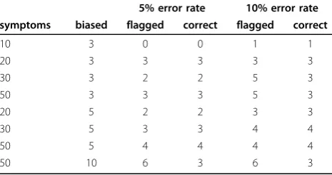
sum-marizes the results of symptom selection for each differ-ent simulation. The first two columns indicate, respectively, the total number of symptoms and the number of biased symptoms included in the community sample. The third column indicates the number of symptoms flagged (at the 5% significance level), using the selection procedure proposed in Appendix B. The final column indicates the number of biased symptoms that are correctly identified.
Table 3 indicates that our symptom selection proce-dure is highly accurate. Except the first simulation, which has disproportionately many misreported Table 1 Absolute error rates with and without a
symptom that has very high sensitivity for the first cause of death
Number of Symptoms
20 30 50
Absolute Error for First Cause of Death
With high sensitivity symptom 0.0128 0.0120 0.0123 Without high sensitivity symptom 0.0128 0.0124 0.0124 Mean Absolute Error
With high sensitivity symptom 0.0090 0.0081 0.0084 Without high sensitivity symptom 0.0092 0.0082 0.0085
The first and second row of each pair are very similar, which illustrates the irrelevance of finding symptoms with high sensitivity.
Table 2 List of Misreported Symptoms
Symptom 1 5 10 11 15 20 21 25 30 31
symptoms (three out of 10), our proposed method cor-rectly selects nearly all the biased symptoms. There is only one false positive case, but if we were to change the joint significance level to 0.01, this symptom would no longer being incorrectly selected.
Smaller Sample Size
Our smaller (n= 500) simulation necessarily results in larger CSMR variances. This, in turn, affects the power of the method described in Appendix B to detect biased symptoms. And at the same time it makes it more costly to discard unbiased symptoms. As shown in Table 4, we miss some symptoms at the 5% level. If we relax the type I error rate to 10%, more biased symptoms are detected. The table also conveys the additional variation in our methods due to the smaller sample size.
Bias-Efficiency Trade-offs
Although these results are encouraging, in real-world data, a trade-off always exists between choosing a lower significance level to ensure that all biased symptoms are selected at a cost of increasing the false positive rate, vs. choosing a higher significance level to reduce the false positive rate at the cost of missing some biased symp-toms. In this section, we illustrate how different sample sizes can affect the decision about the significance level in practice.
We now choose“large” (3, 000),“medium” (1, 000),
and “small” (500) samples for each of the community
and hospital samples. In each, 10 of 50 symptoms are biased. We then successively remove symptoms all the way up to the 50% signficance level criterion (to see the full consequence of dropping too many symptoms). Figure 1 gives the results in a graph for each sample size separately, (large, medium, and small sample sizes from left to right). Each graph then displays the mean square error (MSE) between the true and estimated cause-of-death distribution for each run of the model vertically, removing more and more symptoms as from the left to the right along the horizontal axis of each graph. (In real applications, we would never be able to compute the MSE, because we do not observe the true cause of death, but we can do it here for validation because the data are simulated.) That is, all symptoms are included for the first point on the left, and each subsequent point represents a model estimated with an additional symptom dropped, as selected by our proce-dure. Circles are plotted for models where a biased symptom was selected and solid disks are plotted for unbiased symptoms.
Three key results can be seen in this figure. First, for all three sample sizes and corresponding graphs, all biased symptoms are selected before any unbiased symptoms are selected, without a single false positive (which can be seen because all circles appear to the left of all solid disks).
Second, all three figures are distinctly U-shaped. The reason can be seen beginning at the left of each graph with a sample that includes biased symptoms. As our selection procedure detects and deletes these biased symptoms one at a time, the MSE drops due to the reduction in bias of the estimate of the CSMR. Drop-ping additional symptoms after all biased ones are dropped, which can occur if the wrong significance level is chosen, will induce no bias in our results but can reduce efficiency. If few unbiased symptoms are deleted, little harm is done since most verbal autopsy data sets have many symptoms and so enough efficiency to cover the loss. However, if many more unbiased symptoms are dropped, the MSE starts to increase because of ineffi-ciency, which explains the rest of the U-shape.
Finally, in addition to choosing the order in which symptoms should be dropped, our automated selection procedure also suggests a stopping rule based on the user-choice of a significance level. The 5% and 10% sig-nificance level stopping rules appear on the graphs as solid and dashed lines. These do not appear exactly at the bottom of the U-shape, cleanly distinguishing biased from unbiased symptoms, but for all three sample sizes the results are very good. In all cases, using this stop-ping rule would greatly improve the MSE of the ulti-mate estimator. Our procedure thus seems to do work reasonably well.
Table 3 Performance of the Symptom Selection Method withn= 3, 000
symptoms biased flagged correct
10 3 0 0
20 3 3 3
30 3 3 3
50 3 3 3
20 5 5 5
30 5 5 5
50 5 6 5
50 10 10 10
Table 4 Performance of the Symptom Selection Method withn= 500
5% error rate 10% error rate symptoms biased flagged correct flagged correct
10 3 0 0 1 1
20 3 3 3 3 3
30 3 2 2 5 3
50 3 3 3 5 3
20 5 2 2 3 3
30 5 3 3 4 4
50 5 4 4 4 4
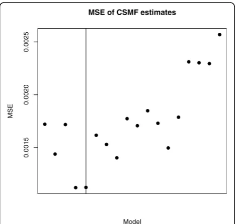
Empirical Evidence from Tanzania
Finally, we apply the proposed validation method to a real data example where we happen to observe the true causes of death in both samples [19]. These data from Tanzania have 12 causes of death and 51 symptoms questions but a small sample of only 282 deaths in the community sample and 1,261 in the hospital. Applying our symptom selection method, at the 5% level, four symptoms would be deleted, which in fact corresponds to the smallest MSE along the iterative model selection process. Figure 2 gives these results.
To illustrate this example in more details, Table 5 shows how the mean square error changes when specific symp-toms were sequentially selected, And in Table 6 we present
the change in each cause-specific mortality fraction esti-mate as these four symptoms are sequentially removed.
The first three symptoms which were sequentially dropped–fever, pale, and confused–are so non-speci-fic that they were almost unable to distinguish all of the 12 causes clinically, with the possible exception of deaths from injuries. Although high levels of specificity are not necessary for our method, we do require that it is above zero. Wheezing is a distinctive clinical symp-tom of an airway obstruction, typically observed in patients with asthma or bronchitis, and would be useful to identify deaths from such causes. However, our method suggests that it was highly biased. In fact,
Figure 1For sample sizes of 3,000 (left graph), 1,000 (middle), and 500 (right), the figure gives the mean square error as symptoms are removed using our detection diagnostic. The mean square error first declines, as bad symptoms are removed and bias drops, and then increases, as unbiased symptoms are dropped and variance increases. The procedure selects all biased symptoms (open circles) before unbiased symptoms (solid disks). The vertical line indicates where our automated procedure would indicate that we should stop.
Figure 2Validation of Mean Square Error in Tanzania, where the true cause of death is known in both samples.
Table 5 List of symptoms that are sequentially removed from the analysis
prevalence
symptoms hospital community mean square error
- - - 0.0016
fever 72.6 45.4 0.0013
pale 33.1 17.4 0.0018
confused 30.8 14.5 0.0012
wheezing 8.3 21.3 0.0012
vomit 49.0 35.5 0.0015
difficult-swallow 18.9 7.4 0.0015
diarrhoea 29.8 20.9 0.0014
chest-pain 43.9 33.0 0.0017
pins-feet 14.6 8.5 0.0015
many-urine 8.4 5.3 0.0016
breathless-flat 28.2 35.5 0.0015
pain-swallow 15.5 6.7 0.0015
mouth-sores 22.7 13.8 0.0018
cough 50.0 38.7 0.0020
body-stiffness 6.9 2.5 0.0021
puffiness-face 11.7 11.3 0.0025
Table 5 indicates that there was a substantial difference in the prevalence of wheezing between community and hospital deaths (8.3% and 21.3%, respectively). This would mean that the wheezing observed in the commu-nity may be highly biased due to the respondents’ diffi-culty in understanding the symptom correctly. Other symptoms which can be considered unbiased, such as vomiting, difficulty in swallowing, and chest pain, are all clinically useful in distinguishing the 12 causes of death, and the difference in prevalence between community and hospital deaths was much smaller.
0.4 Adjusting for Sample Differences
Suppose the key assumption of the King-Lu method is violated because of known differences in the hospital and community samples. For example, it may be that through outreach efforts of hospital personnel, or because of sampling choices of the investigators, chil-dren are overrepresented in the hospital sample. Even if the key assumption applies within each age group, dis-eases will present differently on average in the two sam-ples because of the different age compositions. When it is not feasible to avoid this problem by desiging a proper sampling strategy, we can still adjust ex post to avoid bias, assuming the sample is large enough. The procedure is to estimate the distribution of symptoms for each cause of death within each age group sepa-rately, instead of once overall, and then to weight the results by the age distribution in the community.
As Appendix A shows in more detail, this procedure can also be applied to any other variables with known distributions in the community, such as sex or educa-tion. Since variables like these are routinely collected in verbal autopsy interviews, this adjustment should be easy and inexpensive, and can be powerful.
Reducing Inefficiencies
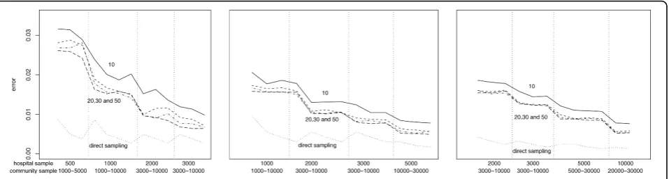
We now suppose that the analyst has chosen symptom questions as best as possible to minimize bias, and study what can be done to improve statistical efficiency. Effi-ciency translates directly into our uncertainty estimates about the CSMR, such as the standard error or confi-dence interval, and improving efficiency translates directly into research costs saved. We study efficiency by simulating a large number of data sets from a fixed population and measure how much estimates vary. We then study how efficiency responds to changes in the number of symptom questions (10, 20, 30, and 50), size of the hospital sample (500, 1,000, 2,000, 3,000, and 5,000), size of the community sample (1,000, 2,000, 3,000, 5,000, and 10,000), and number of chosen causes of death (5, 10, and 15). Causes of death in the hospital are assumed to be constructed via a case-control meth-ods, with uniform CSMR across causes. The CSMR in the community for each cause of death has some preva-lent causes and some rarer causes.
For each combination of symptoms, hospital and com-munity samples, and number of causes of death, we ran-domly draw 80 data sets. For each, we compute the absolute error between the King-Lu estimate and the truth per cause of death, and finally average over the 80
simulations. This mean absolute errorappears on the
vertical axis of the three graphs (for 5, 10, and 15 causes of death reading from left to right) in Figure 3. The hor-izontal axis codes both the hospital sample size and, within categories of hospital sample size, the community sample size. Each of the top four lines represent differ-ent numbers of symptoms.
The lower line, labeled “direct sampling,” is based on an infeasible baseline estimator, where the cause of each randomly sampled community death is directly ascer-tained and the results are tabulated. The error for this direct sampling approach is solely due to sampling variability and so serves as a useful lower error bound to our method, which includes both sampling variability and error due to extrapolation between the hospital and population samples. No method with the same amount of available information could ever be expected to do better than this baseline.
Figure 3 illustrates five key results. First, the mean abso-lute error of the King-Lu method is never very large. Even in the top left corner of the figures, with 500 deaths in the hospital, 1,000 in the community, and only 10 symptom Table 6 Cause-specific mortality fraction estimates when
the first four symptoms are removed
sequentially removed cause of
death
all 51 symptoms
fever pale confused wheezing true
HIV 0.146 0.177 0.164 0.185 0.190 0.227 Malaria 0.073 0.082 0.084 0.091 0.101 0.089 Tuberculosis 0.063 0.071 0.086 0.073 0.077 0.035 Infectious
diseases
0.058 0.047 0.050 0.044 0.044 0.028
Circulatory diseases
0.225 0.215 0.159 0.163 0.160 0.163
Maternal diseases
0.035 0.026 0.030 0.033 0.032 0.035
Cancer 0.042 0.033 0.033 0.039 0.041 0.092 Respiratory
diseases
0.070 0.079 0.070 0.073 0.053 0.046
Injuries 0.039 0.034 0.028 0.023 0.031 0.050 Diabetes 0.113 0.108 0.150 0.133 0.139 0.053 Other
diseases I*
0.023 0.031 0.030 0.027 0.027 0.032
Other diseases II
0.170 0.164 0.173 0.159 0.162 0.149
questions, the average absolute error in the cause-of-death categories is only about 2 percentage points, and of this 0.86, of a percentage point is due to pure irreducible sam-pling variability (see the direct samsam-pling line).
Second, increasing the number of symptom questions, regardless of the hospital and community sample sizes, reduces the mean absolute error. So more questions are better. However, the advantage in asking more than about 20 questions is fairly minor. Asking five times more questions (going from 10 to 50) reduces the mean absolute error only by between 15% and 50%. Our simu-lation is using symptom questions that are statistically independent, and so more questions would be needed if different symptoms are closely related; however, addi-tional benefit from more symptoms would remain small. Third, the mean absolute error drops with the number of deaths observed in the community, and can be seen for each panel separated by vertical dotted lines in each graph. Within each panel, the slope of each line drops at first and then continues to drop but at a slower rate. This pattern reflects the diminishing returns of collect-ing more community observations, so increascollect-ing from 5,000 to 10,000 deaths does not help as much as increasing the sample size from 1,000 to 3,000.
Fourth, mean absolute error is also reduced by increasing the hospital sample size. Assuming since data collection costs will usually keep the community sample larger than the hospital sample, increasing the hospital sample size will always help reduce bias. Moreover, within these constraints, the error reduction for collect-ing an extra hospital death is greater than that in the community. The reason for this is that the method esti-mates only the marginal distribution of symptom profile prevalences from the community data, whereas it esti-mates this distribution within each category of deaths in the hospital data. It is also true that the marginal gain in the community sample is constrained to a degree by the sample size in the hospital; the reason is that combi-nations of symptoms in the community can only be ana-lyzed if examples of them are found in the hospital.
And finally, looking across the three graphs in Figure 3, we see that the mean absolute error per cause drops slightly or stays the same as we increase the number of causes of death. Of course, this also means that with more causes, the total error is increasing as the number of causes increase. This is as it should be because esti-mating more causes is a more difficult inferential task.
The results in this section provide detailed informa-tion on how to design verbal autopsy studies to reduce error. Researchers can now pick an acceptable threshold level for the mean absolute error rate (which will depend on the needs of their study and what they want to know) and then choose a set of values for the design features that meets this level. Since the figure indicates that different combinations of design features can pro-duce the same mean absolute error level, researchers have leeway to choose from among these based on con-venience and cost-effectiveness. For example, although the advantage of asking many more symptom questions is modest, it may be that in some areas extra time spent with a respondent is less costly than locating and travel-ing to another family for more interviews, in which case it may be more cost-effective to ask 50 or more symp-tom questions and instead reduce the number of inter-views. Figure 3 provides many other possibilities for optimizing scarce resources.
Discussion
Despite some earlier attempts at promoting standard tools [20], which have now been adopted by various users including demographic surveillance sites under the INDEPTH Network [19,21,22], little consensus existed for some time on core verbal autopsy questions and methods. In order to derive a set of standards and to achieve a high degree of consistency and comparability across VA data sets, a recent WHO-led expert group recently systematically reviewed, debated, and condensed the accumulated experience and evidence from the most widely-used and validated procedures. This process resulted in somewhat more standardized tools, which
are now adopted by various users, including demo-graphic surveillance sites.
Verbal autopsy methodologies are still evolving: sev-eral key areas of active and important research remain. A research priority must be to carry out state-of-the-art validation studies of the new survey instruments in mul-tiple countries with varying mortality burden profiles, using the methods discussed and proposed here. Such a validation process would contribute to the other areas of research, including further optimization of items included in questionnaires; replicable and valid auto-mated methods for assigning causes of death from VA that remove human bias from the cause-of-death assign-ment process; and such important operational issues as sampling methods and sizes for implementing VA tools in research demographic surveillance sites, sample or sentinel registration, censuses, and household surveys.
With the advice we offer here for writing symptom questions, weeding out biased questions, and choosing appropriate hospital and community sample sizes, researchers should be able to greatly improve their ana-lyses, reducing bias and research costs. We encourage other researchers and practitioners to use these tools and methods, to refine them, and to develop others. With time, this guidance and experience ought to better inform the VA users, and enhance the quality, compar-ability, and consistency of causespecific mortality rates throughout the developing world.
Appendix A
The King-Lu Method and Extensions
We describe here the method of estimating the CSMR offered in [10]. We give some notation, the quantities of interest, a simple decomposition of the data, the estima-tion strategy, and a procedure for making individual classifications when useful.
Notation
Hospital deaths may be selected randomly, but the method also works without modification if they are selected via case-control methods whereby, for each cause, a fixed number of deaths are chosen. Case-con-trol selection can greatly increase the efficiency of data collection. Deaths in the community need to be chosen randomly or in some representative fashion. Define an index i (i = 1,...,n) for each death in a hospital and ℓ
(ℓ =1,..., L) for each death in the community. Then
define a set of mutually exclusive and exhaustive causes of death, 1,...,J, and denoteDℓas the observed cause for a death in the hospital andDias the unobserved cause
for a death in the community. The verbal autopsy
sur-vey instrument typically includes a set of Ksymptom
questions with dichotomous (0/1) responses, which we
summarize for each decedent in the hospital as aK× 1
vector Si = {Si1,...,SiK} and in the community as Sℓ=
{Sℓ1,...,SℓK}.
Quantity of Interest
For most public health purposes, primary interest lies not in the cause of any individual death in the commu-nity but rather the aggregate proportion of commucommu-nity deaths that fall into each category:P(D) = {P(D= 1),..., P(D=J)}, where P(D) is aJ× 1 vector and each element of which is a proportion: P D( = j)=1L
∑
L=11(D= j), where 1(a) = 1 if ais true and 0 otherwise. This is an important distinction because King-Lu gives approxi-mately unbiased estimates ofP(D) even if the percent of individual deaths correctly classified is very low. (We also describe below how to use this method to produce individual classifications, which may of course be of interest to clinicians.)Decomposition
For any death, the symptom questions contain 2K possi-ble responses, each of which we call a symptom profile. We stack up each of these profiles as the 2K × 1 vector
S and write P(S) as the probability of each profile
occurring (e.g., with K= 3 questionsP(S) would contain
the probabilities of each of these (23 = 8) patterns
occurring in the survey responses: 000, 001, 010, 011, 100, 101, 110, and 111). P(S|D) as the probability of each of the symptom profiles occurring within for a
given cause of death D(columns ofP(S|D)
correspond-ing to values ofD). Then, by the law of total probabil-ity, we write
P s P s D j P D j
j J
(S= )= (S= | = ) ( = ).
=
∑
1 (1)and, to simplify, we rewrite Equation 1 as an equiva-lent matrix expression:
P P P D
K K
J J
( )S (S ) ( ).
2 ×1 = 2 × ×1
| D (2)
whereP(D) is aJ× 1 vector of the proportion of com-munity deaths in each category, our quantity of interest. Equations 1 and 2 hold exactly, without approximations.
Estimation
To estimate P(D) in Equation 2, we only need to
esti-mate the other two factors and then solve algebraically.
We can estimateP(S) without modeling assumptions by
direct tabulation of deaths in the community (using the proportion of deaths observed to have each symptom profile). The key issue then is estimatingP(S|D), which is unobserved in the community. We do this by assum-ing it is the same as in the hospital sample,Ph(S|D):
This assumption is considerably less demanding than other data-derived methods, which require the full joint distribution of symptoms and death proportions to be the same:Ph(S, D) =P(S, D). In particular, if either the symptom profiles (how illnesses that lead to death pre-sent to caregivers) or the prevalence of the causes of
death differ between the hospital and community–Ph
(S) ≠P(S) or Ph(D) ≠ P(D)– then other dataderived methods will fail, but this method can still yield unbiased estimates. Of course, if Equation 3 is wrong, estimates from the King-Lu method can be biased, and so finding ways of validating it can be crucial, which is the motivation for the methods offered in the text. (Sev-eral technical estimation issues are also resolved in [10]: Because 2Kcan be very large, they use the fact that (2) also holds for subsets of symptoms to draw multiple random subsets, solve (2) in each, and average. They also solve (2) for P(D) by constrained least squares to ensure that the death proportions are constrained to the simplex.)
Adjusting for Known Differences Between Hospital and Community
Letabe an exogneous variable measured in both
sam-ples, such as age or sex. To adjust for differences in a between the two samples, we replace our usual estimate ofPh(S|D) with a weighted average of the same estima-tor applied within unique values of a,Ph(Sa|Da), times
the community distribution, f a Pa S D P D f a
h h
a
a a
( ) : ( | )=
∑
(S | ) ( ), and where the summation is over all possible values ofa.Individual Classification
Although the quantity of primary interest in verbal autopsy studies is the CSMR, researchers are often interested in classifications of some individual deaths. As shown in [[10], Section 8], this can be done with an application of Bayes theorem, if one makes an additional assumption not necessary for estimating the CSMR. Thus, if the goal is P(Dℓ=j|Sℓ=s), the probability that individualℓdied of causejgiven that he or she suffered from symptom profiles, we can calculate it by filling in the three quantities on the right side of this expression:
P D j P D j P D j
P
( | ) ( | ) ( )
( ) .
= = = = = =
=
S s S s
S s (4)
First is P(Dℓ=j), the optimal estimate of the CSMR, given by the basic King-Lu procedure. The quantity P(Sℓ=s|Dℓ=j) can be estimated from the training set, usually with the addition of a conditional independence
assumption, and P(Sℓ=sℓ) may be computed without
assumptions from the test set by direct tabulation. (Bayes theorem has also been used in this field for other creative purposes [23].)
A Reaggregation Estimator
A recent article [12] attempts to build on King-Lu by estimating the CSMR with a particular interpretation of Equation 4 to produce individual classifications which
they then reaggregate back into a “corrected” CSMR
estimate. Unfortunately, the proposed correction is in general biased, since it requires two unnecessary and substantively untenable statistical assumptions. First, it uses the conditional independence assumption for esti-matingP(Sℓ=s|Dℓ=j)–useful for individual classifica-tion but unnecessary for estimating the CSMR. And second, it estimates P(Sℓ=s) from the training set and so must assume that it is the same as that in the test set, an assumption which is verifiably false and unneces-sary since it can be computed directly from the test set without error [[10], Section 8]. To avoid the bias in this reaggregation procedure to estimate the CSMR, one can use the original King-Lu estimator described above. Reaggregation of appropriate individual classifications will reproduce the same aggregate estimates.
Appendix B
A Test for Detecting Biased Symptoms
If symptomk,Sk, is overreported in the community
rela-tive to the hospital for a given cause of death, then we
should expect the predicted prevalence P S
k
∧
( ) – which
can be produced by but is not needed in the King-Lu
procedure–to be lower than the observed prevalence P
(Sk). Thus, we can view P(Sk) as data point in regression
analysis and the misreported prevalence of the kth
symptom, P(Sk) as an outlier. This means that we can
detect symptoms that might bias the analysis by examin-ing model fit. We describe this procedure here and then give evidence and examples.
Test Procedure
Let P D∧( ) be the estimated community CSMRs via the
King-Lu procedure, and then fit the marginal prevalence
of the kth symptom in the community P S
k
∧
( )
(calcu-lated as P Sk Ph Sk Dj P Dj
j
∧ ∧
=
∑
( ) ( | ) ( ); see Appendix
A). Then define the prediction error as the residual in a
regression as e P S P S
k≡ k − k
∧
( ) ( ).
Under King-Lu, P D∧( ) is unbiased, and each ek is
mean 0 with variance V e ek e K
k K
( )=
∑
= ( − ) / (2 − )1 1 .
Moreover,
t ek e
ek e K
k = −
−
∑( ) /2 −1
is approximatelytdistributed withK- 1 degree free-dom. If, on the other hand,Ph(S|D)≠P(S|D), we would expecttkwill have an expected value that deviates from
Based on above observation, we propose a simple iterative symptom selection procedure. This procedure
avoids the classic the “multiple testing problem” by
applying a Bonferroni adjustment to symptom selection at each iteration. At the chosen significance levela, we can then assess whether a calculated value oftkindicates
that the kthsymptom violates our key assumption and
so is biased. Thus:
1. Begin with the set of all symptoms S= (S1,..., SK),
and those to be deleted, B. Initialize B as the null set, and the number of symptoms in the estimation, K0, asK0 =K.
2. EstimateP(D) using the King-Lu method.
3. For symptom k(k= 1,...,K0), estimate P S
k
∧
( ), and
calculatetk.
4. Find the critical value associated with level a
under the t distribution with K0 - 1 degree
free-dom, C[ /(#( ) B+1)],(K0−1). To ensure that the overall
significance of the all symptoms that belong to B
is less than a, use the Bonferroni adjustment for
the significance level (the set of tk test statistics
associated with the symptoms in set Bare
stochas-tically independent of each other since the models are run sequentially). The number of the multiple independent tests is counted as the number of
ele-ments already in the set B plus the one that is
being tested. (Since the maximum |tk| at each step
of symptom selection tends to decrease as more
“bad” symptoms are removed, it is sufficient to
check whether the maximum |tk| of the current
model is greater or less than the critical value,
C/(#( )B+1),(K0−1).)
5. If the largest value of |tk|, namely |tk’|, is greater than the critical value C[ /(#( ) B+1)],K0−1, remove the
correspondingk′ th symptom. Then setK0 =K0 - 1
and add symptomk′to setB.
6. Repeat step 2-5 until no new symptoms are
moved from StoB.
Acknowledgements
Open source software that implements all the methods described herein is available at http://gking.harvard.edu/va. Our thanks to Alan Lopez and Shanon Peter for data access. The Tanzania data was provided by the University of Newcastle upon Tyne (UK) as an output of the Adult Morbidity and Mortality Project (AMMP). AMMP was a project of the Tanzanian Ministry of Health, funded by the UK Department for International Development (DFID), and implemented in partnership with the University of Newcastle upon Tyne. Additional funding for the preparation of the data was provided through MEASURE Evaluation, Phase 2, a USAID Cooperative Agreement (GPO-A-00-03-00003-00) implemented by the Carolina Population Center, University of North Carolina at Chapel Hill. This publication was also supported by Grant P10462-109/9903GLOB-2, The Global Burden of Disease 2000 in Aging Populations (P01 AG17625-01), from the United States National Institutes of Health (NIH) National Institute on Aging (NIA) and from the National Science Foundation (SES-0318275, IIS-9874747, DMS-0631652).
Author details
1Institute for Quantitative Social Science, Harvard University, Cambridge MA
02138, USA.2Department of Humanities and Social Sciences in the Professions, Steinhardt School of Culture, Education and Human Development, New York University, USA.3Department of Global Health
Policy, Graduate School of Medicine, University of Tokyo, Japan.
Authors’contributions
GK, YL, and KS participated in the conception and design of the study and analysis of the results. YL wrote the computer code and developed the statistical test and simulations; GK drafted the paper. All authors read, contributed to, and approved the final manuscript.
Competing interests
The authors declare that they have no competing interests.
Received: 8 January 2010 Accepted: 23 June 2010 Published: 23 June 2010
References
1. Mathers CD, Fat DM, Inoue M, Rao C, Lopez A:Counting the dead and what they died from: an assessment of the global status of cause of death data.Bulletin of the World Health Organization2005,83:171-177. 2. Lopez A, Ahmed O, Guillot M, Ferguson B, Salomon J,et al:World
Mortality in 2000: Life Tables for 191 Countries.Geneva: World Health Organization 2000.
3. Sibai A, Fletcher A, Hills M, Campbell O:Non-communicable disease mortality rates using the verbal autopsy in a cohort of middle aged and older populations in beirut during wartime, 1983-93.Journal of Epidemiology and Community Health2001,55:271-276.
4. Setel PW, Sankoh O, Velkoff V, Mathers CYG,et al:Sample registration of vital events with verbal autopsy: a renewed commitment to measuring and monitoring vital statistics.Bulletin of the World Health Organization 2005,83:611-617.
5. Soleman N, Chandramohan D, Shibuya K:WHO Technical Consultation on Verbal Autopsy Tools.Geneva2005 [http://www.who.int/healthinfo/ statistics/mort verbalautopsy.pdf].
6. Thatte N, Kalter HD, Baqui AH, Williams EM, Darmstadt GL:Ascertaining causes of neonatal deaths using verbal autopsy: current methods and challenges.Journal of Perinatology2008, 1-8.
7. Anker M:Investigating Cause of Death During an Outbreak of Ebola Virus Haemorrhagic Fever: Draft Verbal Autopsy Instrument.Geneva: World Health Organization 2003.
8. Pacque-Margolis S, Pacque M, Dukuly Z, Boateng J, Taylor HR:Application of the verbal autopsy during a clinical trial.Social Science Medicine1990, 31:585-591.
9. Soleman N, Chandramohan D, Shibuya K:Verbal autopsy: current practices and challenges.Bulletin of the World Health Organization2006, 84:239-245.
10. King G, Lu Y:Verbal autopsy methods with multiple causes of death. Statistical Science2008,23:78-91 [http://gking.harvard.edu/files/abs/vamc-abs.shtml].
11. Todd J, Francisco AD, O’Dempsey T, Greenwood B:The limitations of verbal autopsy in a malaria-endemic region.Annals of Tropical Paediatrics 1994,14:31-36.
12. Murray CJ, Lopez AD, Feean DM, Peter ST, Yang G:Validation of the symptom pattern method for analyzing verbal autopsy data.PLOS Medicine2007,4:1739-1753.
13. Chandramohan D, Rodriques LC, Maude GH, Hayes R:The validy of verbal autopsies for assessing the causes of institutional maternal death. Studies in Family Planning1998,29:414-422.
14. Coldham C, Ross D, Quigley M, Segura Z, Chandramohan D:Prospective validation of a standardized questionnaire for estimating childhood mortality and morbidity due to pneumonia and diarrhoea.Tropical Medicine & International Health2000,5:134-144.
15. Quigley M, Schellenberg JA, Snow R:Algorithms for verbal autopsies: a validation study in kenyan children.Bulletin of the World Health Organization1996,74:147-154.
17. Kalter H:The validation of interviews for estimating morbidity.Health Policy and Planning1992,7:30-39.
18. Levy P, Kass EH:A three population model for sequential screening for bacteriuria.American Journal of Epidemiology1970,91:148-154. 19. Setel P, Rao C, Hemed Y, Whiting DYG,et al:Core verbal autopsy
procedures with comparative validation results from two countries.PLoS Medicine2006,3:e268, Doi:10.1371/journal.pmed.0030268.
20. World Health Organization:Verbal Autopsy Standards: Ascertaining and Attributing Causes of Death.Geneva: World Health Organization 2007. 21. Anker M, Black RE, Coldham C, Kalter HD, Quigley MA,et al:A standard
verbal autopsy method for investigating causes of death in infants and children.World Health Organization, Department of communicable Disease Surveillance and Response1999.
22. INDEPTH Network:Standardised verbal autopsy questionnaire2003 [http:// indepth-network.org].
23. Byass P, Fottrell E, Huong DL, Berhane Y, Corrah T,et al:(34) Refining a probabilistic model for interpreting verbal autopsy data, volume 2006. Scandinavian Journal of Public Health26-31.
doi:10.1186/1478-7954-8-19
Cite this article as:Kinget al.:Designing verbal autopsy studies. Population Health Metrics20108:19.
Submit your next manuscript to BioMed Central and take full advantage of:
• Convenient online submission
• Thorough peer review
• No space constraints or color figure charges
• Immediate publication on acceptance
• Inclusion in PubMed, CAS, Scopus and Google Scholar
• Research which is freely available for redistribution