Comparative quantification of health risks: Conceptual framework and methodological issues

Open Access

Review

Comparative quantification of health risks: Conceptual framework

and methodological issues

Christopher JL Murray

1

, Majid Ezzati*

2

, Alan D Lopez

3

, Anthony Rodgers

4

and Stephen Vander Hoorn

4

Address: 1_{Evidence and Information for Health Policy, World Health Organization, CH-1211 Geneva 27, Switzerland,} 2_{Risk, Resources and} Environmental Management Division, Resources for the Future, 1616 P Street NW, Washington DC 20036, USA, 3_{School of Population Health,} University of Queensland, Herston Road, Herston Qld 4006, Australia and 4_{Clinical Trials Research Unit (CTRU), University of Auckland, PB} 92019, Auckland, New Zealand

Email: Christopher JL Murray - [email protected]; Majid Ezzati* - [email protected]; Alan D Lopez - [email protected]; Anthony Rodgers - [email protected]; Stephen Vander Hoorn - [email protected] * Corresponding author

Abstract

Reliable and comparable analysis of risks to health is key for preventing disease and injury. Causal attribution of morbidity and mortality to risk factors has traditionally been conducted in the context of methodological traditions of individual risk factors, often in a limited number of settings, restricting comparability.

In this paper, we discuss the conceptual and methodological issues for quantifying the population health effects of individual or groups of risk factors in various levels of causality using knowledge from different scientific disciplines. The issues include: comparing the burden of disease due to the observed exposure distribution in a population with the burden from a hypothetical distribution or series of distributions, rather than a single reference level such as non-exposed; considering the multiple stages in the causal network of interactions among risk factor(s) and disease outcome to allow making inferences about some combinations of risk factors for which epidemiological studies have not been conducted, including the joint effects of multiple risk factors; calculating the health loss due to risk factor(s) as a time-indexed "stream" of disease burden due to a time-indexed "stream" of exposure, including consideration of discounting; and the sources of uncertainty.

Introduction

Detailed description of the level (e.g. rates) and distribu-tion of diseases and injuries, and their causes are impor-tant inputs to strategies for improving population health. Data on disease or injury outcomes alone, such as death or hospitalization, tend to focus on the need for palliative or curative services. Reliable and comparable analysis of risks to health, on the other hand, is key for preventing disease and injury. A substantial body of work has focused on the quantification of causes of mortality and more

re-cently burden of disease [1,2]. Analysis of morbidity and mortality due to risk factors, however, has frequently been conducted in the context of methodological traditions of individual risk factors and in a limited number of settings [3–10]. As a result, in most such estimates:

1) Causal attribution of morbidity and mortality to risk factors has been estimated relative to zero or some other constant level of population exposure. This single, con-stant baseline, although illustrating the total magnitude

Published: 14 April 2003

Population Health Metrics 2003, 1:1

Received: 20 February 2003 Accepted: 14 April 2003

This article is available from: http://www.pophealthmetrics.com/content/1/1/1

of the risk, does not provide visions of population health under other alternative exposure distribution scenarios. 2) Intermediate stages and interactions in the causal proc-ess have not been considered in the causal attribution cal-culations. As a result, attributable burden could be calculated only for those risk factor – disease combina-tions for which epidemiological studies had been con-ducted (often limited to individual risks).

3) Causal attribution has often taken place using exposure and/or outcome at one point in time or over an arbitrary period of time (for notable exceptions see the works of Manton and colleagues [11–13] and Robins [14–19]). Such "counting" of adverse events (such as death) has not been able to clearly distinguish between those cases that would not have occurred in the absence of the risk factor and those whose occurrence would have been delayed. More generally, this approach is unable to consider the ac-cumulated effects of time-varying exposure to a risk factor – in the form of years of life lost prematurely or lived with disability.

4) The outcome has been morbidity or mortality due to specific disease(s) without conversion to a comparable unit, making comparison among different diseases and/or risk factors difficult.

To allow assessing risk factors in a unified framework while acknowledging risk-factor specific characteristics, the Comparative Risk Assessment (CRA) module of the global burden of disease (GBD) 2000 study is a systematic evaluation of the changes in population health which would result from modifying the population distribution of exposure to a risk factor or a group of risk factors [20]. This unified framework for describing population expo-sure to risk factors and their consequences for population health is an important step in linking the growing interest in the causal determinants of health across a variety of public health disciplines from natural, physical, and med-ical sciences to the social sciences and humanities. In par-ticular, in the CRA framework:

1) The burden of disease due to the observed exposure dis-tribution in a population is compared with the burden from a hypothetical distribution or series of distributions, rather than a single reference level such as non-exposed. 2) Multiple stages in the causal network of interactions among risk factor(s) and disease outcome are considered to allow making inferences about combinations of risk factors for which epidemiological studies have not been conducted, including the joint effects of changes in multi-ple risk factors.

3) The health loss due to risk factor(s) is calculated as a time-indexed "stream" of disease burden due to a time-in-dexed "stream" of exposure.

4) The burden of disease and injury is converted into a summary measure of population health which allows comparing fatal and non-fatal outcomes, also taking into account severity and duration.

It is important to emphasize that risk assessment, as de-fined above, is distinct from intervention analysis, whose purpose is estimating the benefits of a given intervention or group of interventions in a specific population and time. Rather, risk assessment aims at mapping alternative population health scenarios with changes in distribution of exposure to risk factors over time, irrespective of wheth-er exposure change is achievable using existing intwheth-erven- interven-tions. Therefore, while intervention analysis is a valuable input into cost-effectiveness studies, risk assessment con-tributes to assessing research and policy options for reduc-ing disease burden by changreduc-ing population exposure to risk factors. Summary measures of population health (SMPH) and their use in the burden of disease analysis are discussed elsewhere [21,22]. The next three sections of this paper discuss the conceptual basis and methodologi-cal issues for the remaining three of the above points. We then discuss the sources and quantification of uncertainty.

Causal Attribution of Summary Measures of

Population Health to Risk Factors

used in attribution of diseases and injuries to occupation-al risk factors in occupationoccupation-al heoccupation-alth registries [8] and at-tribution of motor vehicle accidents to alcohol consumption. In general however, categorical attribution of SMPH to risk factors overlooks the fact that many dis-eases have multiple causes [26]. The epidemiological liter-ature has commonly used the counterfactual approach for the attribution of a SMPH to a risk factor, and compared mortality or disability under current distribution of expo-sure to the risk factor to those expected under an alterna-tive exposure scenario.

The dominant counterfactual exposure distribution in these studies has been zero exposure for the whole popu-lation (or a fixed non-zero level where zero is not possible such as the case of blood pressure when defined as pres-ence or abspres-ence of hypertension). The basic statistic ob-tained in this approach is the population attributable fraction (PAF) defined as the proportional reduction in disease or death that would occur if exposure to the risk factor were reduced to zero, ceteris paribus [27–35]. As dis-cussed by Greenland and Robins [36], attributable frac-tions without a time dimension are not able to characterize those cases whose occurrence would have been delayed in the absence of exposure. The authors rec-ommend the use of etiologic fractions with a time dimen-sion to account for this shortcoming. Time-based measures are discussed in more detail below.

The attributable mortality, incidence, or burden of disease due to the risk factor, AB, is then given as AB = PAF × B

where B is the total burden of disease from a specific cause or group of causes affected by the risk factor with a relative risk of RR.

The exposed population may itself be divided into multi-ple categories based on level or length of exposure each with its own relative risk. With multiple (n) exposure cat-egories, the PAF is given by the following generalized form:

Although choosing zero as the reference exposure may be useful for some purposes, it is a restricting assumption for

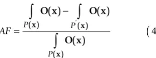
others. The contribution of a risk factor to disease or death can alternatively be estimated by comparing the burden due to the observed exposure distribution in a population with that from another distribution (rather than a single reference level such as non-exposed) as described by the generalized "potential impact fraction" in Equation 2 [32,37,38].

where RR(x) is the relative risk at exposure level x, P(x) is the population distribution of exposure, P' (x) is the coun-terfactual distribution of exposure, and m the maximum exposure level. The first and second terms in the numera-tor of Equation (2a) therefore represent the total expo-sure-weighted risk of mortality or disease in the population under current and counterfactual exposure distributions. The corresponding relationship when expo-sure is described as a discrete variable with n levels is given by:

In addition to relaxing the assumption of no-exposure group as the reference, analysis based on a broader range of distributions has the advantage of allowing multiple comparisons with multiple counterfactual scenarios. Equation 2a can be further generalized to consider coun-terfactual relative risks (i.e. relative risk may depend on other risks, new technology, medical services, etc.). For ex-ample the relative risk of injuries as a result of alcohol consumption may depend on road conditions and traffic law enforcement. Similarly, people employed in the same occupation may have different risk of occupational inju-ries because of different safety measures. Therefore, a more general form of Equation 2a is given by:

PAF P RR

P RR = − − +

( )

1 1 1a

PAF P RR P RR i i i n i i i n = − − +

( )

∑

∑

RR x P x dx RR x P x dx

RR x P x dx

x m x m x m = − ′

( )

∫

∫

∫

P RR P RR

P RR

i i i i

i n i n i i i n = − ′

( )

∑

∑

∑

RR x P x dx RR x P x dx

RR x P x dx

Counterfactual exposure distributions

Various criteria may determine the choice of the counter-factual exposure distributions. Greenland [39] has dis-cussed some of the criteria for the choice of counterfactuals, arguing that the counterfactuals should be limited to operationalizable actions (e.g. anti-smoking campaigns) rather than the effects of removing the out-comes targeted by those actions (e.g. smoking cessation) because in practice, the implementation of counterfactu-als for one risk factor or disease, may affect other risks. The solution to Greenland's concern, however, is better ana-lytical techniques for estimating joint risk factor effects, rather than abandoning non-intervention-based counter-factuals which, as argued by Mathers et al. [23], is a limit-ing view. An understandlimit-ing of the contributions from risk factors and the benefits of their removal, even in the ab-sence of known interventions, can provide visions of pop-ulation health attributable to risk factors, and avoidable by their removal. This knowledge of risk factor effects can provide valuable input into public health policies and pri-orities, as well as research and development (R&D). Murray and Lopez [20] introduced one taxonomy of counterfactual exposure distributions which, in addition to identifying the size of risk, provides a mapping to poli-cy implementation. These categories include the exposure distributions corresponding to theoretical minimum risk,

plausible minimum risk, feasible minimum risk, and cost-ef-fective minimum risk. Theoretical minimum risk is the ex-posure distribution that would result in the lowest population risk, irrespective of whether currently attaina-ble in practice. Plausiattaina-ble minimum refers to a distribution which is imaginable and feasible is one that has been ob-served in some population. Finally, cost-effective mini-mum considers the cost of exposure reduction (through the set of cost-effective interventions) as an additional cri-terion for choosing the alternative exposure scenario. In addition to illustrating the total magnitude of disease burden due to a risk factor, theoretical minimum risk dis-tribution (or the current difference between theoretical and plausible or feasible risk levels) can guide R&D re-sources towards those risk factors for which the mecha-nisms of reduction (i.e. interventions) are currently underdeveloped. For example, if the reduction in the bur-den of disease due to improved medical injection safety is high and the methods for risk reduction are well-known so that plausible/feasible and theoretical minima are identical, then current policy may have to be focused on the implementation of such methods. On the other hand, if there are large differences between plausible/feasible and theoretical minima risk levels for blood lipids or body mass index (BMI) [40], then research on reduction meth-ods and their implementation should be encouraged. For this reason the total magnitude of the burden of disease

due to a risk factor, as illustrated by the theoretical mini-mum, provides a tool for considering alternative visions of population health and setting research and implemen-tation priorities.

Biological principles as well as considerations of equity would necessitate that, although the exposure distribu-tion for theoretical minimum risk may depend on age and sex, it should in general be independent of geographical region or population. Exceptions to this are however una-voidable. An example would be the case of alcohol con-sumption, which in limited quantities and certain patterns, has beneficial effects on cardiovascular mortali-ty, but is always harmful for other diseases such as cancers and accidents [41]. In this case, the composition of the causes of death as well as drinking patterns in a region would determine the theoretical minimum distribution. In a population where cardiovascular diseases are a dom-inant cause of mortality theoretical minimum may be non-zero with moderate drinking patterns, whereas in a population with binge drinking and large burden from in-juries the theoretical minimum would be zero. Feasible and cost-effective distributions, on the other hand, may vary across populations based on the current distribution of the burden of disease and the resources and institutions available for exposure reduction.

The above categories of counterfactual exposure distribu-tions are based on the burden of disease in the population as a whole. Counterfactual exposure distributions may also be considered based on other criteria. For example, a counterfactual distributions based on equity would be one in which the highest exposure group (or the group with highest burden of disease) would be shifted towards low exposure values. Further, such equitable counterfactu-al distributions for each risk factor may themselves be cat-egorized into theoretical (most equitable), plausible, feasible, and cost-effective as described above. Similarly, a counterfactual distribution which focuses on the most sensitive groups in the population is one that gives addi-tional weight to lowering the exposure of this group. Therefore, by permitting comparison of disease burden under multiple exposure distributions, based on a range of criteria – including, but not limited to, implementation and cost, equity, and research prioritization – relaxing the assumption of constant exposure base-line provides an ef-fective policy and planning tool.

Exposure distribution for theoretical minimum risk

1) Physiological risk factors: This group includes those fac-tors that are physiological attributes of humans, such as blood pressure or blood lipids, and at some levels result in increased risk. Since these factors are necessary to sus-tain life, their "exposure-response" relationship is J-shaped or U-J-shaped, and the theoretical minimum is non-zero. For such risk factors, the choice of the theoretical minimum needs to be based on empirical evidence from different scientific disciplines. For example, epidemiolog-ical research on blood pressure and cholesterol have illus-trated a monotonically increasing dose-response relationship for mortality even at low levels of these risk factors [43–46]. But, given the role of these factors in sus-taining life, this relationship must flatten and reverse at some level. In the blood pressure and cholesterol assess-ment, a theoretical minimum distribution with a mean of 115 mmHg for systolic blood pressure and 3.8 mmol/l for total cholesterol (each with a small standard deviation) were used [42]. This distribution corresponds to the low-est levels at which the dose-response relationship has been characterized in meta-analyses of cohort studies [43–46]. Further, these levels of blood pressure and cho-lesterol are consistent with levels seen in populations which have low cardiovascular disease, such as the Yanomamo Indians [47] and rural populations in China [48,49], Papua New Guinea [47,50], and Africa [51]. Al-though, meta-analyses of randomized clinical trials have indicated that blood pressure and cholesterol levels may be lowered substantially with no adverse effects [52,53], it is difficult to justify a theoretical minimum lower than those measured in population-based studies, since lower levels in individuals may be caused by factors such as pre-existing diseases. Inferences from evolutionary biology would also support the lower bound on the choice of op-timal distribution based on historical survival of popula-tions who are not substantially exposed to factors that raise blood pressure or cholesterol.

2) Behavioral risk factors: the exposure-response relation-ship for this group of risk factors may be monotonically increasing or J-shaped. For risk factors with a monotonic exposure-response relationship, such as smoking, the the-oretical minimum would be zero unless there are physical constraints that make zero risk unattainable. For example in the case of blood transfusion, there may be a lower bound on safety of blood supply process even using the best monitoring technology. With a J-shaped or U-shaped exposure-response relationship, the theoretical minimum would be the turning point of the exposure-response curve. An example of this is alcohol consumption in adult populations with high cardiovascular disease rates, since moderate consumption may result in reduction in coro-nary heart disease in some age groups [54]. With a J-shaped exposure-response curve, similar to physiological

risk factors, empirical evidence would have to be used to determine the theoretical minimum.

Finally, some behavioral risks are expressed as the absence of protective factors such as physical inactivity or low fruit and vegetable intake. In such cases, optimal exposure would be the level at which the benefits of these factors would no longer continue. With a monotonic exposure-response relationship or without detailed knowledge about a possible turning point, the theoretical minimum risk level would have to be chosen based on empirical ev-idence on the highest theoretically sustainable levels of in-take or exposure (for example a purely vegetarian diet or a very active life style).

3) Environmental risk factors: The toxicity of most of the en-vironmental risk factors are monotonically increasing functions of exposure (potentially with some threshold). Therefore, the theoretical minimum for this group would be the lowest physically achievable level of exposure, such as background particulate matter concentration due to dust.

4) Socioeconomic "risk factors": Socioeconomic status and factors – such as income (including levels and distribu-tion) and associated levels of poverty and inequality, edu-cation, the existence of social support networks, etc. – are important determinants of health, often through their ef-fects on other risk factors. The efef-fects of each of these fac-tors on health are, however, highly dependent on other socioeconomic variables as well as the policy context, in-cluding accessibility and effectiveness of health and wel-fare systems. For this reason, the theoretical minimum exposure distribution, even if meaningfully defined, is likely to change over time and space depending on a large number of other factors. With this heterogeneity of effects, the effects of socioeconomic variables are best assessed relative to counterfactual distributions defined based on policy and intervention options in specific times and set-tings, as discussed by Greenland [39].

Risk Quantification Models

use a combination of aggregate and structural modeling. At the extreme, a structural model would attempt to use chemical or physical principles as the unit of analysis and modeling. This would of course be currently impossible in studying any system that involves population health. Consider for example predicting the future population of a city or the future ambient concentration of a pollutant. An aggregate model would extrapolate the historical levels to predict future values. Even in this case the model may include some structural elements. For example, the model may use a specific functional form – linear, exponential, quadratic, or logarithmic – for extrapolation which in-volves an assumption about the underlying system. A structural model in the case of population prediction would consider the age structure of the population, fertil-ity (which itself may be modeled using data on education and family planning programs), public health variables, and rural-urban migration (which itself can be modeled using economic variables). In the case of air pollution, a structural model may consider demographic variables (themselves modeled as above), the structure of the econ-omy (manufacturing, agriculture, or service), the current manufacturing and transportation technology and effects of R&D on new technology, the demand for private vehi-cles, the price of energy, and the atmospheric chemistry of pollution. Once again, in both examples the models may include some aggregation of variables by using the histor-ical trends to predict the future values of individual varia-bles in the system, such as funding for family planning or technology R&D.

The comparative advantage of structural and aggregate models lies in the balance between theoretical precision and data requirement. Structural models offer the poten-tial for more robust predictions, especially when the un-derlying system is complex and highly sensitive to one or more of its components. In such cases, a shift in some of the system variables can introduce large changes in the outcome which may be missed by extrapolation (such as the discovery of antibiotics and infectious disease trends or the change in tuberculosis mortality after the HIV epi-demic). Aggregate models, on the other hand, require considerably less knowledge of the system components and the relationships among them. These models can therefore provide more reliable estimates when such in-formation is not available, especially when the system is not very sensitive to its inputs in time intervals that are in the order of the prediction time.

Models for estimation of risk factor outcomes

Using the above aggregate – structural taxonomy, it is also possible to classify models that are used to predict chang-es in death or disease as a rchang-esult of changchang-es in exposure to underlying risk factor(s). Murray and Lopez [20]

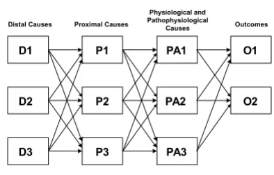
de-scribed a "causal-web" which includes the various distal (such as socioeconomic), proximal (behavioral or envi-ronmental), and physiological and patho-physiological causes of disease, in a structural model shown in Figure 1. While different disciplinary traditions, from social scienc-es and humanitiscienc-es, to physical, natural, and biomedical sciences have focused on individual components or stages of these relationships, in a single multi-layer causal model with interactions the term "risk factor" can be used for any of the causal determinants of health [23,55]. For example, poverty, location of housing, access to clean water and sanitation, and the existence of a specific parasite in water can all be considered the causes of diarrheal diseases, pro-viding a more complete framework for assessment of in-terventions and policy options. Similarly, education and occupation, diet, smoking, air pollution, and physical ac-tivity, and BMI and blood pressure are some of the risk factors at various levels of causality for cardiovascular diseases.

Compared to a causal-web, Equations 1 and 2 which use relative risk estimates from epidemiological methods such as Cox proportional hazard or other regression mod-els lie further towards aggregate modeling. In general, in such methods, relative risks are estimated so that they Figure 1

A causal-web illustrating various levels of disease causality. Feedbacks from outcomes to preceding layers may also exist. For example, individuals or societies may modify their risk behavior based on health outcomes. The "driving force, pres-sure, state, expopres-sure, effect" (DPSEE) model of Corvalan et al. [56] does consider the multiple layers of causality. These layers however focus the risk evolution process which is less suitable for multi-risk factor interaction within and between layers. More complete discussions of causality and multiple causes are provided by Yerushalmy and Palmer [55], Evans [57,58], and Rothman and Greenland [26,59].

D1

D2

D3

P1

P2

P3

PA1

PA2

PA3

O1

O2

Distal Causes Proximal Causes

Physiological and Pathophysiological

incorporate the aggregation of the various underlying re-lationship (ideally, but not always, controlling for the ap-propriate confounding variables) without considering intermediate relationships as separate causal stages (the exception is those risk factors whose effects occur through intermediate variables which are themselves a risk factor considered in the study, such as the relationships between CHD and physical inactivity or obesity which are mediat-ed through blood pressure or cholesterol. In such cases, controlling for the intermediate risk factor would result in a bias (towards the null) in the estimation of total hazard when the distal factor is considered alone [60]). On the other hand, if specified and estimated correctly, consider-ing the complete causal pathways which include multiple risk factors will allow making inferences about combina-tions of risk factors and risk factor levels for which direct epidemiological studies may not be available.

As discussed earlier, the appropriateness of the two ap-proaches to estimation of attributable burden depends on the specific risk factor(s), outcome, and available data. The relationship between smoking and lung cancer has been shown to be highly dependent on smoking patterns and duration which, with appropriate indicators of past smoking [3], can be readily estimated using the relative

risk approach of Equations 1 and 2. Consider, on the oth-er hand, the relationship among age, socioeconomic sta-tus and occupation, behavioral risk factors (such as smoking, alcohol consumption, diet, physical activity), physiological variables (such as blood pressure and cholesterol level), and coronary heart disease (CHD) shown in the causal diagram of Figure 2.

Given the multiple complex interactions, CHD risk may be best predicted using a structural (causal-web) ap-proach, especially when some risk factors vary simultane-ously, such as smoking, alcohol, and diet, requiring joint counterfactual distributions. Using a multi-risk model would also allow considering situations for which direct epidemiological studies may not have been conducted such as the effects of physical activity on those people who have diets different from the study group or those who use medicine to lower blood pressure.

The health effects of global climate change provide anoth-er example whanoth-ere a structural approach to risk assessment may be appropriate. Economic activity (including manu-facturing, agriculture and forest use, transportation, and domestic energy use) affect the emissions of greenhouse gases (GHG). Changes in precipitation, temperature or rainfall, and other meteorological variables due to atmos-pheric GHG accumulation alter regional ecology which in turn results in changes in agricultural productivity, quan-tity and quality of water, dynamics of disease vectors, and other determinants of disease. All these effects are in turn modulated by local economic activities, land-use patterns, and income [61–63]. A model based on the atmospheric physics/chemistry of GHG emissions and accumulation, climate models, plant and vector ecology, and human activity can provide a basis for the prediction of the health effects of climate change (there are no past studies on "cli-mate change" as it is expected to take place in the future. For this reason, the relationship between climate change and health would always be based on a model which re-lates climate change to meteorological variables (e.g. tem-perature or rainfall). The relationship between these variables, disease vectors and disease, could then be esti-mated from past data and vector biology [62,64,65]). Specifying the causal-web

Assuming for the moment no temporal dimension in the relationship between the different variables in the causal system (temporal aspects are discussed below), each layer of a causal-web may be characterized by the equation: Xn _{= ƒ(B(X}n-1_{, X}n_{), X}n-1_{) (3a)}

where Xn _{is the vector of the variables in the n}th _{layer of the} causal-web (which can be causal or output such as D, P, PA, or O using the notation of Figure 1); ƒ is the Figure 2

A possible causal diagram based on established relationships for estimating the incidence of coronary heart disease (CHD). Other interactions may also be possible.

CHD

Diabetes mellitus

LDL-Chol

DBP

Physical activity

Fat intake

BMI

Alcohol Age

Education

Income

functional form connecting the (n - 1)th _{layer to the n}th layer; B is a matrix of coefficients for ƒ which itself may be dependent on the variables in the (n - 1)th _{and n}th _layers (Xn-1 _{and X}n_{) (in this case when some of the variables}

af-fect not only the other variables in the causal system but also the relationship(s) between variables, they are equiv-alent to "effect modification" in epidemiological litera-ture [26]. Graphically, in Figure 1 they would be represented as links (arrows) not between two variables but as links from one of the variables (the effect modifier) to another link in the system), as well as time as we dis-cuss below.

If the variables in the nth layer of the causal-web are affect-ed directly by those in the (n-2)th _{layer in addition to the} (n-1)th _{layer, or by variables within the n}th _{layer itself (see} Figure 2 for an example), Equation 3a can be expanded to include these links as well:

Xn _{= ƒ(B}

0(Xn), Xn; B1 (Xn-1, Xn), Xn-1; B2(Xn-2, Xn), Xn-2) (3b)

This can be extended to interactions across multiple caus-al layers, and in genercaus-al any variable in the system can be affected by any other one as the concept of causal layer be-comes more flexible.

The attributable fraction of disease or mortality due to a single risk factor in the causal-web is then obtained by in-tegrating the outcome (O) over the current (P(x)) and counterfactual (P' (x)) population distributions of expo-sure, as was done in Equation 2.

Joint risk factor changes

The attributable fraction relationships described in Equa-tions 1 and 2 are based on individual risk factors. Disease and mortality are however often affected by multiple, and at times correlated, risk factors [26,38]. Estimating the joint effects of multiple distal and proximal risks is partic-ularly important because many factors act through other, intermediate, factors [20,55], or in combination with oth-er factors. It is thoth-erefore important to considoth-er how the burden of disease may change with simultaneous varia-tions in multiple risk factors. Considering joint risk factor changes implicitly indicates that the disease causation mechanism involves multiple factors, and is therefore suited to a causal-web framework, with P(x) and P' (x) in Equation 4 being the joint distributions of the vector of

risk factors, x. Alternatively, when using Equations 1 or 2, knowledge of the distribution of all relevant risk factors and the relative risk for each risk factor, estimated at the ap-propriate level of the remaining risk factors is required (in other words the RR(x) in Equations (2a) and (2b) are functions of the other covariates, which we referred to as effect modification earlier. Epidemiological studies that stratify relative risks based on covariates other than age and sex are however very rare). Therefore, in Equation 2a,

RR and P may represent joint risks and exposure distribu-tions for multiple risk factors [32]. In this case, the esti-mates from Equations 2a and 4 may in theory be identical.

Additivity of attributable fraction

Many users of risk assessment desire information charac-terized by additive decomposition. In other words, they would like to be able to answer what fraction of the dis-ease burden is related to any risk factor or group of risk factors, independent of the changes in other risk factors. As discussed by Mathers et al. [23], additive decomposi-tion is a property of categorical attribudecomposi-tion and, in general, not of counterfactual attribution because many diseases are caused by the interaction of multiple risk factors acting simultaneously and therefore can be avoided by eliminat-ing any of these factors [26,55,59]. Consider for example infant and child mortality due to acute respiratory infec-tions (ARI), which is especially high among malnourished children, as a result of exposure to indoor smoke from sol-id fuels [66,67]. In this case, removal of either risk factor will reduce mortality, some of which can therefore be at-tributed to both factors. Similarly the risk of mortality due to cardiovascular diseases among some of those who are affected by smoking, low physical activity, and poor diet may be reduced by elimination of any combination of these risk factors. Therefore, counterfactual causal attribu-tion of disease and injury to individual risk factors, does not normally allow additive decomposition and the sum of attributable fractions or burdens for a single disease due to multiple risk factors is theoretically unbounded. Although epidemiologically unavoidable and conceptual-ly acceptable, the lack of additivity presents additional policy complexity and implies great caution when com-municating and interpreting the estimates of attributable fraction and burden. With multiple attribution, the reduc-tion of one risk factor would seem to make other, equally important risk factors, potentially irrelevant from a per-spective with limited scope on quantification. At the same time multi-causality offers opportunities to tailor preven-tion based on availability and cost of intervenpreven-tions. It also necessitates the development of methods to quantify the effects of joint counterfactual distributions for multiple risk factors.

AF P P

P

=

−

( )

∫

∫

∫

O x O x

O x

x x

x

( ) ( )

( )

( ) ( )

( ) ’

Temporal Dimensions of Risk Factor – Disease

Relationship

Both exposure to a risk factor and the health outcomes due to exposure include a time dimension. This can be de-scribed by a modified version of Equation 3 in which ex-posure and outcome as well as the model parameters (B) are dependent on time. In the following two sections we consider the temporal characteristics of exposure and health outcomes.

Temporal characteristics of exposure

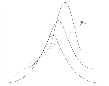
With the exception of acute hazards (e.g. injury risk fac-tors) exposure to a risk factor affects disease over a time period. As a result, the distributional transition between any two exposure distributions includes a temporal di-mension as illustrated schematically in Figure 3. The tran-sition path is of little importance if exposure changes over

a short time interval, especially relative to the time re-quired for the effect of exposure on disease. Over long time periods, however, there is sufficient time for contri-butions from the intermediate exposure values and the ac-tual path of transition may be as important as the initial and final distributions in determining the disease burden associated with change in exposure. For example, the ef-fects of reducing the prevalence of smoking or exposure to an occupational carcinogen by half in a population, would be markedly different if the change takes place im-mediately, gradually over a twenty-year period, or after twenty years. Therefore, the health effects of exposure to many risk factors depend on the complete profile of expo-sure over time, and may be further accompanied by a time-lag from the period of exposure. Also, for some risk factors there may be complete or partial reversibility, with the role of past exposure gradually declining.

Figure 3

A (three-dimensional) representation of a time-indexed distributional transition of population exposure to a risk factor, with a decreasing central tendency.

Exposure

% Population

To capture the effects of exposure profiles over time, we begin the analysis by considering the role of temporal di-mensions of exposure at the level of individuals (or groups of individuals with similar exposure) before ex-tending the analysis to the whole population. Suppose that at time T the relative risk of a disease, RR, for individ-uals exposed to a risk factor (compared to the non-ex-posed group) depends on the complete profile or stream of exposure between time T₀ and T, denoted by x(t), with some lag, L, between exposure and effect. Then, there is some function, ƒ(x), which can be used to describe the contribution of exposure at any point in time between T0 and T to the relative risk. In mathematical notation:

(The notation denotes "estimated between T₀ and

T").

The quantity is an equivalent exposure be-tween T₀ and T and is dependent on: 1) the profile of ex-posure (i.e. level of exex-posure at any point in time) described by x(t); and 2) the contribution of previous ex-posure to current hazard characterized by ƒ(x), an accumu-lative risk function. Note that equivalent exposure is an analytical concept and need not be physically realizable. In fact for many risk factors such as carcinogens where the effects are from life-long exposure, the equivalent expo-sure would be so high that its occurrence at a single in-stant would be impossible. Further, if there is threshold,

M, below which exposure has no effect:

where

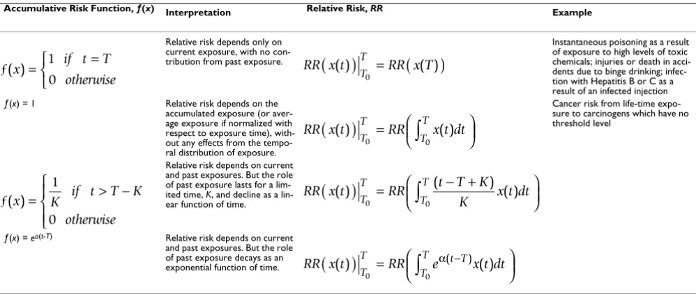
This framework can be easily modified to include cases where exposure has different effects below and above threshold by using TRUE(x(t) ≥M) for the effect above the threshold and TRUE(x(t) <M) for the effect below the threshold. Some potential forms for the accumulative risk function, ƒ(x), are given in Table 1.

The above framework can be extended from individuals to populations, by indexing the exposure profile (x(t)) to in-dividuals (i.e. representing the exposure of the ith individ-ual as xi(t)) and considering how the distribution of

exposure in the population evolves over time (in this manner, the evolution of the exposure distribution is analytically similar to a "random process" in which a probability density function (PDF) describes a random variable which is a function of time. Exposure to a risk fac-tor is not a random variable in the strict sense. But since a time-dependent exposure distribution has an accumulat-ed distribution of 1.0, it has the same representation as a random process). This in turn provides the population distributions of equivalent exposure (current or expected future and counterfactual) which form the basis of calcu-lating attributable fraction (i.e. the terms in the numerator or Equations (2a), (2b), or (4a)).

It is reasonable to assume that if the exposure of one indi-vidual is greater than that of another over the whole expo-sure period (i.e. tracking) [68], the equivalent exposure of the former is also greater than the latter. In other words, the accumulative risk function, ƒ(x), has the following property:

With this property, if the ordering of individuals in the ex-posure distribution remains unchanged over time (i.e. the rank-order correlation of individual exposures equals 1 between different points in time), the equivalent exposure will also have a distribution with the same ordering of individuals.

The method used by Peto et al. [3] for estimating mortality due to accumulated hazards of smoking implicitly uses such as framework. It is well-known that the accumulated hazards of smoking depend on a number of variables including the age at which smoking began, number of cig-arettes smoked per day, and cigarette type. Such data how-ever are extremely rare. To overcome this problem, Peto et al. [3] used smoking impact ratio, SIR, (which uses popu-lation lung cancer rates as a marker for accumulated haz-ard of smoking) to estimate the relative risk for the accumulated smoking exposure in the population. In the above notation:

The temporal profile of exposure for some risk factors may be more easily available than the range of indicators that

RR x t RR f x t L dt

T T

T T

( ) ( )

(

)

(

)



∫

( )

0 0

5

T T

0

ƒ x t( L dt) T

T

−

(

)

∫

RR x t RR x t L x t L M dt

T T

T T

( ) ( ) TRUE( ( ) )

( ) =  ( − ) ( − ≥ )



∫

0 0ƒ

TRUE( ( ) ) ( )

( )

x t M if x t M

if x t M

≥ = ≥

< 

  1 0

ƒ x t_i( ) dt ƒ x t( ) dt x t( ) x t( ) t T T, T

T

j T T

i j

( ) >

( )

[

]

∫

∫

6 if

RR smoking t RR smoking t L dt RR SIR T

T T

T T

( ) ( ) ( )

(

)

(

)



∫

(

)

are needed to estimate the accumulated hazards of smok-ing. For example, exposure to indoor smoke from solid fu-els is likely to remain unchanged as long as household fuel and housing conditions remain the same. Therefore, estimating the effects of long-term exposure may require only knowledge of household fuel, housing, and partici-pation in cooking. Similarly, in the case of blood pressure, it is known that blood pressure follows a predictable age-pattern [69,70], unless severely affected by a changes in social (stress), behavioral (diet or smoking), or medical circumstances. In this case, the usual blood pressure of an individual reflects the history of the person's exposure. On the other hand, the patterns of fruit and vegetable con-sumption, smoking, or exposure to ambient air pollution may change rapidly in countries with high rates of eco-nomic growth and urbanization, requiring more detailed data.

The above discussion is based on two implicit assumptions:

1) It considers the effects of exposure to a single risk factor over time. This approach may be appropriate for some risk factor – disease relationships (e.g. the effects of accumu-lated exposure to carcinogens with site-specific effects). But the single equivalent exposure cannot characterize other risk factor – disease relationships where risk factor interactions are important over time (e.g. physical activity, BMI, smoking and cardiovascular diseases). Extending

this temporal dimension to multiple risk factors requires considering the accumulated effects of the vector of risk factors as well as their interactions. In that case, Equation 5 would be expressed in terms the vector of risk factors of interest. Few epidemiological studies, however, have gath-ered the data needed for assessing accumulated interactive effects.

2) It considers exposure to each risk factor as an exoge-nous variable (i.e. intermediate exposure at any time, x(t), is not affected by disease or other risk factors) whose accu-mulated effect can be captured in single value using the risk accumulation function. For some risk factors, this as-sumption may not be valid since exposure to behavioral as well as environmental risk factors may be affected by knowledge of their current effects. Individuals may change their diet or activity levels based on knowledge of their weight or blood pressure and governments may in-troduce regulations based on the level of various contam-inants in air or water. Robins [18] discusses this issue in the case of estimating the effects of a dynamic treatment regime whose dose is dependent on symptoms.

Manton et al. [12,71] have relaxed these assumptions us-ing a diffusion model for forecastus-ing cardiovascular dis-ease mortality in the US. In this model, it is the change in the outcome in any time, t, that is modeled as a function of all the other variables in the system (i.e. other risk

fac-Table 1: Examples of accumulative risk functions

Accumulative Risk Function, ƒ(x) _{Interpretation} Relative Risk, RR _Example

Relative risk depends only on current exposure, with no con-tribution from past exposure.

Instantaneous poisoning as a result of exposure to high levels of toxic chemicals; injuries or death in acci-dents due to binge drinking; infec-tion with Hepatitis B or C as a result of an infected injection

ƒ(x) = 1 Relative risk depends on the

accumulated exposure (or aver-age exposure if normalized with respect to exposure time), with-out any effects from the tempo-ral distribution of exposure.

Cancer risk from life-time expo-sure to carcinogens which have no threshold level

Relative risk depends on current and past exposures. But the role of past exposure lasts for a lim-ited time, K, and decline as a lin-ear function of time.

ƒ(x) = ea(t-T) _{Relative risk depends on current}

and past exposures. But the role of past exposure decays as an exponential function of time.

For simplicity of notation, in all these cases we assume that: 1) L = 0. Including a lag is straightforward and can be done by replacing t with (t - L) in the corresponding formulas; and 2) there is no threshold for exposure. Including the threshold level is also straightforward using the TRUE (x (t) ≥

X) function. In scenarios 1, 3, and 4, where the effects of past exposure declines over time, risk reversibility can take place if exposure is reduced or removed. In 1 there is immediate risk reversibility; in 3, there is full reversibility after time K; in 4, risk reversibility asymptotically reaches 100%. In scenario 2 there is no risk reversibility and the effects of past exposure remain for an indefinite period.

ƒ( )x if t T

otherwise

=_ =

 1 0

RR x t RR x T

T T

( ) ( )

(

)

(

)

0

RR x t RR x t dt

T T

T T

( ) ( )

(

)



∫

0 0

ƒ( )x K if t T K

otherwise =_ > −

 1

0

RR x t RR t T K

K x t dt

T T

T T

( ) ( ) ( )

(

)



 

∫

0 0

RR x t RR e x t dt

T

T _{t T}

T T

( ) ( ) ( )

(

)



∫

0 0

tors as well as outcomes) and their interactions. Using the notation of Equation 3:

dX(t) = u(X(t), t) dt (7)

where u(X(t), t) is a drift term whose value depends on the current value of all the variables in the system as well as their interactions (and can be described by a functional form similar to that in Equation 3) (the diffusion model also includes a stochastic component to account for those interactive effects not described by the drift term). Meth-ods for estimation of such models using longitudinal data are discussed by Robins [19,72].

Temporal characteristics of health outcomes

If the outcome variable used in causal attribution of dis-ease and mortality to a risk factor only involves counting of adverse events (such as disease incidence or death), it is not possible to characterize those cases whose occurrence would have been delayed in the absence of the risk factor [16,36,73]. Therefore, this approach is unable to consider the accumulated effects of exposure – in the form of years of life lost prematurely or lived with disability. Parameterizing the above relationships by age (or birth cohort) would allow estimating the effects of exposure to a risk factor not as an event without time dimension but as an event at a certain age and time. More broadly con-sidering the time-indexed stream of health losses due to a risk factor requires using a time-based (and not event-based) SMPH.

Murray and Lopez [20] have provided an additional tem-poral distinction for the burden of disease due to a risk factor by introducing the concepts of "attributable" and "avoidable" burden. Attributable burden is defined as the reduction in the current or future burden of disease if the

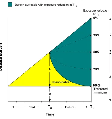
past exposure to a risk factor had been equal to some coun-terfactual distribution. Avoidable burden is the reduction in the future burden of disease if the current or future expo-sure to a risk factor are reduced to a counterfactual distri-bution. Attributable and avoidable burden are shown graphically in Figure 3. While attributable burden is easier to measure and more certain, avoidable burden is more useful for policy purposes. The distinction between attrib-utable and avoidable burden becomes less significant as the time between exposure to risk factor and effects on dis-ease burden decrdis-eases, which also makes attributable bur-den a better predictor of avoidable.

Figure 4 also illustrates a conceptual complexity in defin-ing and estimatdefin-ing avoidable burden. Attributable burden is defined based on the difference between (accumulated) current exposure and a counterfactual. Measuring current exposure, while difficult and uncertain, is conceptually well-defined. Avoidable burden, on the other hand,

de-pends on the expectation of future exposure and counter-factual, with the former being analogous to current exposure. Consider for example a population exposed to rising air pollution or obesity. In this setting, interven-tions that would maintain pollutant concentrainterven-tions or body mass index (BMI) at their current levels would result in avoiding disease and mortality; they reduce exposure compared to what it would be in their absence. Therefore, avoidable burden (i.e. how much of future burden can be prevented) by definition requires estimates of future expo-sure (i.e. how much of future burden there is). Projecting future exposure in turn raises the need to provide a projec-tion framework. To provide visions of public health under various intervention and policy scenarios we suggest the future exposure, with respect to which avoidable burden is estimated, to be the expectation of exposure if the cur-rent policy and technological context continued, referred to as "business-as-usual" (BAU) exposure trend. Therefore avoidable burden is the burden of disease averted due to reduction in exposure to a risk factor beyond its expected trends. We emphasize that with this definition, avoidable burden is the difference between two exposure scenarios: the expectation of future trends (BAU) and a reduction with respect to this trend towards theoretical minimum. Cumulative versus snap-shot estimates of attributable and avoidable burden

Although analytically inconsequential, the starting point and the duration of the time interval over which attribut-able or avoidattribut-able burden is reported has important policy implications because reductions in various risk factors may provide health benefits that occur after short or long delays and last for different durations. Consider for exam-ple the health benefits of reductions in binge alcohol con-sumption, smoking, and green house gas (GHG) emissions. Reducing binge drinking would result in im-mediate health benefits from a drop in alcohol related ac-cidents and injuries (as well as medium and long term benefits from reduction in other diseases). Lowering smoking will have some short and medium-term benefits from reduction of acute respiratory diseases and cardio-vascular disease as well as longer term benefits from low-ering cancers and chronic obstructive pulmonary disease (COPD). Finally, the benefits of policies that reduce cli-mate change as a result of GHG emissions are likely to be heavily concentrated in the future.

Figure 4

Attributable and avoidable burden. a = disease burden at T₀ attributable to prior exposure. The burden not attributable to risk factor of interest (light area) may be decreasing, constant, or increasing over time. The middle case is shown in the figure. b = disease burden at T₀ not attributable to the risk factor of interest (caused by other factors only). Dashed arrows represent the path of burden after a reduction at T₀. c = disease burden avoidable at T_x with a 50% exposure reduction at T₀. d = remaining disease burden at T_x after a 50% reduction in risk factor.

Burden not attributable to or avoidable with the risk factor of interest

Burden attributable to prior exposure

Burden avoidable with exposure reduction at T 0

Unavoidable

Disease Burden

Time

T

T

Past Future

0%

25%

50%

75%

100%

(Theoretical minimum)

c

d

a

b

large and important for the current cohort, the former pol-icies have one-time health benefits (unless repeated) while those of the latter are likely to last indefinitely. The above discussion would motivate reporting the esti-mates of avoidable burden in multiple ways including both snap-shots (for example annual) and cumulative es-timates as well as over short and long time frames. The is-sue of future estimates and their policy relevance is further complicated by the growing uncertainty in estimates with increasing the length of the estimation interval. Therefore, while it is ideal to increase the prediction horizon, it is im-portant to emphasize that long-term predictions are in-herently more uncertain.

Discounting future risk and health effects

Individuals may discount consumption or welfare within their own life span and exhibit a preference for benefits to-day over future. The theoretical and empirical arguments for and against individual discounting with specific em-phasis on health, including the possibility of negative dis-count rates, are summarized by Murray and Acharya [21,74] and are directly incorporated in calculating a sum-mary measure of population health. In addition to indi-vidual discounting and discount rates, policies dealing with risk confront the issue of addressing benefits to dif-ferent populations across time. As a result these policies must address ethical and analytical dilemmas related to the valuation of current and future health and welfare, in the form of social discount rates [75]. Discounting future risks, benefits, and welfare has been a subject of great de-bate [76–80], motivating some economists to conclude that "maybe the idea of a unitary decision-maker – like an optimizing individual or a wise and impartial adviser – is not very helpful when it comes to the choice of policies that will have distant-future effects about which one can now know hardly anything. Serious policy choice may then be a different animal, quite unlike individual saving and investment decisions. ... "Responsibility" suggests something less personal" [81].

The arguments for and against discounting of future health and welfare and their validity have been discussed in detail elsewhere [74,82–84]. According to one specific argument, "the disease eradication and health research paradox", not discounting future health would imply in-vesting all of society's health resources in research pro-grams or propro-grams for diseases eradication, which result in an infinite stream of benefits, rather than any programs that improve the health of the current generation. Such an excessive intergenerational "sacrifice" is a particularly powerful argument for discounting of future health (or more precisely for something that resembles discounting as we discuss shortly) [82]. It is important to emphasize that this argument does not claim that future welfare or

health is less valuable than current, but rather uses dis-counting as a tool to avoid excessive sacrifice to the cur-rent generation, to the point of investing all resources in an infinite stream of future health. For this reason, Parfit [82] argues that the issue of intergenerational distribution should be considered as an independent criterion, rather than in the form of discounting of future benefits. Koopmans [85], Dasgupta and Mäler [86], and Dasgupta

et al. [87], however, have shown that any preference-or-dering defined over the set of well-being paths over time can be represented by a numerical function with an appar-ently utilitarian form and therefore includes what resembles

positive discounting of future well-being (the functional

form is where 0 < α < 1 in [85] and

where δ > 0 in [86,87] α and δ are the social rate of dis-count). We emphasize that this notion is simply a conse-quence of considering the paths of well-being (or temporal distributions), rather than a statement on the value of current or future welfare. With this formulation, Dasgupta and Mäler [86] and Dasgupta et al. [87] consider the implications of the choice of discount rate as a "de-rived notion", as opposed to a value judgment. Dasgupta and Heal [88] and Solow [89] have shown that if well-be-ing is a result of consumption of an exhaustible resource, zero discount rate would imply investing all available re-sources for the benefit of future generations, and hence no current consumption. This is because each unit sacrificed by the first generation would yield a finite loss to this gen-eration, but an infinite stream of benefits to future gener-ations [90] which, without discounting, would always be larger than the one-time sacrifice. Although the first gen-eration cannot sacrifice everything (the last unit of sacrifice will have an infinite marginal utility therefore matching the future infinite stream of benefits), the logi-cal conclusion of this situation would be that "given any investment [for future benefits], short of the entire in-come, a still greater investment would be preferred," [90] or a potentially excessive intergenerational sacrifice [21]. On the other hand, a positive discount rate would imply that in the long run consumption of resources should be-come zero. In this case, however, the additional require-ment that well-being should never fall below a certain threshold would in turn require downward adjustment of the discount rate [91]. The stricter requirement of non-de-clining consumption and well-being would require a dis-count rate lower than the productivity of capital [86] (these two additional constraints are external to the eco-nomic efficiency arguments as defined by maximizing aggregate welfare. In fact, these additional constrains of minimum acceptable or non-declining welfare result in an "inefficient" outcome in order to achieve better

distri-W_tαt

0

∞

∫

∞

∫

0

bution across generations [92]; see Weitzman [93] for an-other argument for the choice of lower discount rates). Based on these arguments, we suggest discounting of fu-ture attributable or avoidable disease burden due to risk factors, but with a low discount rate, to include the wel-fares of both current and future generations as described above.

Uncertainty

Quantitative risk assessment is always affected by uncer-tainty about the existence, magnitude, and distribution of risk [94]. Quantitative analysis of uncertainty greatly adds to the applicability of the results because it shows not only the "best-estimate" magnitude and distribution of expo-sure to a risk factor and resulting burden of disease but also the range of potential outcomes.

Sources of uncertainty in attributable fractions

Population distribution of exposure

Due to complexity and cost, for most risk factors, expo-sure is meaexpo-sured only in small samples and in a limited number of settings. As we discussed earlier, because a risk factor can be represented in different layers of causality, variables for which data are more readily available can be used as exposure proxies. The use of exposure proxies is sometimes also necessary because epidemiological stud-ies have used such proxstud-ies in estimating hazard size. For example, anthropometric variables such as height-for-age or weight-for-age are used as indicators of childhood nu-tritional status, the presence of clean water sources or san-itary latrines as indicators of faecal-oral transmission of pathogens, concentration of particulate matter as the measure of exposure to the various pollutants in ambient air, and so on. In addition to reduced data requirements, the use of such indirect indicators of exposure (or expo-sure scenarios [95]) may provide direct mapping to exist-ing interventions. At the same time, these indicators, which are often more distal than actual exposure, do not capture the variability of exposure within each scenario, unless combined with other indicators which affect this variability [96]. For example people using the same water source may experience different levels of faecal-oral trans-mission of pathogens due to different storage behaviors. Therefore, the use of indirect exposure proxies results in additional uncertainty in exposure characterization. Even with the choice of exposure proxies, extrapolation of exposure between different populations or age groups is often necessary. Such extrapolation (or spatial prediction) can be based on models as simple as using the average of populations with data for a whole geographical region or more complex prediction models. For example, urban air quality monitoring systems provide data on particulate matter concentrations in some but not all cities in each re-gion. Models to predict ambient concentration based on

energy consumption, number of vehicles, and level of in-dustrialization can be used to predict ambient air pollu-tion levels for the cities where data are not available. Similarly, the level of physical (in)activity in a population may be predicted from a model that uses rural-urban pop-ulation distribution, income, education, distribution in occupational categories, and available transportation modes in each geographical region. Each such extrapola-tion adds to the uncertainty of exposure distribuextrapola-tions. Finally, as we discussed earlier, for many risk factors, haz-ards are associated with accumulated effects of sustained exposure. Indicators of accumulated hazard for those risk factors with changing exposure such as smoking, ambient urban air pollution, or body mass index, are needed but not always available. Further, few epidemiological studies have consider the role of temporal profile of exposure on disease (see Peto [97] for an example of an exception). Therefore even if longitudinal data on exposure preva-lence were available, they could not always be used to-gether with epidemiological studies that consider a single exposure variable, at the beginning or end of the follow-up period for example. At the same time, if the ordering of individuals in the exposure distribution remains un-changed over time (see above), risk estimates from epide-miological studies with similar ordering may be applicable, but results in an additional source of uncertainty. If exposure is sustained for a longer time in the risk assessment population than in the study popula-tion and if the whole exposure period contributes to haz-ards, this would result in an underestimation of risk (and vice versa). For example, in many cohorts in current epi-demiological studies, BMI increased when the subjects were in their twenties or thirties. There is however increas-ing child and adolescent overweight or obesity in many regions of the world. If this continues into adult life, the hazards may be higher than those subjects in the current study cohorts.

Risk factor – disease relationship

Par-asitology, and increasingly biophysics in establishing dis-ease causation.

Even when causality is established, the magnitude of the hazard due to a risk factor needs to be quantified. Al-though the statistical issues around establishing causality and estimating the effect size are similar (lack of causality is equivalent to zero excess risk) [18,100], in practice with knowledge from multiple disciplines in establishing cau-sality, it is often the latter that is the source of increased uncertainty in risk assessment. For example, the collectivity of scientific knowledge from disciplines such as economics and behavioral sciences, vector biology, physiology and bio-mechanics, and epidemiology would confirm the possibility that climate change or inequality would increase disease, or whether the relationships be-tween occupational factors or physical inactivity and low-er back pain are causal. At the same time, risk assessment would require estimating the hazard magnitude for each of these relationships. Therefore, the complexity of the causal relationship or lack of detailed data would shift the debate from causality to hazard size.

Epidemiological studies that quantify hazards are often conducted in a limited number of settings, with emphasis on estimating the average effect size in the whole study group. While the robustness of relative measures risk has been confirmed for more proximal factors in studies across populations [45,101], their extrapolation is an im-portant source of uncertainty for more distal risks (e.g. childhood sexual abuse) or those whose effects are heter-ogeneous (e.g. alcohol and injuries versus alcohol and cancer) and has received less attention in epidemiological literature [102]. At least for some risk factors, it is likely that the magnitude of hazard may depend on the levels of other variables (i.e. effect modifiers). Therefore in extrap-olating the results of individual epidemiological studies or meta-analyses, the very strength of the original study – applicability to the average person – would be the source of uncertainty if the population to whom the effect size is extrapolated has characteristics which would result in ef-fect modification [103–106]. The role of alcohol drinking patterns on cardiovascular disease risk estimates [41,107] are an example of the importance of considering the mod-ulating effects in risk extrapolation.

Risk factor and disease correlations

Because multiple risks and disease are correlated (e.g. higher malnutrition, unsafe water, sanitation, and hy-giene, indoor smoke and childhood mortality in poor ru-ral households in developing countries; higher smoking, BMI, and occupational risks in developed countries [108]), estimating attributable fractions would require stratified (e.g. by other risk factors) prevalence as well as disease data. Lack of stratified data is another source of

uncertainty, in general leading to underestimation of ef-fects in the presence of positive risk factor correlation [34].

Characterizing and quantifying uncertainty

Various taxonomies of uncertainty have been used in risk assessment [99] including:

1) classification based on information type such as uncer-tainty in hazard identification, exposure assessment, ex-posure-response assessment, as discussed above;

2) classification based on uncertainty type such as ran-domness, true variability, and bias; and

3) classification based on the approach to handling uncer-tainty which divides unceruncer-tainty into model uncertainty

and parameter uncertainty. Parameter uncertainty includes the uncertainty quantifiable using random-variable meth-ods such as uncertainty due to sampling and measure-ment error. Model uncertainty is due to gaps in scientific theory, measurement technology, and data [99]. It in-cludes uncertainty in the knowledge of causal relation-ships or of the form of the exposure-response relationship (threshold versus continuous, linear versus non-linear, etc.), the level of bias in measurement, etc. Defined broad-ly, model uncertainty also includes extrapolation of expo-sure or hazard from one population to another. Uncertainty in international risk assessment is by far dom-inated by model uncertainty, which is a result of lack and difficulty of direct studies on exposure, hazard, and back-ground disease burden.

es-timation and extrapolation of exposure-response relationships or relative risks that are measured in a limit-ed number of settings. In the presence of multiple esti-mates of hazard, it is common to use meta-analytical approaches to obtain an overall estimate. At the same time, the differences between various estimates may re-flect true variability in effect size, especially if obtained from different populations, resulting in uncertainty in hazard estimates.

Parameter uncertainty can be readily included in quanti-tative analysis using random-variable statistical tools [109]. While we have discussed the various sources of un-certainty, the important issue of extrapolation of exposure and hazard using models requires new approaches to quantifying uncertainty in the presence of limited data. Quantitative analysis of model uncertainty by definition would require considering the uncertainty of the models and assumptions used (including assumptions about dis-ease mechanism or data/parameter extrapolation) using tools of Bayesian statistics.

Conclusions

We have described a framework for systematic quantifica-tion of the burden of disease due to risk factors which at-tempts to unify the growing interest in health risks in a number of health, physical, and social sciences. We have discussed the following attributes of the framework along with the corresponding methodological issues that arise in its application:

1) comparing the burden of disease due to the observed exposure distribution in a population with the burden from a hypothetical distribution or series of distributions, rather than a single reference level such as non-exposed; 2) considering the multiple stages of causality and interac-tions between risk factor(s) and disease outcome to allow making inferences about combinations of risk factors for which epidemiological studies have not been conducted, including the joint effects of changes i