a I thank two anonymous referees and the editor for very insightful comments. I also thank Sophia Ding, Ugo Panizza, Janosch Weiss, Florian Egli, Wanlin Ren, Mark Hack, Michelle Cunningham, Sarah Haag, Elise Grieg, Etienne Michaud, and Martina Hengge for helpful comments. Lastly, I am very grateful to the Swiss Federal Statistical Office for providing the data.
b Department of International Economics, The Graduate Institute of International and Devel-opment Studies, Maison de la Paix (Chemin Eugène-Rigot 2), Case Postale 136, 1211 Geneva 21, Switzerland; KOF Swiss Economic Institute, ETH Zurich, Leonhardstr. 21, 8092 Zurich, Switzerland. Email: [email protected].
Christian Stettlerb
JEL-Classification: F14, F31, E52, Z31
Keywords: Real Exchange Rate, Tourism, Overnight Stays, Swiss Franc, Switzerland.
SUMMARY
1. Introduction
Fears of the Swiss tourism industry loom large since January 15, 2015. On this day the Swiss National Bank (SNB) removed the exchange rate floor of 1.20 Swiss francs per euro. Immediately after the announcement, the Swiss franc strongly appreciated against the euro and other major currencies. In the context of the ongoing debate on the consequences of the Swiss francs appreciation, this paper analyses the effect on the tourism industry of different Swiss communities by estimating the impact of a change in the real exchange rate on the number of overnight stays in Swiss hotels. Although the international literature on the topic is large, only few studies exist for Switzerland. Abrahamsen and Simmons-Süer (2011) analyse the impact of exchange rate movements on the number of over-night stays in Swiss hotels with data up to 2010. Falk (2014) estimates the effect of a change in the CHF/EUR exchange rate on Swiss alpine tourism. Ferro Luzzi and Flückiger (2003) and Jaeger, Minsch, and Abrahamsen (1996) provide evidence on the exchange rate effects using aggregate overnight stays data. This paper makes several contributions to the previous literature:
First, to our knowledge our paper is the first to exploit such detailed data on the number of international overnight stays in Switzerland disaggregated by both, source market and community, the lowest administrative level within the coun-try. This allows for more precise estimates thanks to the use of more observa-tions and more degrees of freedom. Extending the dataset to three dimensions also allows us to control for important sources of omitted variable bias through the inclusion of high-dimensional fixed effects.
Second, the paper provides a comprehensive analysis on the community level. An analysis on the regional level is crucial, as Swiss communities are highly het-erogeneous in terms of their reputation as well as the purpose of visit and nation-ality of their guests. We find large differences in the effect of real exchange rate movements on overnight stays depending on community characteristics. Using national data conceals these disparities, which may result in wrong policy recommendations.
the country. In 2014, the year of the latest Earning Structure Survey of the Swiss Federal Statistical Office (FSO), the median wage in the hotel- and gastronomy sector was 4’333 CHF/month, compared to the countries private sector median of 6’189 CHF/month. Against this background, the industry might not be able to preserve its competitiveness by significantly reducing costs through lower wages. On the demand side a large literature (Peng et al., 2015; Song, Witt, and Li, 2009; Lim, 2006) points to a high price sensitivity of international visi-tors. An increase in costs, measured in foreign currencies, is therefore likely to decrease the demand for Swiss tourism services by foreign visitors. In the light of the exchange rate appreciation in January 2015, an analysis of the tourism indus-try is therefore of particular interest.
Switzerland has an important tourism industry. In 2013 the sector accounted for 2.6% of GDP and 4.3% of total employment. This is equivalent to 167’590 full-time jobs and a value added of slightly above 16 billion Swiss francs. How-ever, the importance of the sector highly varies across regions. While the cantons of Valais and Graubünden contribute less than 5% to Swiss GDP, they account for more than one out of four hotels in Switzerland. The heterogeneity in the importance of tourism is even larger on the community level. Figure 9 in the appendix shows a map with the communities’ average number of hotels per 1000 inhabitants. While most communities count less than 1 hotel per 1000 inhab-itants, this ratio exceeds 10 for many rural communities mostly located in the cantons of Valais, Graubünden, and Ticino as well as in the Berner Oberland.
The remainder of this paper is organised as follows. The next section provides a short literature overview. Section III provides information on the data set and section IV presents the empirical methodology. Section V presents the different findings of the analysis, beginning with overall findings and continuing with spe-cific findings for different country and community groups. Section VI provides a short summary and discusses the policy implications of the results.
2. Literature Review
2011, Peng et al. (2015) find an overall average price elasticity of 1.281 (and an average price elasticity of 1.291 when only considering European destinations), indicating that a price increase of 1% decreases demand for tourism services by about 1.3%. However, the authors show that estimated elasticities vary consider-ably across studies, with the measurement of the income and price variables, the visitors’ country of origin, their destination, the sample size, and the time period as important determinants. According to the meta-analysis, price elasticities tend to be slightly higher for Asian visitors than for visitors from Europe and North America. In addition, studies examining the number of tourist arrivals find on average lower price elasticities than those analysing expenditure variables.
While the exchange rate is often used to calculate relative prices, the large majority of studies does not explicitly investigate the impact of the exchange rate on international tourism demand. By using exchange rate volatility as explanatory variable, Webber (2001) investigates the demand for Australian outbound lei-sure tourism. Berman, Mayer, and Martin (2012) use three-dimensional data to analyse the heterogeneity in the reaction of French exporters to exchange rate changes. Chevillon and Timbeau (2006) estimate the effect of the exchange rate on tourism in France. Thompson and Thompson (2010) use data from 1974 to 2006 to examine the impact of the exchange rate and the switch to the euro on tourism revenue in Greece.
The authors most frequently use expenditure variables or the number of tour-ist arrivals as dependent variable. By contrast, the number of overnight stays is rarely used. Lim (2006) claims that this is due to a lack of availability of this variable. The author states overnight stays would be superior to arrivals of tour-ists, as the former takes the duration of the stay into account. For Switzerland, the FSO collects the number of arrivals as well as the number of overnight stays. Given this choice, all authors contributing to the literature on tourism in Swit-zerland therefore use the number of overnight stays.
weights according to the average number of guests from each country. Ferro Luzzi and Flückiger (2003) restrict their sample to seven countries of origin. Their estimate for the real exchange rate elasticity of 0.53 is substantially lower than the results obtained by Jaeger, Minsch, and Abrahamsen (1996). A major drawback of both papers is the loss of information through the aggregation of the data over time, communities, and countries of origin. For the investigation period of both articles, overnight stays are available on a monthly basis. Jaeger, Minsch, and Abrahamsen (1996) aggregate this monthly data to annual and Ferro Luzzi and Flückiger (2003) to quarterly data. While this partly solves the problem of the ideal lag selection, it eliminates an important part of the varia-tion within the time series. The aggregavaria-tion over communities and countries of origin further makes it impossible to control for unobserved heterogeneity, which is likely to result in omitted variable bias.
Falk (2014) investigates the effect of price differences between Switzerland and its main competitors on Swiss alpine tourism. The author uses aggregated annual data on overnight stays and tourist arrivals of 30 Swiss alpine destinations for the winter months (December to April) between 2007/2008 and 2010/2011. Falk (2014) defines the main competitors of Swiss alpine tourism as Austria and France. As a control group Falk includes 30 lake and city destinations. Using the median regression technique the paper finds very large effects of relative price differences between Switzerland and its main competitor countries on overnight stays. The paper’s estimates differ largely between the two types of destination with values of 3.02 for alpine and 1.49 for city and lake communities. Falk (2014) uses substitute destinations, rather than the countries of origin, to measure rel-ative prices differences. In other words, the paper only considers the exchange rate between the Swiss franc and the euro. The paper follows an interesting approach. However, it has some drawbacks. First, the time dimension, includ-ing only 4 time periods, is very small. Second, the control group of Falk (2014), the city and lake destinations, is a highly heterogeneous group itself. While it is true that the exchange rate affects the number of overnight stays in cities much less than in alpine destinations, our analysis will show that this is not true for touristic lake destinations.
1 For 14 out of the 59 countries of origin our dataset only includes the number of overnight stays from January 2010 to December 2015 (AUS, CYP, EST, LTU, LVA, MLT, and NZL) or from January 2011 to December 2015 (ARE, BHR, KWT, MEX, OMN, QAT, and SAU). For 8 out of the 141 communities the dataset only includes data since either 2006 (Rapperswil-Jona), 2009 (Anniviers), 2010 (Bregaglia, Gambarogno, Twann-Tüscherz, and Wildhaus-Alt. St. Johann), or 2011 (Glarus Nord and Glarus Süd).
2 The data are available on request from the Swiss Federal Statistical Office or the author.
estimate nominal and real exchange rate elasticities of overnight stays in Swiss hotels. Using the error-correction model the authors find statistically significant coefficients with the expected sign for the the run relationships. The long-run exchange rate elasticities are above 1.0 for almost all countries of origin. The only exception are tourists from the US with a long-run real exchange rate elas-ticity of only 0.52. Abrahamsen and Simmons-Süer (2011) explain this rela-tively low value by assuming that many Americans visit Switzerland as part of a tour to Europe. Therefore, they are more likely to react to movements in the euro than to fluctuations in the Swiss franc. As we consider the explanation of Abrahamsen and Simmons-Süer (2011) to be plausible, we would expect similar estimates for Japanese tourists. However, this is not the case. The real exchange rate elasticity of 1.6 for Japan is substantially higher than for the US. Abraha-msen and Simmons-Süer (2011) do not provide estimates for further countries outside of Europe. For the eight European countries their estimates of the real exchange rate elasticities range from 1.23 for visitors from the United Kingdom to 2.32 for French guests. In contrast to these relatively high elasticities found by using an error-correction model, the authors find a much lower overall value of only 0.57 by using a weighted least squares model with cross-section weights.
3. Data
3.1 Overnight Stays
We use monthly panel data on the number of overnight stays from 141 Swiss communities (see Table 7 in the appendix) and 59 countries of origin (see Table 8 in the appendix) during the ten-year period from January 2005 to December 2014.1, 2 The FSO collects the data on overnight stays as part of their survey on
3 In 2014 the Swiss parahotel industry counted 1.66 million international overnight stays, out of which 1.05 million were on campsites, 0.4 million in youth hostels and 0.21 million in bed & breakfasts.
compulsory under the regulation on the implementation of statistical surveys of the Swiss Confederation.
The FSO provided the three-dimensional panel data for hotels, but not for campsites, youth hostels, and bed & breakfasts. For this reason, this paper only considers the hotel but not the parahotel industry. The Swiss parahotel industry is relatively small and the number of international overnight stays amount to less than 10% of the much larger hotel industry.3 Nevertheless, the estimated coeffi-cients should be interpreted as the impact of exchange rate changes on the hotel industry only. Some visitors might also react to an appreciation of the Swiss franc by substituting more expensive hotels with cheaper parahotels. Nevertheless, the parahotel industry is likely to face higher exchange rate elasticities due to a high price sensitivity of international low budget travellers.
The HESTA defines the country of origin as the country of the visitors’ per-manent residence. Guests of foreign nationality who reside perper-manently in Swit-zerland are therefore not classified as foreign. Given the foreign permanent resi-dence population in Switzerland of about 2 million in 2015 this is important. This data collection methodology supports the paper, as the reference currency of the foreign permanent residence population is the Swiss franc, rather than the one of their home country.
The paper benefits from highly disaggregated data at the community level, the lowest administrative level in Switzerland. In January 2014, Switzerland counted 2’352 communities. Unfortunately, data for communities with less than 3 hotels are confidential, which is why this paper is restricted to 141 communities. How-ever, the hotel industry is highly concentrated in touristic and large communi-ties/cities. While our sample comprises only a small share of total communities in Switzerland, they account for 76% of total overnight stays by the visitors of the 59 countries of origin.
Figure 1 compares the total overnight stays with the data used in this paper. As expected, the share of about three quarters varies very little, while the abso-lute gap changes with the number of monthly overnight stays. On average visi-tors from the 59 countries spent 1.56 million nights per month in Switzerland, out of which 1.17 million in the 141 communities or 2’297 hotels considered in this paper.
stays during the sample period. Zurich is at the top of the community table with 156’542 nights per month spent by tourists of the observed 59 countries. It is followed by Geneva (115’161), Zermatt (62’562) and Luzern (58’871). After Zer-matt the most important tourism-oriented communities are St. Moritz (43’229), Davos (38’397) and Interlaken (37’193). German residents spent the highest number of nights in the 141 communities and almost 2’300 hotels considered in this paper. Their average of 302’786 nights per month is more than double the overnights spent by British guests (135’660 nights per month). People living in Germany and Great Britain are followed by people from the US (108’137), France (82’735) and Italy (64’334). Guests from Eurozone countries accounted on average for 53% of the overnight stays in our sample.
1/2005 1/2007 1/2009 1/2011 1/2013 1/2015
2250
1500
750
ove
rn
ig
h
t s
tay
s
10
0
0
overnight stays (141 communities) overnight stays (all communities) Figure : International Overnight Stays in Switzerland
40 20 0
Fi
g
u
re : Ti
me S
er
ie
s of Di
ff er en t C ou n tr y-C o m m u n it y P ai rs ( q ) ove rn ig h t s tay s o ve rn ig h t s tay s ( mov in g a ve ra ge ) mo n th 1/ 2 0 0 5 1/ 0 7 1/ 0 9 1/ 11 1/ 13 1/ 15 Ja p ane se i n Z er m at t
12 6 0
mo n th 1/ 2 0 0 5 1/ 0 7 1/ 0 9 1/ 11 1/ 13 1/ 15 US A i n Z er m at t
12 6 0
mo n th 1/ 2 0 0 5 1/ 0 7 1/ 0 9 1/ 11 1/ 13 1/ 15 Ja p ane se i n G ene va
24 16 8
Figure 1 shows a strong seasonal pattern with a low winter peak in February and March and a high summer peak in July and August. However, the seasonal pattern is very specific to the country-community pair. This can be seen in Figure 2 which shows the time series of 4 out of the 8’319 country-community pairs considered in this paper. Zermatt, which is famous for its view on the Matterhorn, traditionally accommodates most Japanese tourists in the summer months with annual peaks in July. July is also the preferred month for US tourists. However, the graph for US tourists in Zermatt also shows a second peak during the winter season in Febru-ary and March. As we would expect, visitors from both countries most often visit Geneva during the summer months. Nevertheless, the seasonal pattern for guests in Geneva still varies with the guests’ country of origin. We expect that a large part of the seasonal pattern in overnight stays, i.e. the higher number of visitors in summer, is attributed to tourists rather than business travellers. Córtes-Jiménez and Blake (2011) published an empirical study on the purpose of tourism demand in the United Kingdom. A look at the seasonality dummies in their separate esti-mates for business visitors and tourists supports this intuition.
There is no data available on the guests’ purpose for visiting Switzerland. How-ever, this paper will exploit the official classification of communities by the FSO and the ratio of international overnight stays to the permanent population, as a measure for the tourism-intensity of communities. Almost all overnight stays spent in touristic communities such as Zermatt must be due to tourism. In con-trast for cities, such as Geneva, we expect a significant part of visitors to consist of business travellers.
3.2 Independent Variables
Using the IMF’s International Financial Statistics database we downloaded monthly consumer price indices and monthly averages of nominal exchange rates to the US dollar. We subsequently used this time series to construct indi-ces of the real exchange rates R between Switzerland and the countries of origin:
R
E E
CPI CPI
E E
CHE j t
CHF USD t j USD t
CHE t j t
CHF USD m j
/ ,
/ , / ,
, ,
/ ,
2005 1 // ,
, ,
USD m
CHE m j m
CPI CPI
2005 1
2005 1 2005 1
(1)
(2008) and Athanasopoulos et al. (2014) use Purchasing Power Parities (PPP) as an alternative measure. However, for this paper using the real exchange rate is more appropriate, since PPP would be based on interpolated data. Moreover, visitors are aware of movements in the exchange rate, rather than in PPP. The same source provides data on the nominal GDP. However, monthly data on GDP does not exist. We therefore converted the annual data to monthly data and then applied a moving average in order to smooth the staircase looking time series. Finally we removed inflation by dividing GDP in current prices by the monthly consumer price index (January 2005100). We use GDP in local cur-rency rather than in US dollar, as it is important not to implicitly control for the value of the US dollar. However, we transform real GDP to an index in order to make the variable comparable across countries. As with the exchange rate, we are only interested in the variation of real GDP and not in its level.
There are many ways to interpolate monthly from annual data. None of these methods would be satisfying if GDP was the variable of interest. Luckily real GDP is just a control variable. It controls for the income effect, the effect due to a change in real income in the visitors’ countries of origin. Real GDP therefore allows us to isolate movements of the real exchange rate as a pure substitution effect, i.e. the effect due to a relative price change between tourism in Switzerland and tourism at home. In fact, including GDP with or without applying a moving average changed the estimates for the variable of interest, the real exchange rate, very little. Nevertheless, we included the more realistic smoothed variable.
3.3 Descriptive Statistics
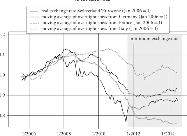
Figure 3 shows moving averages of the number of overnight stays from German, French, and Italian visitors together with monthly averages of the real exchange rate between Switzerland and the Eurozone. Both time series are indexed to 1 for January 2006. The Swiss franc depreciated against the euro from a monthly average of 1.55 CHF/EUR in January 2005 to 1.67 CHF/EUR in October 2007. Alongside this depreciation, the number of overnight stays from guests of all three neighbouring countries increased.
of the financial crisis than France and Italy. Particularly for Italy a part of the decrease in overnight stays is therefore likely to be attributed to the contraction in real GDP. By contrast, real GDP growth probably cushioned the still large fall in overnight stays from German visitors.
minimum exchange rate
1/2006 1/2008 1/2010 1/2012 1/2014 1.2
1.1
1.0
0.9
0.8
real exchange rate Switzerland/Eurozone (Jan 20061) moving average of overnight stays from Germany (Jan 20061) moving average of overnight stays from France (Jan 20061) moving average of overnight stays from Italy (Jan 20061)
Figure : Correlation between the Real Exchange Rate and Overnight Stays in the Euro Area
Several months after the SNB introduced the minimum exchange rate of 1.20 CHF/EUR, the downward trend in the moving averages of overnight stays is halted. Special care should, however, be taken by drawing a conclusion to the exact lag size as the moving average process also takes future and past values into account.
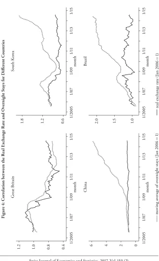
1. 2 1. 0 0. 8 0. 4 Fi g u re : C o rr el at ion b et w ee n t h e R ea l E xc h an ge R at e a n d O ve rn ig h t St ay s f o r Di ff er en t C ou n tr ie s mov in g ave ra
ge of ove
rn ig h t s tay s ( Ja n 2 0 0 6 1) re al e xc h an ge r at e ( Ja n 2 0 0 6 1) mo n th 1/ 2 0 0 5 1/ 0 7 1/ 0 9 1/ 11 1/ 13 1/ 15 Gr ea t Br it ai n 1. 8 1. 2 0. 6 mo n th 1/ 2 0 0 5 1/ 0 7 1/ 0 9 1/ 11 1/ 13 1/ 15 S out h K o re a
6 4 2 0
KRW in March 2009 is followed by a sharp decline in the number of overnight stays, while the time series otherwise shows a clear upward trend. The graph for Brazil shows a similar though less pronounced picture. The graph for China shows a six-fold increase in the number of overnight stays from Chinese visitors. However, the graph does not present a link between the two variables since the vertical axis is scaled to capture the surge in overnight stays rather than the vola-tility in the real exchange rate.
4. Empirical Approach
To estimate the elasticity of overnight stays to a change in the real exchange rate we use a log-log model, which can be derived from the theory of international tourism demand (Song, Witt, and Li, 2009). Using triple-indexed panel data we estimate the following specification, where N denotes the number of overnight stays in community i from guests of country j at month t:
ln( ) ( )ln( )
ln( )
, , , , ,
, ,
N R
Y
i j t c d j t p
j t p i t i
= + +
+ − + + −
α β ϕ β ϕ
γ 1 1 ψ2 2μ,, ,j s+εi j t, ,
(2)
R represents the average real exchange rate between country j and Switzerland (CHF per unit of foreign currency such that a decrease in R represents an appre-ciation of the Swiss franc vis-à-vis the currency of country j ), which we lag by p months. The term Y is country j’s output, i.e. its real GDP. is the coefficient for the general elasticity of overnight stays to movements in the real exchange rate.
1 are mutually exclusive binary variables, which are set to one if a community
falls within a specific category c, as defined in the next section. 1 are the
esti-mated coefficients on interaction terms between the binary variables 1 and the
real exchange rate. Similarly, 2 are mutually exclusive binary variables, which
are set to one if a country belongs to a specific continent d. 2 are the estimated
As long as hotels do not vary their level of price-discrimination across countries, the time-community fixed effects also capture price changes on the supply side, i.e. they control for an increase or decrease in the prices for overnight stays and other tourism related services. This is important as the industry is likely to react to an exchange rate change by adjusting prices. Not controlling for these supply side effects would therefore result in omitted variable bias. If hotels react to move-ments in the exchange rates by adopting prices individually by country of origin, then my results would be downward biased. However, given the importance of international booking portals, country-specific price discrimination is increas-ingly hard to enforce. µ are community-country-pair-seasonality fixed effects. They control for unobserved effects in the communities, the countries of origin as well as peculiarities in the country-community pair. Furthermore, they also account for spatial dependence by capturing neighbourhood effects. Including the community-country-pair fixed effects for each month of the year, as denoted by the subscript s, further captures the time series-specific seasonalities.
The included fixed effects are large in number. Capturing the seasonality for every community-country pair requires almost 100’000 coefficients and the time fixed effects for every community consist of another 16’000. As the data includes more than 830’000 observations, the loss in degrees of freedom causes much less of a problem than limits in the computational power. Correia (2014) developed a new algorithm for Stata which performs linear regressions while absorbing high-dimensional fixed effects. The algorithm is much faster than the hitherto available alternatives and enables us to include all of the fixed effects. Omitting the time-community fixed effects would result in a strong upward bias, while not controlling for the unobserved time-invariant characteristics of the country-community pairs would lead to a downward bias.
Entorf (1997) shows that the phenomenon of spurious regression results also applies to nonstationary panel time series models. Our panel unit root tests are not conclusive due to the weak power of these tests for the small time period of 10 years. In our case the problem is mitigated by the fact that the number of country-community pairs in the triple-indexed panel largely exceeds the number of observations in the time series dimension. However, to some extend the prob-lem might persists.
2009). However, it is not possible to take the logarithm of zero. The advantages of the log-log transformation therefore come with the disadvantage of having to deal with the zeros.
Simply dropping all values with zero observation is not an option. A possibil-ity would be to use a count model. In fact our data fulfil the two major assump-tions of count models: the observaassump-tions are non-negative and there is no natural a priori upper bound. Our data suffer from large over-dispersion, i.e. the condi-tional variance is larger than the condicondi-tional mean. This would require a (zero-inflated) negative-binominal rather than a poisson model. However, Allision and Waterman (2002), Guimarães (2008), and Greene (2007) state that the conditional maximum likelihood estimator used for negative binominal regres-sions does not qualify as a true fixed effects estimator. Furthermore, an uncondi-tional estimation of the negative binominal model by explicitly including dummy variables is not a feasible approach given the large number of coefficients which would be needed. Moreover, we consider the Poisson pseudo-maximum likeli-hood (PPML) estimator (Santos Silva and Tenreyro, 2006), which is often suggested in the international trade literature to estimate gravity models. How-ever, the PPML estimator cannot be used with high-dimensional fixed effects. We therefore follow Baldwin and Di Nino (2006) and shift the number of over-night stays by one. Baldwin and Di Nino (2006) state that this transformation is innocuous as it corresponds to censoring the distribution to one but compen-sating the uncensored value for the shift of the censoring point.
However, there is an important source for a bias, which has to do with the weighting of the time series. While the implications for the estimated coefficients are large, the cause is rather subtle. The issue therefore deserves some explanation.
To make the point and without loss of generality we focus on the community of Davos. The lines in the top row of Figure 5 show the time series of the British and Japanese overnight stays in Davos. Unlike for Zermatt, the Japanese visitors are of minor importance for Davos and only account for a few hundred over-night stays per year. In contrast, significantly more British visit Davos. In fact, British residents are the community’s second largest group of foreign visitors. Let us now assume an alternative World as shown in the two graphs at the bottom. On the one hand, the Japanese would visit Davos almost as often as Zermatt. We therefore multiply the number of overnight stays from Japanese tourists by 10. On the other hand, we divide the number of overnight stays from British visitors by the same number. We do not change the number of overnight stays from the other 57 countries.
10 5 0 Fi g u re : L in ea r T ra n sf or m at
ion of t
h e Ob se rv at ion s i
n a S
p ec ifi c Ti me S er ie s ( q ) mo n th 1/ 2 0 0 5 1/ 0 7 1/ 0 9 1/ 11 1/ 13 1/ 15 GBR i n D avo s ( re al W o rld)
10 5 0
mo n th 1/ 2 0 0 5 1/ 0 7 1/ 0 9 1/ 11 1/ 13 1/ 15 JP N i n D avo s ( re al W o rld)
10 5 0
mo n th 1/ 2 0 0 5 1/ 0 7 1/ 0 9 1/ 11 1/ 13 1/ 15 GBR i n D avo s ( al t. W o rld)
10 5 0
estimated elasticities are exactly the same. Any country specific transformation in the number of overnight stays does not change the results. This is a conse-quence of the fixed effects model. By using the deviation from the mean it only focuses on the within variation, i.e. the variation over time.
Through the inclusion of the fixed effects we throw away all the variation across the different countries of origin. As the average is taken out, the absolute number of individuals, which make up the time series, does not have any impact on the estimated coefficients. For this reason the estimates are not sensitive to any linear transfor-mation of the observations in a specific time series. The fixed effects estimator without weights reflects a world in which an appreciation of the Swiss franc to the US dollar has ceteris paribus the same impact on the Swiss tourism industry as an appreciation of the Swiss franc to the Icelandic krona. By the same token a Maltese’s reaction to an appreciation of the euro has the same impact on the estimated coefficient as the simultaneous decisions of more than 1000 Germans.
Let us take a second look at Figure 5. When comparing the overnight stays from the two countries, we recognise a much clearer seasonal pattern for the British than for the Japanese. However, the noise in the time series of the Japanese is not the result of insane minds and continuous changes in the Japanese preferences for the ideal month for holidays in Davos. Rather it reflects the relatively low number of Japanese who actively make a decision of whether to book a hotel room in Davos or not. The information contained in the different time series is very different.
For the reasons stated above, the estimated coefficients of an unweighted fixed effects estimator depend significantly on the degree of aggregation in the data, as for example whether to aggregate the number of overnight stays of visitors from eurozone countries or not. The problem described in this section is not limited to the dimension of the countries of origin, but also exists for the different com-munities in Switzerland. The time series of Zurich and Zermatt contain more information and are more important for the Swiss tourism industry than the ones of Frutigen and Bregaglia. This paper addresses the described issue by using a weighted least squares (WLS) fixed effects estimator. By doing so we give analyti-cal weights to the different time series, which we weight by the average number of overnight stays from country j in community i:
w N
N
i j
t i j t
t i j i j t
,
, ,
, ,
= =
= = =
∑
∑ ∑ ∑
1120
1 120
1 141
1
59 (3)
that the weighting scheme is not affected by the transformation of the depen-dent variable, as the weights are taken from the original data, not those shifted by one unit.
As mentioned before, the average number of overnight stays of a specific time series is mostly determined by characteristics of the country-community pair, i.e. the between variation is much higher than the within variation. While move-ments in the Swiss franc have an impact on the number of overnight stays for the specific community-country pairs, the average nights spent in Lausanne by French guests (7’087 per month) will always be much higher than the ones spent by Finnish visitors in Weggis (7.2 per month). Nevertheless, taking the weights according to the average number of overnight stays may cause a small endoge-neity problem, as the real exchange rate might influences the average number of overnight stays for a specific country-community pair. However, the problem becomes insignificant if the real exchange rate is stationary. For two further rea-sons we prefer the average number of overnight stays to the number of a specific month: First, the country-community specific seasonalities render the number of nights of a single month less representative. Second, by choosing a single month or the average over a year we do not consider the development in the number of overnight stays for reasons other than the exchange rate.
Our method has one big disadvantage and one big advantage. The big disad-vantage is that we cannot interpret the coefficients as the impact of a specific time lag – and of only this time lag – on the number of overnight stays. The reason is again the high autocorrelation in the real exchange rate, which would cause the 1st and 2nd time lag to be significant even if all visitors had already planned their
journey to Switzerland at least 3 months in advance. The big advantage is that we omit the problem of multicollinearity. The estimated coefficients therefore provide an accurate measure for the overall impact of real exchange rate move-ments on the number of overnight stays. Nevertheless, we believe that an exten-sion to a dynamic model to account for persistence of tourism demand would be an interesting approach for future research.
5. Results
5.1 Overall Results
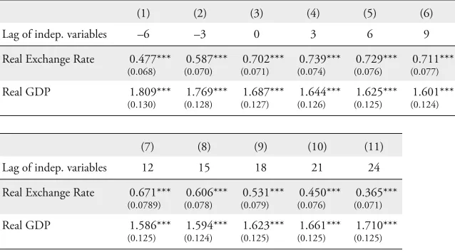
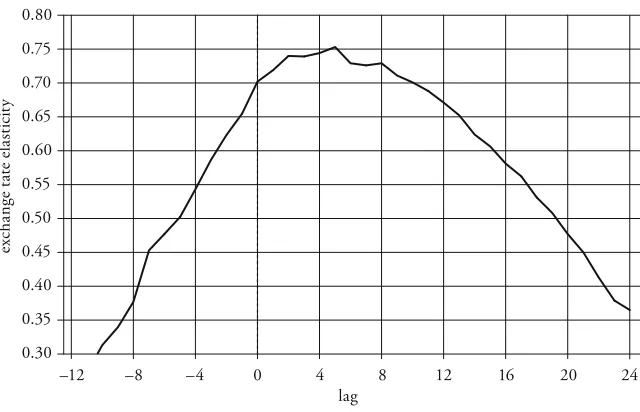
Table 1 presents the estimated coefficients for 11 regressions with 11 different time lags. Figure 6 visualises these estimates together with the estimated coeffi-cients for every other lag in the range of 12 forward and 24 backward lags. The regressions with the highest estimates for the exchange rate elasticity include lags of 3 to 5 months. The values of these coefficients are about 0.74. As we use a log-log specification we can interpret the coefficients as elasticities. A real apprecia-tion of the Swiss franc by 1% therefore leads to a decrease of 0.74% in the number of overnight stays in the 141 communities included in our sample.
On the one hand, this estimate is higher than the overall exchange rate elastici-ties of 0.53 found by Ferro Luzzi and Flückiger (2003) and of 0.57 found by Abrahamsen and Simmons-Süer (2011) when using a generalised least square model. On the other hand, our estimate is below those found by Abrahamsen and Simmons-Süer (2011) when using an error-correction model and largely below the values found by Falk (2014). In addition, our estimates are below the aver-age price elasticity for international tourism demand of 1.28 (Peng et al., 2015).
Figure 6 contains some other interesting information. As a matter of fact, current exchange rate movements do not change past numbers of overnight stays. The forward estimates on the left-hand side of the vertical line do therefore not con-tain any information about visitors’ reaction to exchange rate movements. The high estimates for the first few forward coefficients are solely the result of the high autocorrelation in the exchange rates. However, the slope of the parable is much lower on the right-hand side than on the left-hand side, i.e. for the back-ward lags than for the forback-ward lags. While most visitors react to the exchange rate 3 to 5 months in advance of their actual visit, the lower slope on the right indi-cates that further backward lags still matter. Explanations are manifold: visitors often have an incentive for early bookings of flights, hotels, or travel packages due to the pricing system of airlines and travel agencies, or in order to ensure their spots in their favourite hotel or travel group. Through early bookings and pay-ment in their home currency, visitors might also transfer a part of the exchange rate risk to other parties.
Table 1: Overall Findings
Dependent variable: log of overnight stays
Independent variable: log of the real exchange rate CHF/local currency; index Jan2005 1 Control variable: real GDP in local currency; index: Jan2005 1
(1) (2) (3) (4) (5) (6)
Lag of indep. variables –6 –3 0 3 6 9
Real Exchange Rate 0.477***
(0.068)
0.587***
(0.070)
0.702***
(0.071)
0.739***
(0.074)
0.729***
(0.076)
0.711***
(0.077)
Real GDP 1.809***
(0.130)
1.769***
(0.128)
1.687***
(0.127)
1.644***
(0.126)
1.625***
(0.125)
1.601***
(0.124)
(7) (8) (9) (10) (11)
Lag of indep. variables 12 15 18 21 24
Real Exchange Rate 0.671***
(0.0789)
0.606***
(0.078)
0.531***
(0.079)
0.450***
(0.076)
0.365***
(0.071)
Real GDP 1.586***
(0.125)
1.594***
(0.124)
1.623***
(0.125)
1.661***
(0.125)
1.710***
(0.125)
We find elasticities of overnight stays with respect to real GDP between 1.6 and 1.8. An increase of real GDP by 1% therefore leads to an increase in the number of overnight stays of about 1.6 to 1.8%. Peng et al. (2015) report a median income elasticity of 2.53. While we find lower values, our income elasticities are still significantly above one. Therefore, we agree with the conclusion made by Peng et al. (2015) that international tourism is clearly a luxury product.
5.2 Country Results
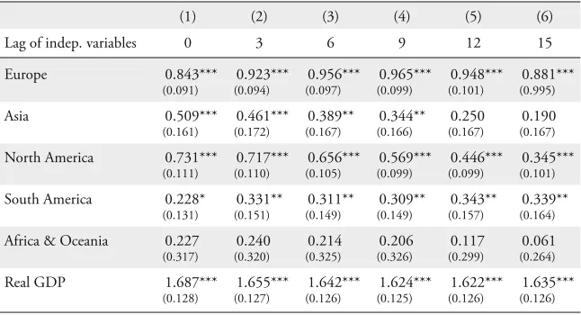
Table 2 presents the estimated coefficients from interacting the real exchange rate with a categorical variable, which groups the countries by their continent.
For the remainder of the paper we drop , the coefficient for the overall elas-ticity of overnight stays to movements in the real exchange rate. Therefore we can directly read the coefficients on the interaction terms as the exchange rate elasticities for the different continents. Table 2 presents the estimated coefficients for time lags of 0, 3, 6, 9, 12 and 15 months. The estimated elasticity for Euro-pean visitors peaks at a value of slightly below 1. A real appreciation of the Swiss franc by 10% therefore leads to a drop in the number of overnight stays from European countries by about 9.7%. This elasticity is higher than the ones of any
0.80
0.75
0.70
0.65
0.60
0.55
0.50
0.45
0.40
0.35
0.30
–12 –8 –4 0 4 8 12 16 20 24
lag
ex
ch
an
ge
t
at
e ela
st
ici
ty
other country group. The highest coefficient for visitors from North America is about 0.73, while the elasticities for the other country groups are much lower.
In general we observe higher elasticities for countries which are geographically closely located to Switzerland. This indicates that the ratio between the distance from the country of origin to Europe and Europe to Switzerland is important. One reason might be found in the transportation and opportunity costs of trav-elling. The implicit and explicit transportation costs between Swiss and other European destinations are often low compared to the costs and the needed time to travel from other continents to Europe. For visitors from outside of Europe, Swiss and European tourism therefore might be complementary goods. Once these tourists are already in Europe, the relative costs and time needed to visit a Swiss destination is low. For these visitors the euro might even play a bigger role than the Swiss franc, though the latter still matters. The situation is different for Europeans. Once the high fixed cost for the transport to Europe falls away, European and Swiss destinations are likely to become substitution goods. This
Table 2: Country Group Findings
Dependent variable: log of overnight stays
Independent variable: log of the real exchange rate CHF/local currency; index Jan2005 1 Control variable: real GDP in local currency; index: Jan2005 1
(1) (2) (3) (4) (5) (6)
Lag of indep. variables 0 3 6 9 12 15
Europe 0.843*** (0.091) 0.923*** (0.094) 0.956*** (0.097) 0.965*** (0.099) 0.948*** (0.101) 0.881*** (0.995) Asia 0.509*** (0.161) 0.461*** (0.172) 0.389** (0.167) 0.344** (0.166) 0.250 (0.167) 0.190 (0.167)
North America 0.731***
(0.111) 0.717*** (0.110) 0.656*** (0.105) 0.569*** (0.099) 0.446*** (0.099) 0.345*** (0.101)
South America 0.228*
(0.131) 0.331** (0.151) 0.311** (0.149) 0.309** (0.149) 0.343** (0.157) 0.339** (0.164)
Africa & Oceania 0.227
(0.317) 0.240 (0.320) 0.214 (0.325) 0.206 (0.326) 0.117 (0.299) 0.061 (0.264)
Real GDP 1.687***
(0.128) 1.655*** (0.127) 1.642*** (0.126) 1.624*** (0.125) 1.622*** (0.126) 1.635*** (0.126)
is particularly true for destinations in neighbouring countries, which often offer similar services. In addition, Crouch (1994) states that a destination might become more attractive and more luxurious with distance. Price elasticities would therefore be lower for long-haul tourism as the longer the distance the more lux-urious the tourism.
While there are many explanations for the different estimates across countries and country-groups, the coefficients of the different time lags within countries and country-groups are harder to explain. Intuitively, we would expect visitors from Europe to react with a shorter time lag to exchange rate movements, as they probably plan their trips less in advance. This is, however, not the case. Euro-pean visitors seem to react with a larger time lag to movements in the Swiss franc than European guests. An explanation might be that a large part of non-European visitors, when planning their journey, actually reacts to movements in the euro, rather than in the Swiss franc. Once they are in Europe, however, the Swiss franc might become a decision criteria on whether to visit a Swiss destina-tion or not. An appreciadestina-tion of the Swiss franc may also incline visitors to reduce the number of overnight stays per arrival.
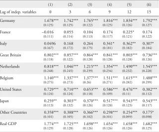
Table 3 presents country specific exchange rate elasticities for the 8 countries with the most overnight stays during the observation period. The findings for European countries confirm the impression obtained from Figure 3: differences across Europe’s main visitor countries are large. In particular the German, Dutch, and Belgian markets are highly price sensitive. A real appreciation of the Swiss franc by 10% decreases the number of overnight stays from Dutch and Belgian visitors by more than 15% and from German visitors by more than 18%. By con-trast, Italian and particularly French visitors react much less to exchange rate changes. In fact, even the largest coefficient for the French market is only sig-nificant at the 10% significance level. Our findings stay in contrast to the results reported by Abrahamsen and Simmons-Süer (2011), which find very high real exchange rate elasticities of 2.32 for French and 1.96 for Italian visitors, albeit for a different time period.
5.3 Community Group Results
The preceding sections provide estimates for the elasticity of overnight stays to movements in the real exchange rate for Switzerland as a whole. The results of the last section further show the importance of the source market. While some deter-minants of the visitors’ price sensitivity such as implicit and explicit transport costs are mainly connected to the visitors’ country of origin, others are mainly connected to the specific destination within Switzerland itself. Examples are the
Table 3: Country Findings
Dependent variable: log of overnight stays
Independent variable: log of the real exchange rate CHF/local currency; index Jan2005 1 Control variable: real GDP in local currency; index: Jan2005 1
(1) (2) (3) (4) (5) (6)
Lag of indep. variables 0 3 6 9 12 15
Germany 1.678*** (0.125) 1.742*** (0.125) 1.765*** (0.122) 1.816*** (0.125) 1.834*** (0.126) 1.792*** (0.127) France –0.016 (0.111) 0.055 (0.114) 0.104 (0.113) 0.174 (0.117) 0.225* (0.121) 0.174 (0.122) Italy 0.0496 (0.167) 0.168 (0.172) 0.264 (0.175) 0.341* (0.181) 0.362** (0.182) 0.307* (0.184)
Great Britain 0.802***
(0.118) 0.857*** (0.122) 0.864*** (0.128) 0.841*** (0.128) 0.803*** (0.128) 0.736*** (0.126) Netherlands 0.818*** (0.248) 1.046*** (0.245) 1.215*** (0.239) 1.354*** (0.234) 1.490*** (0.232) 1.545*** (0.228) Belgium 1.140*** (0.275) 1.337*** (0.273) 1.377*** (0.26) 1.511*** (0.271) 1.615*** (0.282) 1.488*** (0.299)
United States 0.729***
(0.124) 0.710*** (0.124) 0.653*** (0.118) 0.586*** (0.109) 0.476*** (0.11) 0.382*** (0.112) Japan 0.259** (0.113) 0.303** (0.132) 0.370*** (0.126) 0.517*** (0.128) 0.543*** (0.123) 0.543*** (0.117)
Other Countries 0.358***
(0.101) 0.388*** (0.105) 0.366*** (0.102) 0.298*** (0.101) 0.254*** (0.099) 0.175* (0.098)
Real GDP 1.774***
(0.129) 1.725*** (0.128) 1.698*** (0.126) 1.654*** (0.126) 1.658*** (0.126) 1.682*** (0.125)
4 Official spatial division by the FSO; Community-types 9 of the year 2000.
price category of hotels or the visitors purpose to stay in Switzerland. Country-wide results are likely to conceal these community-specific disparities. In what follows, we therefore investigate the impact of exchange rate movements depen-dent on different community-specific characteristics.
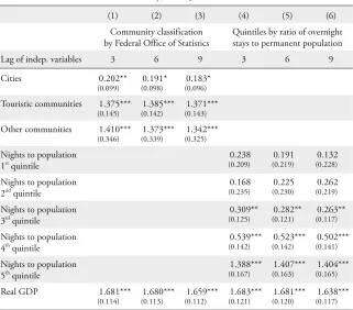
One important factor, which is likely to determine the price sensitivity of visi-tors, is their purpose for staying in Switzerland. Unfortunately, there exists no data on the guests’ purpose of visit. Therefore, we cannot estimate different elas-ticities by the visitors’ purpose of staying in a specific community directly. How-ever, observable community characteristics provide good indicators for the guests’ main purpose of visit. We use an official classification into 9 different commu-nity-types4 by the FSO to construct a community-type categorical variable. 44 out of the 141 communities in our sample are classified as cities, 59 as touristic communities and 38 belong to one of the other categories. The first 3 columns in Table 4 show the estimated coefficients from interacting the community-type categorical variable with the logarithm of the real exchange rate. We report the 3rd, 6th, and 9th time lag, as the impact of a change in the exchange rate peaks with a lag of one to three quarters. The differences in the elasticities between cities and the two other types of communities are large. An appreciation of the Swiss franc by 10% leads, on the one hand, to a decrease in the number of overnight stays form foreign visitors in touristic and other communities of about 14%. On the other hand, the same appreciation of the Swiss franc decreases the number of overnight stays in cities by only 2%. The estimated coefficients for cities are further only significant at the 10% level in two out of three cases.
The above analysis shows the relatively large effect of exchange rate movements on the Swiss tourism industry. As previously noted, there is a strong degree of season-ality with two peak seasons: one in summer from June to August and one in winter from December to March. The seasonality patterns are much less pronounced for cities than for touristic communities. The patterns of the latter are further very community specific. Some accommodate almost all of their guests in either winter or summer, others have a high and a middle season. How do exchange
Table 4: Tourism Intensity of Communities
Dependent variable: log of overnight stays
Independent variable: log of the real exchange rate CHF/local currency; index Jan2005 1 Control variable: real GDP in local currency; index: Jan2005 1
(1) (2) (3) (4) (5) (6)
Community classification by Federal Office of Statistics
Quintiles by ratio of overnight stays to permanent population
Lag of indep. variables 3 6 9 3 6 9
Cities 0.202** (0.099) 0.191* (0.098) 0.183* (0.096)
Touristic communities 1.375***
(0.145)
1.385***
(0.142)
1.371***
(0.143)
Other communities 1.410***
(0.346)
1.373***
(0.339)
1.342***
(0.325)
Nights to population 1st quintile 0.238 (0.209) 0.191 (0.219) 0.132 (0.228)
Nights to population 2nd quintile 0.168 (0.235) 0.225 (0.230) 0.262 (0.219)
Nights to population 3rd quintile 0.309** (0.125) 0.282** (0.121) 0.263** (0.117)
Nights to population 4th quintile 0.539*** (0.142) 0.523*** (0.142) 0.502*** (0.141)
Nights to population 5th quintile 1.388*** (0.167) 1.407*** (0.163) 1.404*** (0.165)
Real GDP 1.681***
(0.114) 1.680*** (0.113) 1.659*** (0.112) 1.683*** (0.121) 1.681*** (0.120) 1.638*** (0.117)
rate movements affect these different types of communities? Is the effect of the exchange rate different for summer and winter tourism? The second question is difficult to answer because of the relatively long and not exactly defined transmis-sion period of a change in the exchange rate on the number of overnight stays. To answer the first question, we exploit the seasonal pattern in the time series of the communities. For each community we calculate the number of overnight stays during the winter, respectively summer months, as a share of average annual over-night stays. Just as with the ratio for the tourism-intensity, we rank the communi-ties by the obtained ratios. Subsequently we create a dummy variable for the first quartile, or the first 35 communities, of each ranking. The winter destinations of the first quartile count 43% or more of their overnight stays between December and March. The most specialised community is Bagnes in the canton of Valais, which counts 73% of overnight stays by foreigners during the winter season. It is followed by Tujetsch (71%) and Nendaz (68%). 35 summer destinations count at least 41% of their international hotel nights in June, July, or August. With 60% Innertkirchen is at the top of the list, followed by Ringgenberg (59%) and Val Müstair (57%). As guests are much more equally distributed across months in cities compared to touristic destinations, both, summer and winter destinations, do not include any cities. This is desired as cities have much lower elasticities for reasons discussed above. Excluding cities enables us to look at the different effects of exchange rate movements within non-city destinations. In fact, the need to exclude cities is the main reason why we chose the top quartile, rather than ter-tile. Defining the summer and winter destinations as the top quartile allows us to exclude all cities, while including almost all tourism destinations.
Does a change in the exchange rate have a different effect on the number of over-night stays in more luxurious and prestigious destinations? Intuitively we would expect more wealthy guests to reveal a lower exchange rate elasticity. However, the only study we are aware of claims the opposite. Corgel, Lane, and Walls (2013) estimate the effect of exchange rate movements on the demand for hotel rooms of different price classes in the US. The authors find significantly higher elasticities for luxury and upscale hotels. Our data does not contain a breakdown by the price category or the number of stars.
However, community level data allows us to compare destinations of different price levels. The preceding analysis showed large differences in the elasticities between cities and non-cities and, within the latter, between summer and winter destinations. The price level of communities is related to these groups. In fact, cities count 38 and winter destinations 28 five Star hotels, while there are only 6 five star hotels in summer destinations. Therefore, we do not want to com-pare destinations across the different categories. For this reason, this paper only compares more luxurious destinations against other destinations within, but not across, the summer and winter community groups. For this part of the analysis,
Table 5: Seasonal Specialisation of Communities
Dependent variable: log of overnight stays
Independent variable: log of real exchange rate CHF/local currency; index Jan2005 1 Control variable: log of real GDP in local currency; Index: Jan2005 1
(1) (2) (3) (4) (5)
Lag of the independent variables 0 3 6 9 12
Specialised in winter tourism (December to March)
0.862***
(0.121)
0.974***
(0.125)
0.998***
(0.134)
1.007***
(0.145)
0.966***
(0.153)
Specialised in summer tourism (June to August)
2.031***
(0.445)
2.092***
(0.449)
2.128***
(0.433)
2.113***
(0.423)
2.125***
(0.407)
Other communities 0.447***
(0.085)
0.459***
(0.087)
0.436***
(0.087)
0.415***
(0.086)
0.375***
(0.086)
Real GDP 1.700***
(0.123)
1.661***
(0.122)
1.643***
(0.121)
1.620***
(0.120)
1.605***
(0.120)
we do not consider any communities other than the ones in these two groups. To obtain a measure for the price category, we use the hotel directory on the website of myswitzerland.com to create a list of 4 and 5 star hotels in each community. Subsequently, we use this list to create an index for the average price level of the hotels in a community. We calculate the index as the ratio of 4 and 5 star to the number of total hotels, while multiplying 5 star hotels by 5. The idea is to base the index principally on 5 star, while complementary considering 4 star hotels. While the hotel directory of myswitzerland.com offers a comprehensive list of middle and upscale hotels, many low price hotels are missing. Fortunately, the FSO provides data on the number of hotels in each community. We use this data as denominator. In the spirit of the preceding analysis, we rank the communities by the described index and create a dummy variable for the communities of the first quintile of the ranking. The number of communities in the high-price seg-ment is therefore relatively small. However, on average these communities count more overnight stays than non-luxury destinations.
Table 6 presents the estimated coefficients from interacting the exchange rate with the dummy variable for luxurious communities and, to compare the com-munities within categories, with the categorical variable for summer and winter destinations. Again, since all variables are in logarithms, we can interpret the coefficients as elasticities. Compared to the base group, the estimated coeffi-cients are slightly lower for high-price destinations. The effect of exchange rate movements therefore tends to be lower for more luxury and upscale destinations with a relatively high number of 4 and particularly 5 star hotels. This is true for summer and winter destinations. However, the difference in the estimates within the summer and winter groups is small and the 5 percent confidence intervals are overlapping. Whether a community is primarily a winter or summer destination is therefore more important than the average price class of the hotels. Degree of competition might be less pronounced in Alpine destinations than in summer destinations. However, it is important to mention that our analysis is based on community characteristics, and not on the data of individual hotels. This restric-tion becomes important for the estimated coefficients in Table 6, as most luxury destinations also include less expensive hotels and vice versa.
6. Conclusion and Discussion
of 0.74. Put differently, an appreciation of the Swiss franc by 10% decreases the number of international overnight stays in Swiss hotels by 7.4%. Disaggregated data for 141 communities and 59 countries of origin allowed us to estimate coun-try and community-specific exchange rate elasticities. In both dimensions, we found large differences in the estimated elasticities across groups.
With respect to the country of origin, we found very high exchange rate elas-ticities for German, Dutch, and Belgian visitors. A 10% appreciation of the Swiss franc against the euro reduces the number of overnight stays from Dutch and Belgian visitors by more than 15% and from German visitors by more than 18%. By contrast, Italian and particularly French visitors exhibit a very low price sensi-tivity. Guests from North America and Asia exhibit exchange rate elasticities of 0.73 and 0.51 respectively. For guests from South America, Africa, and Oceania the estimated values are much lower or insignificant.
Table 6: Customer Segment of Communities
Dependent variable: log of overnight stays
Independent variable: log of real exchange rate CHF/local currency; index Jan2005 1 Control variable: log of real GDP in local currency; index: Jan2005 1
(1) (2) (3) (4) (5)
Lag of indep. variables 0 3 6 9 12
no. com-munities
Winter destinations
high-price segment 9 0.806***
(0.154)
0.915***
(0.163)
0.971***
(0.179)
0.981***
(0.201)
0.931***
(0.215)
other 26 0.960***
(0.169)
1.080***
(0.173)
1.059***
(0.182)
1.067***
(0.193)
1.038***
(0.191)
Summer destinations
high-price segment 5 1.880**
(0.827)
1.991**
(0.841)
2.118***
(0.824)
2.066***
(0.787)
1.993**
(0.804)
other 30 2.054***
(0.472)
2.113***
(0.477)
2.142***
(0.459)
2.129***
(0.449)
2.147***
(0.433)
Real GDP 2.054***
(0.472)
2.113***
(0.477)
2.142***
(0.459)
2.129***
(0.449)
2.147***
(0.433)
With respect to the communities, we found very low elasticities of 0.2 for cities but very high values of 1.4 for rural communities. By the same token, exchange rate movements have a higher effect in communities with a high number of overnight stays relative to the permanent population. While there exists no data on the guests’ purpose of visit, these findings indicate a higher price sensitivity of holiday tourists compared to business travellers. Within rural communities, exchange rate movements have a much larger effect on summer than on winter destinations. The elasticity for communities, which accommodate a large part of their guests in summer, is slightly above 2 and therefore about twice as high as the estimated coefficient for winter destinations. For both, summer and winter destinations, exchange rate movements tend to have a lower impact on overnight stays in more upscale and luxury destinations with a high share of 4, and partic-ularly 5 star hotels. However, the difference to the base group of less expensive destinations is not significant.
What do these findings tell us about the effect of the central bank’s decision to remove the exchange rate floor? How do the findings contribute to the ongo-ing policy debate?
The impact of the strong Swiss franc on the tourism industry strongly depends on community characteristics:
The Swiss franc’s appreciation has a small impact on the number of overnight stays in cities. About one year after the SNB removed the exchange rate floor, one euro costs about one franc and eight cents. Compared to an exchange rate of 1.20 CHF/EUR, the Swiss franc therefore appreciated by about 10%. Everything else constant, this should reduce the number of international overnight stays in cities by about 2%. For the 44 communities, which the FSO classifies as cities, this is equivalent to a loss of about 12’000 international overnight stays per month.
While the impact of a change in the exchange rate is small for cities, it is large for all other communities. For these communities we found elasticities of about 1.4. A real appreciation of the Swiss franc by 10%, therefore decreases the number of international overnight stays in these communities by about 14%. For the 97 rural communities included in this paper, this is equivalent to a loss of about 75’000 international overnight stays per month. However, price sensitivities are highly heterogeneous across source markets.
of the exchange rate shock might also depends on the possibility for regional-specific solutions within the sector’s collective labour agreement. On the side of hotels, price discounts might be targeted to source markets with a high price sen-sitivity. Moreover, hotel chains can mitigate the effect of exchange rate changes through the diversification of hotel locations across rural and urban communities.
While the appreciation has a large negative impact on rural communities, sev-eral factors should mitigate the impact of the exchange rate appreciation:
First, this paper aimed to estimate the ceteris paribus effect of a change in the real exchange rate. Even if the strong appreciation of the Swiss franc has ceteris paribus a negative effect, this does not mean that the number of international overnight stays will actually decrease in the long run. Over time, expected real growth in the visitors’ countries of origin is likely to compensate for the nega-tive effect of the Swiss franc’s appreciation. However, real growth in the visitors’ countries of origin is taking place gradually and cannot counter a shock suffi-ciently. Nevertheless, during the last 10 years real growth caused the number of overnight stays for many of the visitors countries of origin to follow a clear upward trend. The most striking example is the development in the number of overnight stays from Chinese visitors.
Second, since January 2015 many currencies such as the British pound and the US dollar have appreciated against the euro. This would also have been the case if the SNB had decided to keep defending the exchange rate floor. Never-theless, currencies other than the euro cause the appreciation of the real effective exchange rate to be below the mentioned 10%, which the Swiss franc appreci-ated against the euro.
Appendix
0 10 20 30 40 50 Overnight stays
Range from 0 to 50
0 10 20 30 40 50 Overnight stays103
Total range, excluding 0
4.0
3.0
2.0
1.0
0 Frequency105
Figure : Overnight Stays: Distribution of the Observations
0 5 10 15 20
lag Bartlett’s formula for MA(q) 95% confidence bands
0 5 10 15 20
lag 95% Confidence bands Autocorrelations of R
between Switzerland and Germany
Partial autocorrelations of R between Switzerland and Germany 1.0
0.5
0.0
–0.5
–1.0
1.0
0.5
0.0
–0.5
SE1 n
[ ]
0
25
50
16.
0
8.
0
–
15
.9
6
.0
–
7.9
4.
0
–
5
.9
2
.0
–
3
.9
1.
0
–
1.
9
0
.5
–0
.9
0
.5
km
N
u
mb
er
of Hot
el
s
/1
0
0
0
I
n
h
abi
ta
n
ts
Fi
g
u
re
: N
u
mb
er
of Hot
el
s p
er
I
n
h
abi
ta
n
Table 7: Average International Overnight Stays per Month in the 141 Communities
Municipality average nights / month
Municipality average nights / month
Municipality average nights / month
Zurich 156’542 Ingenbohl 4’580 Arbon 1’462
Geneva 115’162 Kandersteg 4’505 Kreuzlingen 1’454
Zermatt 62’562 Vaz/Obervaz 4’479 Sarnen 1’449
Lucerne 58’871 Baden 4’020 Bellinzona 1’412
Basel 56’725 Celerina/Schlarigna 3’955 La
Chaux-de-Fonds 1’362 St. Moritz 43’229 Saas-Grund 3’943 Mendrisio 1’330
Davos 38’397 Fribourg 3’908 Aarau 1’320
Interlaken 37’193 Biel/Bienne 3’804 Stein am Rhein 1’208
Lausanne 37’039 Schaffhausen 3’568 Flums 1’189
Lauterbrunnen 29’163 Hasliberg 3’409 Flühli 1’189
Berne 28’269 Andermatt 3’228 Bulle 1’185
Grindelwald 28’103 Morschach 3’170 Frauenfeld 1’179
Lugano 25’370 Champèry 3’116 Ringgenberg
(BE)
1’172
Meyrin 20’655 Ormont-Dessus 3’061 Fiesch 1’159
Montreux 18’467 Sachseln 3’031 Uzwil 1’144
Engelberg 18’037 Thun 2’996 Aeschi bei Spiez 1’124
Saas-Fee 16’641 Muralto 2’957 Murten 1’081
Ascona 13’588 Quarten 2’956 Schwende 1’023
Pontresina 13’455 Morges 2’782 Airolo 985
Ollon 13’278 Scuol 2’754 Nendaz 972
Klosters-Serneus 10’440 Nyon 2’744 Glarus Süd 960
Saanen 10’082 Matten bei Interlaken 2’509 Poschiavo 905
Paradiso 9’891 Küssnacht (SZ) 2’461 Appenzell 888
Bagnes 8’796 Orsières 2’403 Château-d'Oex 857
Anniviers 8’733 Disentis/Mustér 2’383 Gersau 843
Laax 8’206 Solothurn 2’382 Langenthal 798
Leysin 8’105 Rapperswil-Jona 2’289 Sierre 758
Municipality average nights / month
Municipality average nights / month
Municipality average nights / month
Chur 7’017 Vitznau 2’153 Wil (SG) 724
Samnaun 7’007 Spiez 2’149 Reichenbach
i.K.
714
Brig-Glis 6’959 Sion 2’136 Altstätten 669
Unterseen 6’874 Freienbach 2’121 Schwyz 655
Winterthur 6’749 Kerns 2’086 Glarus Nord 636
Zug 6’649 Sigriswil 2’051 Innertkirchen 629
St. Gallen 6’589 Olten 1’988 Heiden 597
Locarno 6’446 Dübendorf 1’839 Zweisimmen 578
Bad Ragaz 6’396 Samedan 1’777 Delèmont 543
Adelboden 5’684 Bad Zurzach 1’734 Breil/Brigels 525
Beatenberg 5’679 Bregaglia 1’701 Sursee 515
Weggis 5’614 Lenk 1’661 Val Müstair 424
Leukerbad 5’586 Brienz (BE) 1’650 Unterägeri 392
Vevey 5’428 Wildhaus-Alt St. Johann 1’630 Herisau 384
Wilderswil 5’383 Zernez 1’570 Frutigen 311
Montana 4’991 Gambarogno 1’555 Arth 304
Neuchâtel 4’862 Tujetsch 1’541 Plaffeien 294
Meiringen 4’690 Beckenried 1’490 Twann-Tüscherz 238
Martigny 4’610 Evolène 1’472 Amden 221
Table 8: Average Overnight Stays per Month from the 59 Countries
Country average nights / month
Country average nights / month
Country average nights / month
DEU 302’786 ARE 11’069 IDN 2’977
GBR 135’660 DNK 7’645 MEX 2’691
USA 108’137 LUX 7’599 EGY 2’629
FRA 82’735 GRC 7’440 BGR 2’305
ITA 64’221 SGP 7’362 SVK 1’737
NLD 49’063 POL 7’319 HRV 1’482
BEL 43’460 NOR 6’902 SVN 1’403
JPN 38’938 PRT 5’982 BHR 1’391
RUS 33’551 TUR 5’819 NZL 1’260
CHN 30’198 FIN 5’801 PHL 1’155
ESP 27’828 IRL 5’331 EST 1’117
IND 25’736 CZE 5’328 OMN 1’116
AUT 21’327 HKG 5’252 BLR 881
AUS 15’273 ROU 4’866 LTU 838
CAN 14’721 ZAF 4’691 ISL 819
SAU 13’717 UKR 4’415 LVA 737
SWE 13’519 HUN 4’171 SRB 710
KOR 11’814 KWT 3’800 CYP 674
BRA 11’627 QAT 3’484 MLT 503
ISR 11’173 MYS 3’439
Table 9: Autocorrelation Function (AC) and Partial Autocorrelation Function (PAC) between Switzerland and Germany
Lag AC PAC
1 0.9808 0.9889
2 0.9612 –0.0142
3 0.9450 0.1018
4 0.9273 –0.0793
5 0.9133 0.1180
6 0.8991 –0.0915
7 0.8830 –0.0007
8 0.8597 –0.2852
9 0.8341 –0.0727
10 0.8120 0.0259
11 0.7901 0.0078
12 0.7661 –0.1315
13 0.7393 –0.1217
14 0.7137 0.0370
15 0.6862 –0.0279
16 0.6584 0.0199
17 0.6319 –0.0386
18 0.6040 –0.0218
19 0.5771 0.1011
Table 10: Overall Findings with More than One Lag
Dependent variable: log of overnight stays
Independent variable: log of the real exchange rate CHF/lcu Control variable: real GDP in local currency; index: Jan2005 1
(2) (3) (4) (5) (6)
R: L1 0.321***
(0.08)
0.412***
(0.063)
0.444***
(0.05)
R: L2 0.178*
(0.091)
R: L3 –0.083
(0.093)
–0.066
(0.065)
0.490***
(0.055)
R: L4 –0.190*
(0.105)
0.442***
(0.057)
R: L5 0.600***
(0.117)
0.281***
(0.062)
R: L6 –0.359***
(0.112)
0.116***
(0.044)
–0.044
(0.053)
R: L7 –0.082
(0.1)
–0.099*
(0.06)
R: L8 0.342***
(0.108)
0.366***
(0.077)
R: L9 –0.219**
(0.1)
0.010
(0.062)
0.397***
(0.08)
R: L10 0.125
(0.119)
R: L11 –0.078
(0.113)
0.375***
(0.085)
R: L12 0.373***
(0.106)
0.365***
(0.072)
GDP: L6 1.532***
(0.13)
1.541***
(0.129)
1.533***
(0.13)
1.573***
(0.127)
1.588***
(0.126)