On the reliability and availability of replicated and rejuvenating systems under stealth attacks and intrusions

DOI 10.1007/s13173-012-0062-x L A D C 2 0 1 1

On the reliability and availability of replicated and rejuvenating

systems under stealth attacks and intrusions

Luís Teixeira d’Aguiar Norton Brandão· Alysson Neves Bessani

Received: 19 September 2011 / Accepted: 28 January 2012 / Published online: 1 March 2012 © The Brazilian Computer Society 2012

Abstract This paper considers the estimation of reliability and availability of intrusion-tolerant systems subject to non-detectable intrusions caused by stealth attacks. We observe that typical intrusion tolerance techniques may in certain cir-cumstances worsen the dependability properties they were meant to improve. We model intrusions as a probabilistic effect of adversarial efforts and analyze different strategies of attack and rejuvenation. We compare several configura-tions of intrusion-tolerant replication and proactive rejuve-nation, and varying mission times and expected times to node-intrusion. In doing so, we identify thresholds that dis-tinguish between improvement and degradation of depend-ability, with a focus on security. We highlight the comple-mentarity of replication and rejuvenation, showing improve-ments of resilience not attainable with any of the techniques alone, but possible when they are combined. We advocate

A previous version of this paper [5] appeared at LADC 2011, the Latin-American Symposium on Dependable Computing (© 2011 IEEE).

L. Teixeira d’Aguiar Norton Brandão (

L. Teixeira d’Aguiar Norton Brandão e-mail:[email protected]

L. Teixeira d’Aguiar Norton Brandão·A. Neves Bessani LaSIGE, Faculdade de Ciências, Departamento de Informática, Universidade de Lisboa, Edifício C6, Piso 3, Campo Grande, 1749-016, Lisboa, Portugal

L. Teixeira d’Aguiar Norton Brandão e-mail:[email protected] A. Neves Bessani

e-mail:[email protected]

the need for thorougher system models, by showing vulner-abilities arising from incomplete specifications.

Keywords Reliability·Availability·Resilence·Security· Dependability·Intrusion tolerance·Stealthiness·

Replication·Rejuvenation·Models

1 Introduction

The design of dependable and secure distributed systems usually considers fault-tolerant or intrusion-tolerant archi-tectures as a way to cope with faults and intrusions. In par-ticular, techniques of redundancy in space (e.g., replication [19]) and time (e.g., rejuvenation [12]) allow systems to be-have correctly even though some of its components may err or be intruded:replicationenables a system to withstand the failure of somenodes (also known asreplicas or compo-nents) up to a certain fault tolerance threshold, e.g.,f out-ofn;rejuvenation(also known asrepairorrecovery) allows malfunctioning or intruded nodes to be restored to a healthy state.

in intrusion tolerance contexts. The different requirements of each context usually imply different levels of sophistica-tion, thus resulting in systems with distinct properties. Still, a common first-sight intuition (though sometimes wrong) considers that fault tolerance and intrusion tolerance, ob-tained by architectural augmentation of an initial system (e.g., replicating several components and requiring a ma-jority vote for each decision), are aligned with dependabil-ity just because they allow some components to fail or be intruded. In particular, one could naively believe that the increase of the threshold of faulty components that a sys-tem can withstand always leads to the improvement of de-pendability of the overall system. Contrarily, in this paper, we highlight attack scenarios for which the dependability of systems tolerating intrusions is lower than that of the respec-tive non-augmented systems. We show how over-simplified system models, with incomplete specifications, leave room for vulnerabilities. Our arguments are based on high-level aspects of the redundancy architectures and ignore the cost of their implementation and operation.

The choice of terminology related withdependabilityand securityis a matter of interesting discussion [1]. We do not intend to enter such discussion in this paper, but we shall make a quantifiable analysis of dependability based on well-defined metrics, while considering different attack models and intrusion-tolerant configurations. Bydependability im-provement, we mean higher reliability (R) or availability (A), both dependability attributes, with R measuring the probability of never failing to maintain a certain property during a certain mission time, and with A measuring the probability of correctness at a random instant within an in-tendedmission time. We envision (but do not discuss) a se-curity perspective, where these metrics might be used to es-tablish (or compare) the ability of systems in accomplishing or maintaining certain security goals.

An example Consider a file-storage server (a node) con-trolling the access of clients (external users that interact with the node) to some data. Consider that, due to dependability concerns, this storage system is augmented to a new system made up ofnreplicatednodes, such that the correct access to data requires the interaction and combination of votes of a large enough subset of correct nodes. For example, if the single main security concern is confidentiality, then this replication could be achieved in the way of a secret sharing scheme [20]. If more security properties are involved, such as integrity and availability, then a more sophisticated sys-tem could be proposed [3]. The motivation for such augmen-tation by replicationis typically supported by an implicit (or explicit, but not justified) assumption: that a replicated sys-tem should be more dependable than a single node, namely that it should have lesslikelihoodof failing (or be failed in) its mission. In this paper, we challenge the coverage of such

assumption throughout several examples that illustrate the opposite scenario. In fact, we show that, within some mod-els and domains of configurations, there is room for both upgrade and downgrade of the properties that one would typically expect to improve. In other words:techniques that augment the dependability or security of systems in one en-vironment might decrease them in another related environ-ment. We thus propose that assumptions about dependability improvement, namely those brought upon by techniques of replication and rejuvenation, should be justified, rather than implicitly assumed.

Still in the example of a replicated system withnnodes, consider a protocol that is guaranteed to perform correctly if and only if at most f nodes are in erroneous state. In our context of attacks, we call intrusion of a nodeto the process of transitioning it from a correct (healthy) state to an erroneous (intruded) state, and denote f as the thresh-old of tolerable intrusions. The functional relation between the thresholdf of tolerable intrusions and the total num-ber n of nodes usually depends on the type of protocol and the nature of intrusions. For example, it is common to have systems allowing crash fault tolerance withn≥f+1, while Byzantine fault tolerance usually requiresn≥3f+1 [6,18,26].

Besides issues that may be specific to a particular proto-col or system, there is a quantifiable effect on the depend-ability of a system, which arises from a direct relation be-tween some high-level aspects of its intrusion-tolerant con-figuration (e.g., then, frelation), the dynamics of intru-sion of each component (e.g., the way in which an attack promotes an intrusion) and the intended mission time of the system. For example, it is well known that aTriple Modular Redundantarchitecture (i.e.,n=3 andf =1) under acci-dental random faults (e.g., crash of components that ware out with time) is less reliable than its non-redundant coun-terpart (i.e., n=1 and f =0), if the mission time of the system is long enough compared with theexpected time to failure (ETTF) of each component [13]. In this paper, we revisit this result while considering a security perspective, where intrusions happen as a result of stealth attacks. We compare the dependability of different families of intrusion-tolerant configuration (characterized by certainf/nratios), including proactive rejuvenation of nodes [6,12,21], for a range of mission times. In doing so, we identify thresholds that make the difference between improvement and degra-dation ofdependability. It is our goal to emphasize that the dependability/security enhancement being sought with in-trusion tolerance may sometimes be jeopardized, if the esti-mation of reliability or availability is neglected.

dependability properties being sought. We pursue this goal by exemplifying: a model of relationship between attack and intrusion, allowing such quantification; and variations of re-liability andavailability brought upon by differentattack models,replication configurationsandrejuvenation strate-gies. We present the following technical contributions:

1. we formalize an intrusion modeldirectly dependent on the adversarial effort for intruding nodes and compare results for different instantiations of attack;

2. we identify scenarios where intrusion-tolerant replica-tiondecreasesreliabilityandavailabilityof a system un-der attack;

3. we find configurations toward reliability and availabil-ity improvement goals, for finite, unbounded and infinite mission times;

4. we highlight the possible complementarity between replicationandrejuvenation.

Organization The remainder of the paper is organized as follows: Section 2introduces a preliminary system model, modeling attacks and intrusions, and defines several depend-ability attributes; Section3illustrates analytic and quantita-tive results, focusing onreliabilityand formalizing a notion of relative-resilience; Section 4 extends the system model to considerrejuvenations, shifting the focus toavailability and obtaining respective results; Section5 describes some related work; Section6concludes the paper with some final remarks; theAppendixcollects the mathematical formulas that sustain most of the results presented throughout the pa-per.

2 Preliminary system model

In this section, we define a preliminary1system model and the metrics that we shall use to characterize it. On purpose, we define a system model that is able to span a family of configurations, so that we can study the variation of charac-teristics across different instantiations.

Definition 1 Anintrusion-tolerant replicatedsystem,n, f

(with 0< f < n), is a system composed ofnnodes, correct while the simultaneous number ofintrudednodes does not exceed f. 1,0 is called the reference system—one that fails when its single node is intruded.

With “intruded”, we intend a meaning more general than is usually denoted by “faulty” or “erroneous”. In particular, anintrudednode might continue to execute correctly, from some operational point of view, despite being already under

1_{We call it “preliminary” because we shall extend its properties, later} in the text (see Section4.1).

the control of amaliciousadversary. Such control may be as subtle as the ability, at any time decided by the adversary, to interfere with the service running on the node.

We are interested in comparing characteristics ofn, f

with those of 1,0, when the former is built as an archi-tectural augmentation of the later, using intrusion-tolerant replication. Many implementations fit this model. For ex-ample:f =n−1 for some synchronous crash fault-tolerant (Crash FT) protocols (e.g., [19]); f = (n−1)/2 for some Byzantine fault-tolerant (BFT) systems with syn-chrony (e.g., [19]) or using trusted components (e.g., [7]);

f= (n−1)/3for general BFT systems (e.g., [6,26]).

Definition 2 Themission time(MT) of a system is the un-interrupted interval of time during which the system is in-tended to be correct. MT may be finite and known, finite but unknown, or (assumed to be) infinite.

We do not consider MT to be a deadline for a mission to be accomplished, but instead the duration of time during which some property should hold valid (e.g., be available to perform an operation, or ensure the confidentiality of some information).

Definition 3 Thereliability(R) ofn, fis the probability that the system will never fail during its MT.

Definition 4 Theavailability(A) ofn, fis the probabil-ity that the system is not failed at an instant of time randomly and uniformly chosen from the MT period.

Equivalently, we say thatAis the expected proportion of MT during which the system is correct.

Definition 5 A dependability property (e.g.,Ror A) of a n, fsystem is said to bedesirableif it isbetterthan that of1,0.

For example, ifRn,f >R1,0, thenn, fis said to have desirableR.

Assumption 1(Intrusion model) The system has an, f

architecture, with state represented by vectorφ(t ) , of length

n, at each instantt in time. The state of each nodej, with

j∈ {1, . . . , n}, is given byφj(t )∈ {0,1}, with 0 denoting a

healthystate (H) and 1 denoting anintrudedstate (I). Each node starts in state H, att=0, and transitions probabilisti-cally to state I according to anintrusion rate(IR)λj(t )(a

Assumption1, distinguishing IR and IAE, defines the dy-namics of intrusion but does not assert anything about the intensity with which the nodes might be attacked. Instead, it simply states how the process of intrusion occurs, in this model, as a probabilistic result of an attack (i.e., of an ad-versarial effort). The proportionality relation implies that all nodes have the same probability of being intruded when subjected to the same IAE for the same amount of time, even though an attacker could still choose to attack different nodes with different variations of effort. Since we assume a proportionality constant of 1, henceforth we shall useλj(t )

to specify both IR and IAE.

We have just introduced anintrusion model. We can also look at Definition 1 as afailure model, once n andf are fixed:the system is failed whenever more thanf nodes are simultaneously in intruded state. In many real systems, some deviations from correctness do not necessarily imply failure (or at least immediate failure). Nonetheless, since we focus on environments with malicious attacks, we opt for a conser-vative estimation of dependability properties. If considering reliability, this means that a system failsas soon as more thanf nodes are in intruded state. If considering availability, namely for systems with rejuvenation (see Section4) where the number of intruded nodes is not a monotonic function of time, the system is failedonly during the periods in which the number of intruded nodes is higher than f. This con-trasting perspective of “fails as soon as” versus “failed only during the periods in which” is a good way to differentiate the concepts of reliability and availability.

We still need to model the process of attack that leads to intrusions. We proceed with twoalternativeattack models, both of practical interest (see (1) and (2) in theAppendix, for mathematical details).

Assumption 2 (Attack models) The system may be at-tacked in one of the following manners:

– Parallel Attack ( )—The IAE is equal on all healthy nodes and has constant intensity (λ);

– Sequential Attack(∴)—The IAE targets one healthy node at a time, with constant intensity (λ).

Our analysis will be based on mathematical abstractions, but from a practical point of view we envision cases where the IAE is a pressure impressed directly by anattacker. We do not consider cases where intruded nodes could become a helper of the attacker, contributing to the IAE over the re-maining healthy nodes.

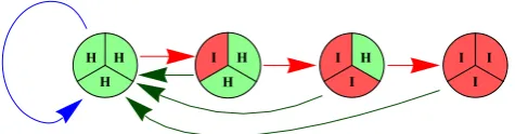
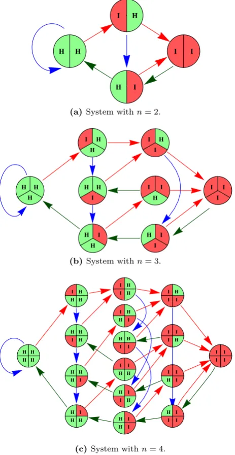
The diagram in Fig. 1a illustrates the possible states and state-transitions of a system with n=3. Note that the

(i+1)thleftmost column of circles contains all global states with exactlyiintruded nodes. Thus, a3, fsystem, for any

f <3, is failed whenever its global state corresponds to any

Fig. 1 State diagrams of intrusion for a system withn=3 nodes. In each sub-figure, eachcircle represents a global state of the system, with eachinner trianglerepresenting the state of a node: healthy (H) or intruded (I). Eacharrowrepresents a transition where a single node changes from H to I. Eacharrowcorresponds to a constantintrusion rate(λ)

circle to the right of the(f+1)thleftmost column. The dia-gram naturally suits the parallel attack model, if each arrow represents a constant IRλ(resulting from a constant IAE). However, it could also fit a sequential attack model if for each circle only one outbound arrow (does not matter which) is allowed to have a positive IR, i.e., if only one transition is possible.

The diagram in Fig.1b, which is actually a sub-diagram of the one in Fig.1a, naturally suits the representation of a particular choice of sequential attack, if one considers that: each position of inner triangle (inside a circle) represents a particular node; and each arrow has an associated con-stant IR (λ). Actually, while not considering rejuvenations, all paths of sequential attack leading to failure are equally efficient, i.e., the ordering in which nodes are attacked is ir-relevant. With some flexibility (and this will be important when interpreting more complex diagrams in the remainder of the paper), this diagram can also be interpreted as rep-resenting a parallel attack model, if: the(i+1)th leftmost circle stands for all possible states containing exactlyi in-truded nodes (see Fig.1a); and the respective outbound ar-row of each circle stands for(3−i)possible transitions from each imagined source state to the respective possible(3−i)

A note on diversity The assumptions made so far do not consider cases of exploitation ofcommon-mode vulnerabili-ties, capable of leading all nodes to immediate simultaneous intrusion. If this were to be possible, the discovery of a vul-nerability in a node could facilitate the intrusion of remain-ing healthy nodes (a dependence between intrusions that would favor the attacker). In practice, avoiding such vulner-abilities is a hard-to-solve problem. A common technique to mitigate the problem involves implementing intentional di-versityin the replication and rejuvenating process of nodes, on the dimensions that sustain the vectors of attack [16] that are likely to be exploited. It is not our goal to discuss the feasibility or effectiveness of such techniques—we simply focus on constructed examples that fit well the model of in-dependence of intrusions. However,we strongly emphasize that we are not simplifying as in making awish for added security, but rather to show that, even with probabilistic in-dependence of intrusions across nodes, dependability prop-erties might still be brought down by the intrusion-tolerant techniques(e.g., replication)whose application would typi-cally intend otherwise.

A note on dependence It is also worth mentioning a com-monly overlooked fact: although, from a defensive point of view, independence of intrusionsis better than a possibil-ity of simultaneous collective intrusion, it is not an opti-mal situation. As noted in [24], “better than independence can actually be attained”. Actually, there are two orthogo-nal axes of dependence: one refers to the probabilistic as-pect of intrusions (our model is indeed of independence, be-cause the ratio IR/IAE does not depend on the number of intruded nodes); another refers to architectural aspects of at-tack (e.g., in the parallel-atat-tack model nodes are atat-tacked independently of others, whereas in the sequential-attack model there is agood dependence in the (defensive) sense that each node under attack protects all remaining healthy nodes from being attacked).

Examples of potential attack scenarios We emphasize that it might not be within the reach of an attacker to decide freely about the characteristics of a possible attack to a sys-tem. For example, a goal of stealthiness may require a lim-itation of the IAE upon each node. Also, the architecture of the system might protect itself from exposure to a certain type of attack ( or ∴). Of course, each system might lend itself to differentvectors of attack, i.e., to several ways of having one or more vulnerabilities being exploited. The fol-lowing informal examples are consistent with our assump-tions and illustrate possible constraints on attacks:

– IAE limited to ensure stealthiness. Consider a set of online nodes, each protected with a random-one-time-password, under a -attack using random password at-tempts, with equal frequency in all nodes. If the system is

prepared to sound an alarm if too many incorrect passwords are attempted in a given window of time, then the attacker must limit its IAE in order to remain undetected. In this case, a -attack onnnodes cannot be replaced by a∴-attack with a focusedeffortntimes higher in a single node at a time.

–Parallel type required by architecture, IAE limited by reactiveness. Consider a server application with a certain buffer-overflow vulnerability, leading to immediate intru-sion if exploited with a certain code-injection. If an, f

system were to be built withnonline servers (nodes) with the same application, then an adversary could potentially in-trude all of them simultaneously (i.e., with the same code injection). To prevent such dependency, consider that an in-struction set randomization(ISR) mechanism [24] is used, where the server-application of each node corresponds to a randomized version, indexed by an independent small key. The ISR might not remove the vulnerability of each node, but simply obfuscate it, such that a different code injection, unknown in advance to the attacker, is necessary to pro-voke intrusion. The attacker might still intrude each node, by trial and error attempts until it guesses the respective randomization key, but the intrusion success is indepen-dent between nodes. The frequency of such attempts (and thus, proportionally, the IAE) might be limited if each un-successful buffer-overflow attempt makes the server crash and reboot. Additionally, let the communication between a client (the attacker) and a set of servers (the nodes) be me-diated by a proxy which, for each client-request, establishes a connection with a random server. In this example, the at-tacker is limited to a -attack, because, from a coarse time-granularity point of view, each server experiences the same average of intrusion attempts per amount of time (i.e., the same IAE).

– Sequential Attack due to attacker’s limitations. Con-sider a single-person (the attacker) that is well skilled in a type of social-engineering attack, requiring human physical presence for a continued amount of time. If the system be-ing targeted is a set of geographically dispersed nodes, then the individuality of the attacker only allows him to perform a∴-attack. For a similar type of example, consider an at-tack that requires a distinct learning phase for each node (e.g., learning a language). If each learning task is more effi-cient when performed in a focused way, then a∴-attack type might be preferable. For compatibility with Assumptions1 and2, each intrusion should not provide any advantage to the next intrusion, or, more precisely, the proportionality ra-tio between IAE and IR remains constant and the IAE itself remains constant.

proceed sequentially through the inner layers, then only a ∴-attack type can be performed.

In the next section, we shall compare how reliability is affected by different types of attack, among other varying parameters. We argue that it is pertinent to compare differ-ent models, because in practice the same system might be subject to different adversarial environments.

3 Time, reliability, resilience

In this section, we consider thereliability(R) ofn, f sys-tems, under each model of attack and in several perspec-tives:

1. Whichn, fsystems have adesirable expected time to failure(ETTF)?

2. For whichmission time(MT) does an, fsystem have adesirableR?

3. Given a MT, a goal ofRand a functional relation (e.g., a ratio) betweenreplication degreen andintrusion toler-ance thresholdf, how to adjustf orn?

4. How to define goals of R-improvement and how to achieve them?

To be practical, we shall group systems by functional relations n(f ) or f (n), relating the degree of replication (n) with the intrusion tolerance threshold (f). We shall use suggestive labels, such as Crash and Byzantine (in syn-chronous or asynchronous environment), to identify such groups. For example, simple Crash fault-tolerant systems are often achieved with n=f +1, i.e., f =n−1. It is also common to see Byzantine fault-tolerant systems with n=2f +1 or n=3f +1, i.e., f = (n−1)/2 or f = (n−1)/3. However, we emphasize that, de-spite the labeling, the analysis ahead will not be based on the type of faults, but only on the relation between n

andf.

3.1 Expected time to failure

For the reference system,1,0, the parallel ( ) and sequen-tial (∴) models of attack are equivalent. The probability of the single node becoming intruded follows an exponential distribution and the respective ETTF (μ1,0=1/λ) is the inverse of the node’s intrusion rate (IR) (λ) (see (3), (4), and (5) in theAppendix).

The ETTF is a metric often used to obtain a quick intu-ition about the reliance of a system in terms of time, e.g., about the duration of time for which the system should be trusted to hold some security property. Also, the MT of a system is often defined as a function of its ETTF. Thus, we now determine the circumstances in which the ETTF in-creases or dein-creases with the number of nodes (n). Letμn,f

stand for the ETTF of an, f system. By Definition5, a system has a desirable ETTF ifμn,f > μ1,0or, equivalently, when the ratioμn,f/μ1,0is higher than 1. We shall now ana-lyze this ratio for different families ofn, fconfigurations.

ETTF under parallel attack In this model, the ratio is

μn,f/μ1,0= n

i=n−f1/ i, as deduced in [25]. Intuitively,

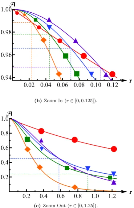
thef +1 terms in the sum correspond to thef +1 intru-sions that would lead to a failure. Figure2a shows curves for several cases, assuming a simultaneous unitary intru-sion adversarial effort(IAE) upon each node, i.e.,λj(t )=

1−φj(t ). In the extreme of higher ETTF is the type of

system ( ) that works correctly while at least one node is healthy (f =n−1), having a ratio of μn,n−1/μ1,0= n

i=11/ i (a sum withn terms). When theintrusion toler-ance thresholdratiof/ndecreases below a certain limit, the system eventually transitions to an undesirable ETTF. The Lim FT curve () illustrates, for several values of f, the limit case of desirable ETTF. Asymptotically (in the limit

n→ ∞), the transition occurs forf/n=(1−1/e)≈0.63, withe≈2.718 being Euler’s number. For lowerf/nratios, the global ETTF decreases while the thresholdf increases, as seen in curves withf =(n−1)/2 ( ) andf=(n−1)/3 ( ), typically used in Byzantine fault-tolerant (BFT) sys-tems. Though decreasing, for these cases the ETTF still con-verges to a positive value. For example, withf =(n−1)/3, the ETTF tends to log(3/2)≈40.5% ofμ1,0. In a further extreme, when the ratiof/nitself converges to 0, while in-creasingf, the ETTF also converges to 0, as shown with theSqrt FTcurve ( ), with n=f2+1. The lowest ETTF happens without intrusion tolerance, i.e.,f=0 (only illus-trated forn=1), for which the ETTF decreases inversely proportional ton, i.e.,μn,0/μ1,0=1/n.

ETTF under sequential attack In this model, the ETTF is much higher, with μn,f/μ1,0=f+1 (also deduced in [25]), if λis fixed when varying n. Each node has an ex-pected time to intrusionofμ1,0, out only when it starts be-ing attacked. The higher increase of ETTF withf is now the result of a (good) dependence between the IAE on different nodes. Intuitively, a node being attacked draws all the atten-tion from the attacker, and thus, while healthy, it protects the other nodes from being attacked. Figure 2b highlights the ETTF in function ofn, for differentf, nsystems. Note that, if this graphic was plotted in function off, all curves would superpose, asμn,f is now a pure function off. The

set of systems labeled asLim FT(b,) is printed just as a curiosity, as for a sequential attack they do not correspond to any interesting threshold. Thestrangerform of this curve is due to the nonmonotonicity of the ratiof/nfor the se-quence of plotted points (enablingf from 0 to 6)—note in

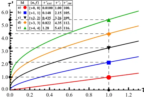
Fig. 2 Expected time to failure (ETTF) under attack. In each sub-figure, each point (a marker along a dashed line) indicates the ETTF (the position in the vertical axis) of a specific intrusion-tolerant systemn, f, withnbeing the total number of nodes andf being the threshold of tolerated intrusions. The marker represents the reference system1,0. Each other type of marker ( ,, , , ) represents a specific functional relation betweennandf(as detailed in the auxiliary box in the upper area of each sub-figure). The

vertical axis(labeled ETTF) actually measures the ratio

μn,f/μ1,0, between the ETTF of the respectiven, fsystem and the ETTF of1,0. For

λ=1, it follows that

μ1,0=1/λ=1, so the ratio is indeed the ETTF ofn, f. The

horizontal dashed line, starting to the right of marker , highlights the threshold between

desirableandundesirable

Fig. 3 Reliability (R) under parallel attack. The horizontal axis mea-sures the mission time (MT) τ in a scale normalized to the ETTF of the reference system 1,0, i.e., normalized toμ1,0=1/λ. For each curve, associated with a specificn, fconfiguration, the verti-cal axis measuresRn,f(τ ), and the respectiveτmax(in the rightmost

column of the auxiliary box on the upper right) is the value satisfying

τ∈ [0, τmax] ⇔Rh,f(τ )≥R1,0(τ )

In conclusion, the differences in types of attack ( versus ∴), may make the difference between improving or wors-ening the ETTF of a system, whenaugmentingits configu-ration from1,0 ton, f. This should bring to attention the importance of considering architectural aspects that may limit the types of attack, when deciding on how to achieve intrusion tolerance.

3.2 Reliability per mission time

The ETTF is a useful metric, but there is no fundamental reason for it to be the desired MT. Thus, we now consider a more dynamic perspective and analyze thereliability(R) for different MT values. We are interested in knowingwhat are the mission times for which intrusion-tolerant replica-tion does not worsen the reliability of a system, when com-pared to that of1,0. This information is important when one wants to define an adequate MT given an, fsystem, or, vice-versa, select the bestn, f system given a prede-termined MT.

Henceforth, symbolτ shall be used to express time nor-malized toμ1,0=1/λ, theexpected time to intrusion(ETTI) of a node under attack. When considering this unit, one can assumeμ1,0=1 (and consequentlyλ=1/μ1,0=1). Equiv-alently, whateverλ, one can assumeτ =t /μ1,0=λt, where

t is (the wall-clock) time used to measure 1/λ(recall thatλ

is a rate).

The analytic formulas forRin the -attack model and in the∴-attack model are given in theAppendix(see (9) and (13), respectively).

Reliability under parallel attack Figure 3 and Table 1 show the variation ofR_n,f(τ )for several pairsn, f. When

Fig. 4 Mission time (MT) for the same reliability as that of1,0, under sequential attack. Thehorizontal axismeasures the MT (τ) of the reference system1,0. Eachcurveis associated with anintrusion tolerance thresholdf, but is independent of thereplication degreen. Thevertical axismeasures another MT (τ), such that, if the curve associated withn, fincludes pointτ, τ, thenRn,f∴ (τ)=R∴1,0(τ ). Curvea( ), withf=0, is the identityτ=τ

asmallamount of time has passed, an intrusion-tolerant sys-tem withf >0 has desirableR , because it is not yet likely thatmanynodes have been intruded. As time passes, more nodes are likely to have been intruded, and thus a low ra-tiof/nmay imply lowerR . In Fig.3, we show solutions (τmax) of the MT for whichR transitions fromdesirable toundesirable. In other words,[0, τmax]is the interval for whichR_n,f(τ )≥R_1,0(τ ).

For example, consider a context that requiresn=3f+1 and for which each node under attack has an estimated expected time to intrusion of 1 year. In Table 1, we see that, when compared to 1,0, a system 4,1 has desir-able R for τ=0.2, i.e., a MT of 2.4 months, because R4,1(0.2) >R1,0(0.2). However, for τ=0.5, i.e., a MT of 6 months, the respective R is undesirable, because R4,1(0.5) <R1,0(0.5). In Fig.3, we see τ =0.264 as the transition value (τmax) of4,1.

Table 1 Reliability (R) under parallel attack. Each row corresponds to a differentn, fsystem. Each column (below the top merged cell labeledR) corresponds to a different MTτ, normalized to the ETTF of the reference system1,0. The values ofdesirablereliability (i.e., those that are higher than the reliability of1,0for the same MT) are highlighted in slightly larger font size

On a more global look to Fig. 3 and Table 1, we note that different functional relations between n andf imply different MT-ranges of desirableR :

1. any MT—e.g., theCrash FT curve, in representation of any curve withn=f +1, is higher than theReference curve for any positive MT;

2. MT up to someτmax>1—e.g., theLim FTcurve, in rep-resentation of any curve withn= _e−e₁f+1 andf ≥2, intersects theReferencecurve forτ >1;

3. MT up to someτmax<1—e.g., theBFTcurves, in rep-resentation of any curve withn=2f+1 orn=3f+1 (forf >0), intersect theReferencecurve forτ <1; 4. never—e.g., system2,0(see Table1), in representation

of any replicated but non-intrusion-tolerant system (i.e.,

n >1 andf =0), has lowerR than that of the Refer-ence, for any positive MT.

Reliability under sequential attack In this model, the time required to intrude more thanf nodes is independent of the total number of nodes (n). For any MT, the reliability al-ways grows with the intrusion tolerance threshold f (see (14). Still, for anyn, f system, reliability converges to 0 as time increases (see (14)).

For the sequential-attack model, a graphic equivalent to the one in Fig.3(i.e.,R∴versusτ) would have no curve in-tersections. Thus, we proceed directly to a new perspective, showing in Fig.4how an increase off allows an increase of MT, fromτ toτ, without changing theR∴of the overall system. Note that the ratioτ/τ is much smaller nearτ =1 than it is for smaller values ofτ. For example, a reference system1,0used for a MT ofτ =0.01 has the sameR∴ has an intrusion-tolerant system withf =4 used for a MT ofτ=1.28, i.e., 128 times higher. However, if the reference of comparison is1,0for a MT ofτ =1, then the replicated system withf =4 has higher reliability only when used up

to a MT ofτ=5.43, i.e., only 5.43 times higher. The solu-tion ofR∴_1,0(τ )=R∴_n,f(τ)in order ofτis presented in the Appendix(see (15)).

3.3 Time periods withrelative-resilience

It is easy to understand what it means to increase the MT by a multiplicative factor. However, withreliability (R), a probability, the scale is not linear and thus it may not be meaningful to ask for a linear improvement of R(e.g., to improveRby a factor of 2). Nonetheless, in the interest of intuition, we would like to be able to make comparisons in a linear scale, while still relating with the concept of reliabil-ity. To deal with this, we define a new metric, to which we suggestively callresilience(ρ), increasing linearly with the number of bits with whichRis close to 1.2In other words, improvingρby one unit means increasing theRby halving its distance to 1 (see (16) in theAppendix).

We can now make significant questions in a linear scale, such as: what are the values of mission time (MT) for which the resilience(ρ)of n, fis at leastctimes higher than that of 1,0 (see (17) and (18) in the Appendix). Note that we may talk about a relative-resilience im-provement brought upon by a n, f configuration, if

c >1, even though the absolute resilience (ρn,f(t ))

de-creases with time (i.e., with the increase of MT) for any n, f configuration. We emphasize that, consistently with the enunciated goals of this paper, this is an ob-jective way of measuring a dependability improvement brought upon by intrusion-tolerant replication in our system model.

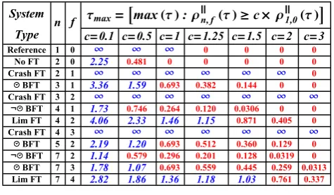
Resilience under parallel attack Table2presents some nu-merical solutions for the periods of MT for which an, f

system, under parallel attack ( ), should be designed for when intending a certain relative-resilience factor (c). Some interesting facts:

– Every n, f system has a maximum relative-resilience factor that it can sustain. Forn=f +1, any factor (c) is valid either for any MT (τmax= ∞) or for none at all (τmax=0). For the other illustrated systems, anyc >0 is valid only for a finite duration.

2_{This approach can be found in related areas. For example: the “nines} of availability” counts the nines in the decimal expansion of the value ofavailability(A); a cryptographic algorithm is sometimes said to

Table 2 Time Periods (τ) with relative-resilience (c) under parallel attack ( ). Each row corresponds to a differentn, fconfiguration. Each column (below the top merged cell definingτmax) corresponds to a specific relative-resilience factorc.τis a measure of time normal-ized to the ETTF of the reference system1,0, i.e., such thatμ1,0=1. Each cell, intersection of a column with valuecand a row with con-figurationn, f, contains the maximum mission time value (τmax) for which the relative-resilience of then, fconfiguration is at leastc. Valuesτmaxare highlighted in slightly larger font-size if the respective

cis valid forτup to at least 1

– With replication (i.e.,n >1) a lack of intrusion-tolerance (i.e.,f =0) always implies lower resilience, i.e., for any MT the relative-resilience is always lower than 1 (see (19) in theAppendix).

– For anyf≥1, someρ-improvements (i.e.,c >1) can be obtained for a small MT. However, only large ratiosf/n

allowρ-improvements for large MT.

As an example, consider a MT τmax=0.0319, as ob-tained in Table2forc=2 and7,2(a possible BFT system with configurationn=3f +1). Using (9) and (16) (in the Appendix), we calculate thereliability (R) and respective resilience(ρ):

– for1,0,R1,0(0.0319)≈96.9%⇒ρ≈5.0; – for7,2,R7,2(0.0319)≈99.9%⇒ρ≈10.0.

Thus, a system 7,2 is approximately 2 times (c≈

10.0/5.0 = 2) more resilient than the reference (non-replicated) system1,0, for a mission time oft≈0.0319×

μ1,0. Ifμ1,0(the ETTI of each node) is 1 year, then the (at least) double resilience is valid for a MT of about 11.4 days (0.0319×1 year).

Resilience under sequential attack Under sequential at-tack, the resilience increases with the intrusion tolerance thresholdf, as a consequence of the reliability also increas-ing. In Table3 we show some numerical solutions relating MT (τ) and relative-resilience factors (c), for several val-ues off. An interesting qualitative difference can be noted in comparison with the parallel attack model. In the sequen-tial model, even though the absolute resilience still decreases with the increase of time, the relative-resilience factor actu-ally increases with MT (thus Table3refers toτmin, instead ofτmax).

Table 3 Time periods (τ) with relative-resilience (c) under sequen-tial attack (∴). Each row corresponds to a different intrusion tolerance thresholdf, for which anyn, fsystem withn > f applies. Each column (below the top merged cell definingτmin) corresponds to a spe-cific relative-resilience factorc.τis a measure of time normalized to the ETTF of the reference system1,0, i.e., such thatμ1,0=1. Each cell, intersection of a column with valuecand a row with valuef, con-tains the minimum mission time (τmin) for which the relative-resilience of then, fconfiguration is at leastc. 0+indicates that any posi-tive value of mission time satisfies the condition of relaposi-tive-resilience higher thanc(note that the comparison operation is>and not≥, so thatτmin is not trivially 0 for anyc). Valuesτminare highlighted in slightly larger font-size if the respectivecstarts before someτsmaller than 1.τminis 0+wheneverc≤f+1

4 Availability and the role of rejuvenations

In this section, we analyze the dependability enhancement brought upon by the use ofproactive rejuvenation[6,18, 22].Rejuvenation is a process that restores the state of a node tohealthy, regardless of its previous state. Consistently with our model of intrusions and attacks (Assumptions1 and2), we assume that the eventual intrusion of a node, at a given time, does not make easier the future intrusion of other nodes, not even of the same node after rejuvenation. This type of independence is usually achieved by the use ofdiversity, which might be effective for certain vectors of attack. Within our scope, we keep agnostic to the implemen-tation of diversity, simply assuming that it might be effective in some cases of practical interest, and thus we measure de-pendability in a conservative way.

Fig. 5 Timeline of different Rejuvenation Models. In each sub-figure, time flows in the horizontal axis from left to right, starting att=0. Eachrowrepresents the timeline of one of thennodes in a system. Theempty slotsstand for online time; theslots with letter R inside

stand for (offline) rejuvenation time. In each column, there are exactly

n−knodes online andknodes rejuvenating. Thethicker vertical seg-mentsmark the beginning and ending instants of each rejuvenation, either as an instantaneous process (r=0) whenk=0 (sub-figures5a

and5b), or as a process taking some time (r >0) whenk >0 (sub-figures5c and5d). The auxiliarysmall circles, on top of some thick vertical segments, examplify the horizontal extremities of the measure of some parameter of the rejuvenation scheme (as respectively exem-plified below the lowest timeline row):r is the time a node takes in each rejuvenation;Δis the period between the beginning of consecu-tive rejuvenations of the same node;δis the minimum time between rejuvenations of different nodes

4.1 Extended system model

If we could detect attacks and/or intrusions, then areactive rejuvenationscheme could be implemented [21]. For exam-ple: a detected attack could be mitigated by rejuvenating components more frequently; a detected intrusion could be amended by immediately rejuvenating the respective node. However, in our context of stealthiness, we can rely only on proactive rejuvenation schemes, of which we shall describe two models:parallel( ) andsequential(∴).

Assumption3formalizes both types of rejuvenation and Fig.5illustrates the timeline of node rejuvenations for sev-eral specific rejuvenation schemes.

Assumption 3 (Periodic Rejuvenations) Let n >0 be the total number of nodes in a system that initiates its oper-ation at instant 0. At any instant of time t >0, let k∈

{0, . . . , n−1}be the constant number of rejuvenating (of-fline) nodes and let n=n−k be the number of online nodes. LetΔ >0 be the (periodic) interval of time between the beginning of rejuvenations of the same node. Letδ(with 0≤δ < Δ) be the smallest time between the beginning of rejuvenations of different nodes (δis equal to 0 if different nodes rejuvenate simultaneously). Letr≥0 be the time

du-ration of each rejuvenation of any node. Nodes 1 through

n become online for the first time simultaneously at in-stant 0. Forj ∈ {n+1, . . . , n}, nodej becomes online for the first time at instant(n−j +1)×δ; before that it is considered to be in its 0threjuvenation. Forj ∈ {1, . . . , n}, nodej begins itsithrejuvenation(withi∈N1), at instant

(n−j +1)×δ+(i− [j ≤n]?)×Δ, where [j ≤n]?

is 1 if j ≤n and 0 otherwise. Moreover, k is a constant integer satisfyingr=δ×kandr=Δ×(k/n). Rejuvena-tion schemes are distinguished in two types:parallel( ), if

δ=0, orsequential(∴) otherwise. A system without reju-venation is denoted as a -rejuvenating system withΔ= ∞.

Figure5illustrates clearly some differences between the timelines of distinct types of rejuvenations ( and∴) and dif-ferent number of simultaneous rejuvenating nodes (k). For parallel rejuvenations (Fig. 5a): nodes rejuvenate simulta-neously (δ=0) after every interval ofΔtime units; since (by assumption) the duration of rejuvenation of each node is proportional toδ, if follows that rejuvenations are instan-taneous3 (r=δ×k=0) and thus nodes are never offline

instanta-Fig. 6 State diagram of a rejuvenating system withn=1 node, under attack. Each circle represents the state of the single node:healthy(H) orintruded(I). A rejuvenationheals(H HorI→H) the node. An intrusionintrudes(H I) the node

for a continuous amount of time (i.e.,k=0). For sequential rejuvenations, nodes can also rejuvenate instantaneously, if

k=0 (Fig.5b), but each one does so at a different instant in time (i.e.,δ >0); ifk=1 (Fig.5c) then once a node be-comes online another one immediately starts rejuvenating; finally, ifk >1 (Fig.5d), then several nodes can be in re-juvenating state simultaneously, but starting at different in-stants of time. In any case, each node isonlinefor durations of Δ−r, interleaved with offline durations of r, and the number ofonlinenodes is a constant (n=n−k).

Extended model By combining the models of attack, in-trusion, and rejuvenation, we get an extended model where healthy nodes can be intruded and then be reverted back to a healthy state. In this new system model,naccounts also withkoffline nodes. In typical systems, the parametersn,f

andkare related in a linear way, i.e., asn=af+bk+c, for non-negative integersa, b, andc. For simplicity, we shall restrict the remaining comparison examples to cases with

b=1 andc=1. Thus, a tripletn, f, kwill henceforth be used, to denote the full constitution of the system in terms of numbers of nodes (an exception is made to the reference systemn, f = 1,0, which clearly impliesk=0). We as-sume that attacks can influence the rate of state transitions (as determined in Assumption1), but cannot influence the schedule of rejuvenations.

For each n, f, k system, the rejuvenation duration (r) of a node is related with the periodicity of rejuvenations by

r=Δ×(k/n)or r=δ×k, respectively for rejuvenations of type or ∴. Thus, we may characterize a system with only two extra parameters in subscript:

– , Δ:parallel( ) rejuvenations with periodΔ, and as-sumingδ=0.

neous rejuvenations by considering the existence of virtual nodes ( vir-tualin the sense of never being online, and not being accounted in parametern), whose role is only to help preparing the future instan-taneous rejuvenation ofrealnodes. In that case we shall still refer to instantaneous rejuvenations, even thoughrwill be considered as a pos-itive value given byr=Δ×(k+vk)/n, wherevkis the number of virtual nodes.

Fig. 7 State diagram for parallel rejuvenation of a system withn=3 nodes, under a particular choice of sequential attack. Eachcircle repre-sents the set of 3 nodes and their states. For parallel rejuvenations, the order in which nodes are intruded is irrelevant, and only the number of intruded nodes matter. Thus, a more general interpretation (suitable also for the case of parallel attack), considers that each circle withi

triangles in stateIis representative of all global states with exactlyi

nodes intruded

– ∴, δ: sequential (∴) rejuvenations, with consecutive nodes being rejuvenated at instants separated byδ, and withΔ=n×δ.

In terms of parameters characterizing the external envi-ronment, we shall continue to use or ∴ for the type of attack (parallel or sequential) andλfor theintrusion adver-sarial effort(IAE) upon each node.

Types of rejuvenation The choice of rejuvenation type might not be arbitrary. By assuming a scenario of stealth attacks and intrusions, proactive rejuvenations must be im-plemented with a protocol that is resilient to intruded nodes, even though they might be indistinguishable from healthy ones. For example, if the system implements non-stop op-erations, the rejuvenation process might require transfer of state from online nodes to rejuvenating nodes, thus making asequential rejuvenation scheme more appropriate than a parallelone. In such cases, parameterskandrare relevant in terms of implementation. Actually, an eventual inability to enforce a fixed bounded limit onrmay result in security vulnerabilities for some protocols, as noted in [22].

The 2 models of attack and 2 models of rejuvenation give 4 possible types of combinations. However, for a sys-tem made of a single node (n=1) all combinations collapse into the same model—Fig.6shows the respective state di-agram. Notably, for the reference system1,0(or actually any other withf =0),rejuvenationdoes not affect reliabi-lity(R), because: (1) theintrusionof a node corresponds to the immediate failure of the system; and (2) the rejuvena-tion of a healthy node does not alter itsintrusion rate(IR). Consequently, if there is no intrusion tolerance then a R-improvement can only be obtained by using more reliable nodes. Nevertheless, availability (A) is improved with reju-venation even for the reference case withn=1. Forn >1, we analyze the models separately.

4.2 Parallel rejuvenation

state, i.e., with all nodes healthy (see (20) in theAppendix). As an example, Fig.7shows the state diagram for a system withn=3 and k=0, subject to parallel rejuvenations. In comparison with Fig.1b, only the rejuvenation transitions were added.

In the parallel rejuvenation model, the overall reliabil-ityas a function of time(Rn,f, ,Δ(t ))can be obtained as a

product ofreliabilities (Rn,f) for time-windows of width

Δ(i.e.Rn,f(Δ)) and less (i.e.Rn,f(m)for somem < Δ)

(see (21) in theAppendix). Forn, fsystems withf >0, rejuvenation might healintrudednodes before the number of simultaneous intrusions exceedsf. Recalling Fig.3, we conclude that intrusion-tolerant replication and rejuvenation may have complementary roles in dependability:

– intrusion-tolerant replication, with f >0, improves R for small MT, but for small ratios f/n it is prejudicial for large MT;

– rejuvenationcannot bring benefits before its first applica-tion,butit reduces the long-term degradation effects on dependability, by periodically bringing the system back to its initial overall state (i.e., with all nodes healthy—see (20) in the Appendix).

By applying both techniques together (rejuvenation and intrusion-tolerant replication), theRimprovement might be valid even for an unbounded MT (finite but not known in advance). To achieve such overall improvement, an, f ,Δ

system must have a low enough periodΔ, namely less than the threshold value of time (in Fig.3) for whichn, f (with-out rejuvenation) transitions toundesirableR. In this way, even configurations 3,1 and 4,1 under parallel-attack may havedesirableR. This amends the negative result (for dependability) that we had achieved with the preliminary system model. However, ifMT = ∞thenRn,f, ,Δis

sim-ply 0, whereas An,f, ,Δ is still positive (see (22) in the Appendix).

4.3 Sequential rejuvenation

A more challenging analysis is that of sequential rejuvena-tions, for which there is no periodic interval for which the overall system state is reset, even though the instants of juvenation are periodic. This happens because nodes are re-juvenated one at a time, thus not guaranteeing that the num-ber of intruded nodes goes back to 0. In particular, a strong-enough attacker may be able (probabilistically) to intrude nodes at a faster pace than their rejuvenation. As a conse-quence, the number of intruded nodes may potentially be maintained above the thresholdf for durations much longer thanδ×n. Moreover, for a sequential-attack there are paths of attack with different effectivenesses, because of their re-lation with the ordering of rejuvenations. In this respect,we always assume an optimal IAE sequence, from the point of view of the attacker, as stated in Assumption4.

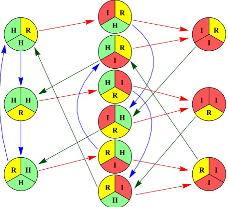
Fig. 8 State diagram of sequential rejuvenation of a system withn=3 andk=1, under optimal (i.e., most effective) sequential attack. Each

circlerepresents a set ofn=3 nodes and their states:healthy(H), in-truded(I) orrejuvenating(R). The types of transition are illustrated with arrows with different directions:rightward, when a previously healthy node transitions to intruded state;leftward, when a previously intruded node transitions to rejuvenating state;vertical(downwardor

upward), when a previously healthy node starts being rejuvenated

Assumption 4(Optimal IAE sequence) Under sequential rejuvenation, a sequential attack always targets the (yet) healthy node which will remain un-rejuvenated for the longest time.

State diagrams showing rejuvenations Figure 8 shows a state diagram for a system withn=3 andk=1, where there are always 2 online nodes and 1 rejuvenating (offline) node. Some transitions triggered by rejuvenation occur between circles in the same column, as they correspond to the start-ing of rejuvenation of a previously healthy node, thus keep-ing constant the number of intruded nodes. Also, given our assumption of an optimal attack sequence, each circle of the leftmost column has only one outbound arrow correspond-ing to intrusion, leadcorrespond-ing to a circle in the middle column for which the next rejuvenation will not reduce the number of intrusions. In this diagram there are cycles that never go back to a completely healthy state, contrarily to what would happen in a diagram for parallel rejuvenations (e.g., Fig.7).

Fig. 9 State diagrams of sequential rejuvenations withk=0, under optimal sequential attack. Each sub-figure depicts the state diagram of a system with a different number of nodes (n∈ {2,3,4}). In each sub-figure, each circle represents a set ofnnodes and their states:

healthy(H) orintruded(I). A rejuvenationheals(H H orI H) the right-upper triangle and then rotates the circle counter-clock-wise by 2π/n(i.e., by 1/nof a full circle rotation). An intrusionintrudes

(H I) the healthy triangle further away (in time) being healed

the rejuvenating node of 3, f,1, we are left with a sys-tem of only two nodes, i.e.,2, f,0, as shown in Fig.9a. In other words, Fig.8can be mapped onto Fig.9a, by map-ping each 3 circles and 3 arrows onto an equivalent single circle and arrow, in the same column. Henceforth, we shall use these simplified diagrams that hide the complexity of rejuvenating nodes. Also, when making simulations to de-termine the availability of systems with sequential

rejuve-nation, we shall actually simulate n−k, f,0 instead of n, f, k, which is equivalent, after doing the necessary ad-justments to the valuesrandΔ.

Consider in Fig.9a the rejuvenating transition from (I|H) to (H|I), represented by the downward arrow ( ) in the mid-dle. Note that, despite the flipping of positions of letters I and H, the same nodes remain intruded and healthy. What changes is the time-distance that the intruded node is away from its future rejuvenation. The transition corresponds to moving from a state witha single intruded node being two rejuvenating-steps way from healing, to a state withthe same intruded node being only one step away from healing. In other words, the transition corresponds to the case where the rejuvenation is applied to a healthy node, thus not alter-ing the number of intruded nodes of the system, but bralter-ingalter-ing the intruded node one step closer (in time) to being rejuve-nated (i.e., it will be healed in the next rejuvenating step). Also, note that from the leftmost column to the middle col-umn only one intrusion arrow exists—the arrow ( ) going from (H|H) to (I|H). This is consistent with Assumption4, under which a sequential attack always targets the healthy node that is further away from rejuvenation.

We have seen how to go from Fig.8to Fig.9a. Following the same logic, we can simplify the analysis of sequential-rejuvenating systems with non-instantaneous rejuvenations (i.e., with k >0) for other values of n. To simplify, we shall look instead to the system withn=n−knodes and

k=0 offline nodes at any time (and consequently with in-stantaneous rejuvenations). In the remainder of this section, we shall compare differentn, f, ksystems, the biggest of which being4,1,1(i.e.,n=2f+k+1, withf =1 and

k=1) and 5,1,1(i.e.,n=3f +k+1, withf =1 and

k=1). Their respective equivalent diagrams are depicted in Fig.9b (n=3 andk=0) and Fig.9c (n=4 andk=0).

The rules of probabilistic transition between states are easy to define and simulate. As an example, Fig.10shows results of availability (A) for a parallel attack model (sub-figure10a) and for sequential attack model (sub-figure10b), when varying δ (the offset between sequential rejuvena-tions). We consider cases withk=1, and thus δ=r. Let

n=n−k. The curves shows that differentn, fsystems havedesirable A(i.e., higher than that ofn, f = 1,0) for different offsetsδof rejuvenations: for anyδifn, f =

2,1; only for δ0.10 or δ 0.26, if n, f = 3,1, under or ∴ attack, respectively; only for δ 0.024 or

δ0.11 ifn, f = 4,1, under or∴attack, respectively. 4.4 A practical comparison of configurations

Fig. 10 Availability (A) with sequential rejuvenations. Each sub-figure corresponds to an environment under a particular type of attack: parallel ( ) in sub-figure10a; sequential (∴) in sub-figure10b. In each sub-figure: each curve corresponds to an, f, ksystem, wherenis the total number of nodes,fis the threshold of tolerable intrusions, andk

is the number of rejuvenating (offline) nodes at any given instant; the horizontal axis measuresδ, the time offset between rejuvenations of different nodes; the vertical axis measuresA, the expected proportion of time for which the number of intruded nodes is at mostf; in the

rightmost column of the auxiliary box in the upper right corner of each sub-figure, each valueδmaxis the maximum value of parameterδfor which theAof the respectiven, f, ksystem is better (i.e., higher) than that of the reference system (curve e, ); the reference curve was obtained from the analytical expression(1−er)/r; all other curves (i.e., for systems withf >1) were obtained by joining pairs(δ,A )

or(δ,A∴), withδspaced in intervals of at most 0.01, and withA or A∴_{, respectively, being an average over the result of 100 probabilistic} simulations with amission timeδ×105

that an intrusion-tolerant system must be built, subject to the following constraints:

1. the underlying protocol requiresn=2f+k+1, e.g., a typical synchronous or stateless BFT system with rejuve-nation (e.g., [21]);

2. resources are limited to a maximum of 4 nodes;

3. considering two possibilities of implementation, the sys-tem may either be attacked sequentially with a focused IAE ofλ=3 per node, or in parallel with a dispersed IAE ofλ=3/(n−k)per online node;

4. the rate at which nodes can rejuvenate is proportional to the number of available offline nodes, e.g., new (diversi-fied) software replicas are generated using the computa-tional resources of nodes that are not online.

With these restrictions,what is the configuration that en-ables a higherA, for an infinite MT?

Making a fair comparison The instantaneous rejuvenation (r=0) of nodes, in the case of parallel rejuvenations, still seems somewhat far-fetched. To substantiate it, we allow the existence of offlinevirtual nodes(vk), helping in the prepa-ration of new replicas. We characterize them asvirtual be-cause they are not to be accounted in the valuen(the total number ofrealnodes) as defined in Assumption3. However, for the purpose of this example, we make the virtual nodes count toward the limit of 4 nodes, i.e.,n+vk=4. To com-pare different systems in an equal standing, we require that a virtual node must work for timer in order to prepare the

instantaneous rejuvenation of a real node, whereris the ex-act same time that a (real) offline node takes to rejuvenate in a sequential rejuvenating scheme. Thus, we are now ready to consider the above question for different values ofr.

Comparable scenarios Considering the restrictions and the guidelines for fair comparison just stated, we shall com-pare 5 different scenarios:

• Single node case:The reference system is characterized by a single node online at any time, i.e., n−k =1. In this case, both parallel and sequential attacks are the same, and so we set λ=3, in accordance to the above guidelines. Also in this case, both rejuvenating schemes are equivalent, and so we can choose arbitrarily be-tween two notations. If seeing it as a ∴ rejuvenating scheme, thenn, f, k, vk = 4,0,3,0andrej, δ, Δ =

∴, r/3, (4/3)r andλ=3. If seeing it as a rejuvenat-ing scheme, thenn, f, k,vk = 1,0,0,3,rej, δ, Δ =

,0, r/3andλ=3.

• Two sequential-rejuvenation cases, withf >0:The con-figuration of nodes is limited ton, f, k,vk = 4,1,1,0; defining the time parameters in terms of r we get rej, δ, Δ = ∴, r,4r. Finally, there are two distinct vari-ants of this scenario: λ=1 for -attack; λ=3 for ∴-attack.

Fig. 11 Availability (A) in function of rejuvenation time(r)per node. Curves a) ( ), b) () and c) ( ) were obtained from the respective an-alytic expressions of availability; the curves of sequential rejuvenation cases, were obtained by joining pairsr,A, withrspaced in intervals of at most 0.01, and withAbeing an average over the result of 100 probabilistic simulations with a mission timeδ×105

ofr.rej, δ, Δ = ,0,3r. This case also has two dif-ferent variants, depending on the attack type:λ=1 for

-attack;λ=3 for∴-attack.

For any of the 5 cases under comparison (see Fig.11a): – at any given time, there are:n−kreal nodes online;kreal

nodes rejuvenating;vk extra virtual nodes helping with the preparation of rejuvenations;

– the global rejuvenation period (i.e., the time between two rejuvenations of the same node) isΔ=r×n/(k+vk); – the minimum time between rejuvenations of different

nodes is δ=r/ k for ∴-rejuvenations, and δ=0 for -rejuvenations;

– the sum of IAE across all healthy nodes is at most 3, i.e.,

n

j=1λj(t )≤3—in particular, for a -attack it is

propor-tional to the number of healthy nodes, and for a∴it is constant while there is at least one healthy node.

In Fig. 11, we plot the availability of such systems, in function of parameterr (time required to recover each node). This figure shows interesting results:

1. For each rejuvenation type, a focused∴-attack (λ=3) is more effective than a dispersed -attack (λ=1). This was expected given that for the -attack the sum of IAE (across all nodes) decreases with the number of healthy nodes. Moreover, when in∴-rejuvenations, the∴-attack is more effective by pursuing an optimal IAE sequence.

2. For each attack type, and withf =1, asrgrows, the availability of ∴-rejuvenations eventually becomes lower than that of -rejuvenations—see Fig. 11b or Fig. 11c for curveb() versus curved( ); see Fig.11c for curvec( ) versus curvee ( ). This was expected, as ∴-rejuvenations cannot guarantee a periodic complete recovery. Thus, a fast enough intrusion of nodes (or, equivalently, a slow enough rejuvenation of nodes) may keep the system failed for a long time. Yet, it is interesting to see that, in the sole case of -attack, the ∴-rejuvenation is more effective than the -rejuvenation ifr <0.58. Our intuition is that this happens because, for a strong -attack (or equivalently, for a low enough r), a ∴-rejuvenation allows a higher frequency of healing of eventually intruded nodes. This qualitative com-parison between rejuvenation types does not hold for ∴-attacks, because theoptimal IAE sequencetargets first the nodes that are further always from rejuvenation.

3. Asrgrows, the system with lowest intrusion tolerance threshold (f =0) but higher rejuvenation rate (i.e., lower

Δ/r) eventually becomes more available than the alterna-tives. This means that, if single nodes cannot be rejuvenated quickly enough, then it is better to increasekthanf.

5 Related work