C L I M A T E C H A N G E
Climate change in Latin America and the Caribbean:
policy options and research priorities
Brian Feld1•Sebastian Galiani2
Published online: 11 November 2015
The Author(s) 2015. This article is published with open access at Springerlink.com
Abstract Although climate change is filled with uncertainties, a broad set of
policies proposed to address this issue can be grouped in two categories: mitigation and adaptation. Developed countries that are better prepared to cope with climate change have stressed the importance of mitigation, which ideally requires a global agreement that is still lacking. This paper uses a theoretical framework to argue that in the absence of a binding international agreement on mitigation, Latin America should focus mainly on adaptation to cope with the consequences of climate change. This is not a recommendation that such economies indulge in free-riding. Instead, it is based on cost–benefit considerations, all else being equal. Only in the presence of a global binding agreement can the region hope to exploit its comparative advantage in the conservation and management of forests, which are a large carbon sink. The decision of which policies to implement should depend on the results of a thorough cost–benefit analysis of competing projects, yet very little is known or has been carried out in this area to date. Research should be directed toward cost–benefit analysis of alternative climate change policies. Policymakers should compare other investments that are also pressing in the region, such as interventions to reduce water and air pollution, and determine which will render the greatest benefits.
Keywords Climate change AdaptationCost–benefit analysis
JEL Classification Q52Q54
& Sebastian Galiani galiani@econ.umd.edu 1
Department of Economics, University of Illinois at Urbana–Champaign, Urbana, USA 2 Department of Economics, University of Maryland and NBER, 3105 Tydings Hall,
1 Introduction
Global warming is a particularly thorny externality because it is global and its effects extend for many decades into the future. To complicate matters even more, it has heterogeneous effects around the world. It requires a level of effort and commitment from the international community that is unparalleled in history, its consequences are potentially disastrous, and it is plagued with uncertainties.
While the physical mechanism that links greenhouse gases to global warming is clear and records show that the concentration of greenhouse gases has been increasing in the atmosphere for the last two centuries, a long list of scientific uncertainties makes it difficult to assess precisely how much warming will result from a given increase in greenhouse gas concentrations, when such warming will occur, or how it will affect different regions and ecosystems.
To address these concerns, the United Nations and the World Meteorological Organization established an international body—the Intergovernmental Panel on Climate Change (IPCC)—to assess the scientific knowledge on climate change. Projecting future climate trends is a complex endeavor. To cope with these complexities, the IPCC produced a set of emissions scenarios. Each scenario provides an alternative and internally consistent picture of how world development might shape future emission trends. Taking into account these scenarios, along with uncertainty about emissions and climate-system response, projected twenty-first century warming ranges from 1.1 to 6.4C (IPCC2007). Thus, while the magnitude of global warming that might occur in the future is indeed highly uncertain, all these scenarios agree on its upward direction.
Just as the effects of global warming on the climate system are uncertain, the physical and socioeconomic implications of climate change are not fully understood. Thus, uncertain physical risks are compounded by uncertain natural and socioeconomic consequences. Uncertainty about the effects of climate change and how to cope with them is also compounded by uncertainty about its cost. Costs are unknown due to possible changes in the available technology, the existence of irreversibilities in some policies that cope with the problem, and the presence of nonmarket goods and services that are vulnerable to climate change. In short, uncertainty is the single most important attribute of climate change as a policy problem.
A central concept in analyzing the effects of climate change is whether a system can be managed. The nonagricultural sectors of high-income countries are highly managed and this feature will allow them to better adapt to climate change. However, human and natural systems that are unmanaged or unmanageable are highly vulnerable. These systems include rain-fed agriculture, seasonal snow packs, coastal communities, river runoffs, and natural ecosystems. Thus, the potential damage of climate change is likely to be most heavily concentrated in low-income and tropical regions such as tropical Africa, Latin America, coastal states, and the Indian subcontinent.
a process is an externality that occurs because those who produce the emissions do not pay for that privilege, and those who are harmed are not compensated. One major lesson from economics is that unregulated markets cannot efficiently deal with harmful externalities. Any solution needs substantial reductions in the emissions of CO2into the atmosphere. An obvious instrument to achieve that goal is
to raise the market price of those emissions. Raising the price on carbon will achieve four goals. First, it will provide signals to consumers to reduce the consumption of goods and services that are carbon-intensive. Second, it will provide signals to producers to substitute away from inputs that are carbon-intensive. Third, it will provide market incentives to innovate and adopt new low-carbon products and process. Fourth, a carbon price will economize on the information that is required to undertake all these tasks (Nordhaus2008).
Rapid technological change in the energy sector is central to the transition to a low-carbon economy. Current low-carbon technologies cannot substitute for fossil fuels without a substantial economic penalty on carbon emissions. Developing economical low-carbon technologies will lower the cost of achieving climate goals. Therefore, governments and the private sector must intensively pursue low-carbon or even noncarbon technologies.
There are, of course, other actions that can be taken to manage the problem of global warming. Some of these actions are best performed by governments, while others are best undertaken by private agents acting on their own, such as adapting production practices to a changed climate. A general typology classifies these actions into mitigation and adaptation. Mitigation focuses directly on reducing the amount of greenhouse gases released into the atmosphere (thus assuming that human activity is partly responsible for the issue), while adaptation deals with increasing resilience to the consequences of climate change.
Developed countries, which are better prepared to cope with climate change, have stressed the importance of mitigation in order to limit temperatures to a range between 2 and 3C above preindustrial levels depending upon costs, participation rates, and discounting. Achieving such an objective will require a mitigation effort that is global in scope. International agreements should provide incentives to encourage participation, but the cost of those incentives should also be taken into account. To date there are no such agreements.
The next section of the paper describes the projected trends in climate change and what has been suggested to overcome them. Section3 then presents a list of available policies that have been proposed to address climate change, divided into three broad categories: adaptation, mitigation, and development policies that increase countries’ adaptive capacity. Section4 presents a theoretical framework, and Sect.5 provides a framework for evaluating different policies by their cost-effectiveness so that policymakers can efficiently choose the ones that should be implemented. Section6looks at the agricultural sector, an unmanaged system that has long been assumed to be able to adapt autonomously, while Sect.7 will concentrate on forestry, a sector on which the region should focus in the event that appropriate incentives for emissions reduction are put in place. The final section summarizes and draws conclusions in order to propose the direction for future research.
2 Global warming and its potential effects
According to various sources (IPCC2007; NOAA2012; NASA2012), the average global temperature has increased nearly 1C since data started to be systematically recorded in 1880. Despite the huge differences across regions, the upward trend has affected the entire planet. Working Group II of the IPCC Fourth Assessment Report compiled more than 500 studies that support these figures, and stresses that average global warming accelerated between 1970 and 2004, and that since then the slope has become flat (2007). Most of these studies concluded that global warming has affected physical as well as biological systems. In Latin America, different studies point to an average increase of mean surface temperature of nearly 0.10C per decade during the last century, but studies that focus on the second half of the century find an even higher increase per decade (IPCC2007).
One may thus wonder what could have caused this trend. Unfortunately, the exact causes and their relative contribution to global warming are not yet fully understood. Uncertainty over global warming is the rule rather than the exception, although the ‘‘greenhouse effect’’ was documented as early as the nineteenth century by physicist John Tyndall. Some gases in the atmosphere prevent heat from escaping into space, keeping the earth warm. The most prominent greenhouse gas in the atmosphere is water vapor, but it is followed by carbon dioxide (CO2), a byproduct of fossil-fuel
despite average global temperature showing a clear upward trend during the second half of the twentieth century, in the last decade temperatures have stabilized, although at record levels (NOAA2012). At the same time, the amount of greenhouse gases (particularly CO2concentration in the atmosphere) has never stopped rising
and is at now at record highs (Scripps Institution of Oceanography2015) . Scientists have not yet been able to explain this phenomenon, although possible explanations being investigated include a greater concentration of ash from volcanic eruptions and reduced levels of solar activity.
Uncertainty is exacerbated when we move one step further and try to assess the projected effects of climate change on the environment and the economy. First, projecting future scenarios using climatic models that include greenhouse gas emissions involves making assumptions in relation to population and economic growth and technological change, among other factors. Second, the mechanisms through which global warming will affect the environment are still subject to controversy, and this controversy expands as scientists collect more information and discover new ‘‘unknown unknowns’’ that could affect or be affected by global warming (Victor2011).
Despite all the uncertainty, however, there is scientific consensus that the upward trend in global temperature will prevail. If this is correct, then moderate (but not extreme) warming would actually bring global net benefits, although unevenly distributed: while countries at higher latitudes are expected to benefit, those closer to the equator will be worse off. However, researchers believe that warming beyond 2C will be costly in the aggregate (IPCC2007).
Temperature increases are reducing and may continue to reduce glaciers, producing many different adverse effects. A modest rate of ice-sheet melting (mainly in Greenland and West Antarctica) is expected to accelerate the pace of rises in sea levels reaching 2.2 m by the end of the century. Thus, low-lying and coastal areas (where about a fifth of the world population lives) will be at increased risk. Moreover, a reduction of inter-tropical glaciers is expected in the Andean region during this century. This may increase river flow in the short run, but reduce water availability in the long run and change the availability of water throughout the year, probably affecting energy supply. This has already been evidenced in Bolivia, Peru, Colombia, and Ecuador.
The effect on energy requirements is nevertheless uncertain. If temperatures rise, less energy for heating will be needed, but higher cooling consumption should be expected. This would produce a shift from fossil fuels to electricity, but the net effect will depend on each country’s energy sources.
The overall effects of global warming on agriculture are uncertain. According to the IPCC Fourth Assessment Report, food production will increase if temperatures rise from 1 to 3C because infertile, high-latitude lands (mainly in Canada, northern Europe, and Russia) will become productive. The increased amount of CO2in the
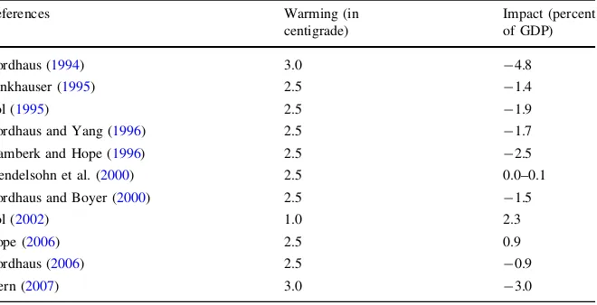
If estimating how global warming could impact natural and social environments is troublesome, costing these effects is even more difficult. The way to cost nonmarket goods—such as damage to or disappearance of ecosystem services, and loss of species or human lives—has not yet been agreed upon. Table1presents a list of studies carried out during the last two decades on the costing issue.
The available estimates of surface air temperature in the literature are similar among them because they are based on climatic models that expect the concentration of greenhouse gases in the atmosphere to double by the end of the century. In contrast, impact estimates (which reflect the yearly income reduction for the estimated temperature increase) vary greatly from one study to another, and even within studies carried out by the same researcher, because they are obtained using a variety of approaches and including a different number of sectors.
With the exception of Mendelsohn et al. (2000) and Nordhaus (2006), all the other studies use the ‘‘enumerative method’’ to estimate the effects of global warming. This means that physical effects are obtained from other disciplines (mainly natural science) that use climate and impact models, as well as laboratory experiments. For example, researchers use agronomy papers to estimate the impact of climate on crop yields, and then put a price on those effects using market prices or economic models. This is the case for every market good and service that is expected to be sensitive to climate change. For nonmarket goods and services (such as health), pricing comes from the valuation of those same goods and services in contexts different from climate change. As an example, suppose researchers assume that a natural reserve will disappear as a consequence of climate change. A reserve may have a recreational as well as an environmental value (absorption of CO2,
shelter for animals, etc.), but this value may be difficult and/or expensive to estimate. In order to do so, researchers use the cost estimates obtained from a study in which the source of variation in a reserve similar to the one under study is not climate.
Table 1 Estimates of global warming and its impact in terms of share of income lost
References Warming (in
centigrade)
Impact (percent of GDP)
Nordhaus (1994) 3.0 -4.8
Fankhauser (1995) 2.5 -1.4
Tol (1995) 2.5 -1.9
Nordhaus and Yang (1996) 2.5 -1.7
Plamberk and Hope (1996) 2.5 -2.5
Mendelsohn et al. (2000) 2.5 0.0–0.1
Nordhaus and Boyer (2000) 2.5 -1.5
Tol (2002) 1.0 2.3
Hope (2006) 2.5 0.9
Nordhaus (2006) 2.5 -0.9
Stern (2007) 3.0 -3.0
These studies have some limitations that arise from the fact that they ‘‘impose’’ a discrete change in climate to an actual environment. First, temperature increases are expected to be gradual, and thus agents (both private and public) are expected to adapt, something that is not being taken into account in these estimations. Second, cost extrapolation (especially of nonmarket goods and services) has many limitations, and the error margin can be substantial (Brouwer and Spaninks1999) for studies that review and estimate error margins in papers that assess environmental damage costs using the ‘‘benefit transfer’’ approach. Thus, it is not evident that costs in one place should be valid for another, or that those of the past may be applied in estimations for a 100 years from now.
In contrast, Mendelsohn et al. (2000) and Nordhaus (2006) base their estimates on a ‘‘statistical approach’’ in which the effect of temperature, precipitation, and other climatic phenomena on prices and expenditure are estimated using data from different regions within each country, also controlling for other observable characteristics. These estimates are then combined with the expected effects according to different climatic projections, thus assuming that observed differences across space are also valid across time. Mendelsohn et al. (2000) estimate the economic impact of climate variables for each sector in selected countries and then extrapolates the costs to the rest of the countries and adds the estimates of all sectors. Nordhaus (2006), on the other hand, regresses income generated in geographic cells of 1latitude by 1longitude on climatic variables for 17,000 grid cells. Again, estimates are used in climatic models to assess the welfare effects of climate change, also assuming that the previously estimated differences across space continue to hold over time.
By relying on real differences in climate and income rather than extrapolations, this approach has the advantage of taking into account (although implicitly and only up to a certain extent) adaptation practices carried out at different levels. However, the estimations are always obtained from cross-sectional data, which may produce biased estimates of the effects of climatic variables due to endogeneity problems. Furthermore, some features of climate change (such as the effect of CO2
concentration on agriculture or sea level rise) vary little over space, and thus their impact cannot be assessed through this method.
Concerning cost estimates, all of them are global averages, so they mask broad differences between regions. In fact, high-latitude regions (where most developed countries are located) are expected to warm more than those closer to the equator. This means that regions that were unsuitable for agriculture and livestock will become available for primary activities. Moreover, energy demand for heating will decrease, and less people will suffer from cold-related illnesses. On the other hand, low-latitude regions will become hotter and dryer, rendering infertile large land areas that are currently being used for agriculture and livestock breeding, and on which developing countries heavily rely.
‘‘first wave’’ of studies did not take into account the aforementioned potential benefits that climate change may have in some temperate regions and in sectors such as food production and energy consumption.
Other differences mainly involve the range of sectors each study covers. Mendelsohn et al. (2000) cover only five sectors (agriculture, forestry, energy, water, and coastal zones) and only estimate the costs of market good and service losses. Tol (2002) and Nordhaus and Boyer (2000), on the other hand, include market as well as nonmarket goods and a wider range of sectors, such as ecosystems and health. It should be noted that even though Tol (2002) estimates that GDP will rise 2.3 % for every 1C increase in temperature, his study estimates no impact on global GDP if temperatures were to rise 2C and even negative consequences beyond this threshold, in line with other authors (Stern2007).
As mentioned earlier, most of the figures presented above are estimated assuming that nothing is done to cope with climate change. This is a pretty improbable scenario. First, there is ample evidence that human as well as natural systems have adapted to changing conditions in the past. Second, talks to address global warming have been on the international agenda for a couple of decades. The next section describes the different policies identified to cope with climate change.
3 Addressing climate change: mitigation and adaptation
Mitigation policies are those aimed at reducing greenhouse gas emissions, with the objective of stabilizing (or even reducing) their concentration in the atmosphere. Public policies in this regard entail developing incentives to implement more efficient processes of production, as well as to use less-polluting inputs and cleaner energy sources, but they also involve the increased use of carbon sinks, such as forests. Mitigation has received the attention of most governments since climate change was recognized as a threat. Adaptation, on the other hand, is defined by the IPCC Third Assessment Report as the ‘‘adjustment in ecological, social or economic systems in response to actual or expected climatic stimuli and their effects or impacts’’ (Smit et al.2001, 879).2
International talks and agreements and country-level discussions on climate change and how to address it began in the mid-1980s and initially focused only on mitigation. For example, in 1988 the World Conference on the Changing Atmosphere ended with a nonbinding agreement in which countries committed to reduce emissions by 20 % by 2005. Similar agreements were achieved at the Second World Climate Conference in 1990, the United Nations Framework Convention on 2
Climate Change 1992, and the Kyoto Protocol in 1997 (although this one went a step further by establishing more stringent commitments to reduce emissions). As a consequence of the focus on mitigation, research on optimal strategies to cope with climate change did not take adaptation into account—the first model that quantified the economic impact of climate change (Nordhaus 1994) only enabled the possibility of mitigating emissions. Adaptation as a tool to cope with climate change has only been introduced into the climate change agenda and economic modeling in the last decade (Lecocq and Shalizi2007; de Bruin et al.2009; Chisari et al.2013). From a historical perspective, the problem of global warming was seen as similar to that of depletion of the ozone layer, which culminated in the Montreal Protocol in 1987. This agreement focused on the reduction and eventually the ban of chlorofluorocarbon gases and had very high compliance among countries. This gave politicians confidence about the effectiveness of international agreements to reduce greenhouse gas emissions, as if the problems were analogous. However, the magnitude of the problem that climate change entails is far bigger than the one the Montreal Protocol addressed. There is greater uncertainty about each country’s capacity to reduce emissions, and many of the lessons of the Montreal agreement (such as treating each gas separately) have not been taken into account in current negotiations.
From a political point of view, if greenhouse gas emissions are indeed the primary cause of the acceleration of global warming in recent decades, then mitigation policies would be addressing the causes of climate change. In contrast, adaptation practices aim to soften the consequences of climate change. During earlier negotiations, politicians and diplomats believed that society would view discussions and research focused on adaptation as recognition of defeat (Victor 2011). However, a great deal of recent research (IPCC2007; Stern2007; Agrawala and Fankhauser2008; de Bruin et al.2009) has pointed out that adaptation will be needed because ‘‘…near-term impacts of climate change are already ‘locked-in’, irrespective of the stringency of mitigation efforts…’’ (de Bruin et al. 2009, 11). Chisari et al. (2013) show that adaptation is a very important strategy to cope with climate change for developing countries even as large as Brazil. They point out that if countries do not adopt their optimal adaptation strategies, they will end up achieving less mitigation than they otherwise would have.
From an economic perspective, greenhouse gas emissions are a negative externality. Gases expand through the atmosphere across political borders. Thus, one country’s emissions affect all the others, and no cost is imposed on the emitting country. Mitigation aims (at least partially) to neutralize this externality by imposing a cost to these emissions. At the global level, optimal mitigation requires equalizing the incremental or marginal costs of reducing emissions in every sector and country (Nordhaus 2008). Unfortunately, the world is not even close to achieving an agreement to move in that direction.3
Mitigation is a global public good, and as such, it is subject to the usual collective action problems. If a country were to reduce its greenhouse gas emissions, the benefits would be shared by the entire world, thus reducing individual incentives for 3
engaging in mitigation. Moreover, the largest five emitters (counting the European Union as one) account for more than 60 % of total emissions, so individual efforts from other countries would not have much impact. Another concern is that mitigation in some countries may produce ‘‘leakages’’ in others. In other words, when a country engages in mitigation policies, it imposes changes that increase production costs in the economy. If regulations are not implemented in tandem, firms may move to countries where regulations are more lax. Thus, the overall regulatory impact would be reduced or even nullified. Two principal mechanisms have been proposed to address this issue: first, countries could impose trade sanctions on noncompliers in the same way the World Trade Organization does today when a member country raises trade barriers; or second, mitigation could be focused on greenhouse gas emissions related to consumption of goods and services rather than production. Indeed, since the 1970s, firms from industrialized countries have relocated their factories in emerging countries, where production costs are lower. This increases emissions in emerging countries, even if most of the production is still consumed in the industrialized countries. To date countries have not agreed on any efficient institution or mechanism to enforce compliance among parties.
Furthermore, estimates of cost-effectiveness are different for mitigation and adaptation. The effectiveness of a determined mitigation policy is measured by the amount of greenhouse gas emissions reduced by its implementation. Whether and how this translates into avoided global warming remains to be seen, but this metric has allowed researchers and politicians to rank mitigation policies in terms of their cost-effectiveness. No such estimates are available yet for adaptation, mostly because policies for each sector translate into different kinds of avoided damages that must then be monetized in order to harmonize the results and allow for proposing policies that should be prioritized for their cost-effectiveness. Even if what really matters when comparing mitigation with adaptation policies is their cost–benefit ratios, this difference may delay action in terms of prioritizing which policies should be put into practice.
Moving beyond mitigation and adaptation, many researchers have argued that poor countries’ lack of resilience to the effects of climate change is rooted in their dependence on agriculture and other weather-sensitive activities and their lack of nationwide access to basic infrastructure (World Bank2010). Thus, all else being equal, climate change and extreme events such as droughts, floods, hurricanes, etc., would have more catastrophic consequences in poor countries than in developed ones. Addressing these issues would thus increase poor countries’ resilience to climate change and enhance the well-being of their populations even in the absence of global warming. This is why these are called ‘‘no-regret’’ policies, and why countries are encouraged to implement them independently of any global agreement to reduce emissions.
3.1 Mitigation policies and practices
mitigation option with a given cost per ton of carbon avoided over a given period, compared to a baseline scenario (Barker et al.2007).
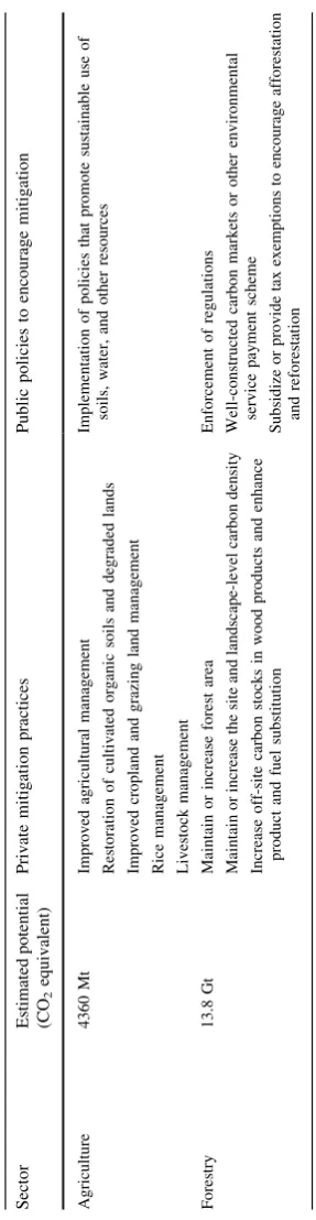
In order to reduce the concentration of greenhouse gases in the atmosphere, governments can provide incentives to consumers and firms to reduce the amount of gases that are released, finance research programs to develop technologies to further reduce emissions, or increase the earth’s absorption capacity (for example, by expanding the forest area). Policies can be market-based (i.e., through the price system) or impose the use of certain practices and/or technologies on firms. Since the latter is usually more expensive and less flexible than the former, economists recommend that policies focus on creating market signals that discourage emissions. Market-based policies can regulate either the price of emissions (through taxation) or the amount of emissions allowed, leaving the determination of the price of carbon to the market by letting firms trade ‘‘emissions rights’’. Under perfect and symmetric information both approaches should render the same results, but the presence of uncertainties and information asymmetries about the dangers of greenhouse gas emissions and the cost of controls implies that they will have different consequences. The decision as to which type of regulation to use depends mostly on which uncertainty entails the greatest dangers. A perception that the consequences of increasing emissions could be catastrophic should favor cap and trade schemes, while the risk of emissions regulation entailing large costs should induce policymakers to adopt tax schemes.
Table2 presents a series of public policies and private measures that have the potential to either reduce the amount of greenhouse gases that are released into the atmosphere or increase the absorption capacity of the planet.
3.2 Adaptation policies and practices
Sect.5 of this paper) which are the best policies to be implemented. Table3 presents a list of public and private adaptation measures divided by sector. However, policies can be also classified by scope (distinguishing between local and regional or short- and long-term policies), timing (proactive or reactive), or the agent that carries them out (either private or public).
3.3 Development policies
In addition to traditional adaptation policies, an increase in the quantity and quality of public goods such as health, education, and access to clean water might also help reduce the adverse effects of climate change, while being useful even if its consequences do not materialize. That is why some studies call them ‘‘no-regret’’ policies. Although the overlap between adaptation and development is large (OECD 2009), and what constitutes a no-regret policy for some countries may be considered pure adaptation for others, there are some well-known policies that could increase the resilience of society to climate change even if that is not their primary goal. These policies address drivers of vulnerability, regardless of whether they have an origin in climate change. Moreover, development generally is accompanied by economic growth, which reduces the share of GDP used for adaptation, making more policies feasible. Among these policies, probably the most salient are the extension of access to public services such as education and health.
Education has proven to have many spillovers related to productivity increases and diversification, allowing societies to reduce their dependence on weather-sensitive activities. Education can be tailored to address issues that would arise as the climate changes, such as protection against heat waves and infectious diseases. Improvement in public education can be achieved by investing in infrastructure such as more and better-equipped schools, reducing class size, decentralizing decision-making, and improving the monitoring of teachers (Duflo2001; Galiani and Pe´rez Truglia2013).
Poor public health is a major barrier to economic growth in developing economies, and is exacerbated by the proliferation of slums, which is a side effect of economic growth when combined with the uncontrolled increase in urban populations. According to UN-Habitat (2003), almost 1 billion people currently live in such environments. Slum dwellers suffer from poor infrastructure and poor provision of such public services as piped water and drainage and waste disposal systems, and they are reluctant to invest in homes for which property rights are not well established. In 2008, nearly 40 % of the world population lacked adequate sanitation facilities, and more than 10 % used inadequate sources of water (Duflo et al.2012). This has adverse health consequences such as diarrheal diseases, which account for 21 % of child mortality in developing countries.
Table 3 Examples of adaptation practices and policies by sector
Sector Private adaptation practices Public adaptation policies Water
resources
Usage of low-flow toilets and showers
Re-use of cooking water Leak repair
Rainwater collection Installation of canal linings Use of closed conduits Water recycling
Expansion of drip irrigation Increase of water harvesting
Change the location or height of water intakes Use of artificial recharge
Raise dam heights Increase canal size Sediment removal
Construction of reservoirs and hydroplants Implementation of well fields and inter-basin water
transfers
Coastal zones
Migration and retreat Afforestation
Dike, sea-wall, and embankment building Implementation of beach and shore nourishment Construction of shelters and enhancement of
building standards Modification of land use
Establishment of early warning systems Agriculture Adoption of pest-, drought-, and
heat-resistant crops Change of planting dates Crop mixing
Improvements in irrigation efficiency
Use of water harvesting Implementation of terracing and
deep ploughing R&D on resistant crops
Improvements in pest management through biological controls
Diffusion of resistant crops among farmers Construction of dams and irrigation systems Provision of institutional support to diffuse
information on climate change and adaptation possibilities
Enhancement of agricultural trade Promotion of efficient use of resources Livestock Change in grazing and breeding
management
Change in mix of grazers or browsers
Change in location of watering points
Change in supplemental feeding Use of windbreaks to protect soil
from erosion
Use of vegetative barriers or snow fences to increase soil moisture
Development of large-scale watershed projects and breeding programs
Discouragement of use of marginal land and protection of degraded areas
Implementation of veterinary animal health services
Energy Increased implementation of cooling equipment
Improved efficiency of cooling systems
Improvement of thermal insulation in buildings
Enhanced energy efficiency and thermal shell standards
barriers in terms of their effectiveness, including high provision costs, low willingness to pay due to lack of complete knowledge of the benefits of these services, and liquidity constraints that constrain connection to existing networks. Institutional constraints—such as lack of coordination between different levels of government or collective action problems—can also be behind the service deficit. These issues must be taken into account and overcome in order to ensure that policies that improve access to sanitation services are effectively implemented (Duflo et al.2012).
With regard to the provision of water in general, in regions where water is already scarce (such as the Andean region of South America and northern Mexico), implementation of irrigation systems can increase the land available for agriculture and livestock, and thus increase food security. Increasing the availability of safe water is also fundamental in cities, mostly for people living in slums. Policies in this direction include improvements in distribution systems and investment in trans-basin infrastructure, as well as the development of water markets (Grafton et al. 2011) and implementation of water management practices. In countries where water availability is unevenly distributed during the year (World Bank 2010), increased water harvesting and expansion of storage capacity would significantly alleviate the problem.
Latin America is subject to extreme events mostly related to the ‘‘El Nin˜o’’ southern oscillation. This phenomenon involves the increase of the Pacific Ocean’s surface temperature along the coasts of Ecuador and Peru. Scientists have found that this anomaly can affect atmospheric circulation features and produce persistent temperature and precipitation anomalies in many regions, such as wetter conditions along the west coast of tropical South America and subtropical latitudes of North and South America. The opposite is evidenced during ‘‘La Nin˜a’’ episodes. According to Magrin et al. (2007), these anomalies negatively affect such sectors as agriculture and livestock, human health (through the outbreak of disease vectors that develop in warm and humid environment), and both public and private infrastruc-ture (since floods that are consequence of increased rainfall can damage houses, roads, power networks, etc.). They note that these consequences have become more frequent in the last three decades, in line with what has happened as a result of other highly unusual extreme weather events.
Table 3 continued
Sector Private adaptation practices Public adaptation policies Biodiversity Increase of protected areas
Establishment of ecological corridors for migration of species
Active management of wild populations outside of protected areas
Maintenance of captive populations Ecological restoration
The Tropical Ocean-Global Atmosphere Program has been in place since the 1980s to reduce some of the aforementioned effects by predicting El Nin˜o trends and related phenomena. Magrin et al. (2007) note that the program can predict most of these phenomena with lead times between 3 months and a year.
Other development strategies include the improvement of communication and transport infrastructure. In most developing countries, roads are often not paved and thus become impassable whenever there is an extreme climatic event. Thus, paving and maintaining roads (in some cases using building standards that make them withstand more extreme temperatures and enhanced risk of flooding), together with implementing transportation safety measures, will enhance the competitiveness of the economy and promote growth.
Finally, the provision of property rights where they are not well defined or are subject to expropriation can promote investment and enhance economic growth (Galiani and Shargrodsky2010). Economic growth in turn raises per capita income and protects households from transitory negative shocks, while investment in homes (among other things) helps protect them from climate change.
As can be seen, the range of alternatives for governments to cope with climate change is vast. However, developing countries often face tight budget constraints that may force them to choose only a subset of such policies. The next section presents a theoretical framework to address this issue.
4 Coping with climate change: theoretical framework
The first model that quantified the economic impact of climate change was developed by Nordhaus (1994). The Dynamic Integrated Model of the Climate and the Economy (DICE) is a growth model that takes into account emissions, greenhouse gas concentrations, climate change, and the possibility of implementing mitigation policies. An increase of mitigation expenditures alleviates future temperature increases, which in turn reduces damage to the economy. Nordhaus shows that a harmonized carbon tax across all countries and sectors, with a value that increases over time, is, within the setup of his model, the most efficient policy to reduce emissions. The DICE model was updated in 2008 to include the latest data obtained from more recent research. It assumes that all countries agree on implementing the carbon tax in order to reduce emissions, but, as explained previously, international agreements to date have instead focused primarily on cap and trade schemes rather than on Pigouvian taxes, and compliance among countries has been rather low. Under these circumstances, mitigation costs are substantially higher than those predicted by the DICE model.
impact if they are focused on mitigation policies. The question then is: what is the relevant mix of policies for developing countries?
de Bruin et al. (2009) include adaptation as a decision variable in both the DICE model and another model entitled RICE (Regional Integrated Model of the Climate and the Economy). They conclude that an effective adaptation policy is particularly important when suboptimal mitigation policies are implemented. A drawback of this model is that adaptation is not viewed as an investment, but rather as a ‘‘reactive’’ expenditure that accrues its benefits only during the period when the adaptation measures are in place.
Chisari et al. (2013) also draw on the original DICE model, but include both adaptation and mitigation expenditures as decision variables. The paper calibrates the different relevant parameters of the model to match those of the United States, Brazil, and Chile, representing large, medium, and small economies, respectively. In this model, adaptation reduces the negative effect of pollution on GDP. The authors find that the ratio of expenditures on adaptation to mitigation will be larger the smaller the country, and what they call ‘‘environmentally small’’ economies will concentrate only on adaptation policies, since in these countries only adaptation presents positive net benefits to society. They also show that small economies that are unable to spend enough on adaptation may end up spending less on mitigation owing to their impoverishment as a result of negative climate shocks.
We extend the work in Chisari and Galiani (2010) and Chisari et al. (2013) and present a simple two-period model in which a government must decide how much to spend to cope with climate change, taking as given what other countries do. We incorporate uncertainty about the effects of climate change by introducing two possible states of the world in the second period: one in which there are no changes in climate, and another in which the climate changes and their impact depend on how well the country is adapted to them. Although we draw on the Chisari et al. (2013) framework, our model is not concerned with economic growth for simplicity. Yet we arrive at some of their results: namely, that an environmentally small country should refrain from spending on mitigation practices in the absence of a large international agreement to do so. As stated in the previous section, in the presence of cumulative uncertainties around climate change, low-income countries may be better off investing in traditional development policies that will also reduce their vulnerability to climate change. Because of this, we include public investment as an additional policy variable that has a positive future effect irrespective of climate change, although it provides a higher utility to the representative agent in the presence of global warming.
4.1 A model of government spending under the potential of climate change
Consider first a representative agent that maximizes its utility over two periods:
U¼u c0;ð gÞ þð1pð ÞE Þu c
H 1;g
þpð ÞE u cL 1;cg
1þr :
produced by a concave technologyFin the stock of capital. In the second period, the climate changes with probability p. This probability depends on the level of emissions in the atmosphereE. When the climate worsens, a share 1ð bÞof output is lost. This share is a strictly concave function on the amount the government has invested in adaptation (denoted bya) in the previous period.4Also, under a ‘‘bad’’ scenario (one in which consumption is lowcL
1), the agent derives more utility from
public investment than if temperature had not risen. Consider, for example, the expansion of piped water networks: if it becomes more difficult to access drinking water, then the previous investment made by the government becomes more valuable for the private sector). This means thatc[1.
Thus, the constraints faced by the representative agent are:
F i0ð Þ gð1dÞma¼c0þi F i0ð þiÞ ¼cH1
bð Þa F i0ð þiÞ ¼cL1:
4.1.1 The representative agent’s problem
In the first period, the agent chooses how much to consume and how much to invest in order to increase the next period’s consumption. We can thus state the problem of the representative agent as:
max
i U¼u F i0ð ð Þ igma;gÞ þ
1pð ÞE
ð Þu cH 1;g
þpð ÞE u cL 1;cg
1þr : ð1Þ
The first-order condition for this problem is then:
oU
oi ¼
oFð Þ:
oi
ou
ocð1þp bð ð Þ a 1ÞÞ
|fflfflfflfflfflfflfflfflfflfflfflfflfflfflfflfflfflfflfflfflfflffl{zfflfflfflfflfflfflfflfflfflfflfflfflfflfflfflfflfflfflfflfflfflffl} Marginal benefit
ou
ocð1þrÞ
|fflfflfflfflfflffl{zfflfflfflfflfflffl} Marginal Cost
¼0: ð2Þ
This is nothing but the standard Euler equation for intertemporal decisions, which states that the optimal level of private investment is the one that equates the benefits (the first term of the equation) to its costs (the second term) at the margin. Here, both the costs and benefits are expressed in terms of consumption (the cost is present consumption to which the private agent has to give up, and the benefit is the future consumption the agent will enjoy thanks to a higher product level). Although we cannot obtain an explicit equation for the optimal level of private investment, we know from the implicit function theorem thati¼iðg;a;m;p;rÞ.
4.1.2 The government’s problem
The government seeks to maximize the representative agent’s utility by optimally choosing in the first period how much to invest in public goods and adaptation and mitigation expenses using the lump-sum taxes it levies on the private sector. In doing this, the government takes into account how the agent will react to a change in any of these decision variables. We shall make the (realistic) assumption that spending on adaptation is always positive in the extreme case in whichp¼1.
Given the large uncertainty surrounding climate change and its impact on the economy, a government may also want to wait until more information or better technology becomes available in order to allocate its resources more wisely. However, waiting for uncertainty to ‘‘resolve’’ might not be a good strategy (at least for the time being) if, as mentioned earlier, the variance of the effects of climate change tends to increase rather than decrease as scientists uncover more ‘‘unknown unknowns’’ that may influence or be influenced by global warming. Other reasons to act early are the possibility of obtaining short-term benefits, locking in long-lasting benefits (Agrawala and Fankhauser 2008), and the presence of irreversibilities, which means that sometimes it could be too late to act. Thus, the problem the government faces is:
max
g;m;aU¼u F i0ð Þ i
g 1
d
ð Þma; g
ð Þ
þð1pð ÞE Þu F i0;i ð Þ;g
ð Þ þpð ÞE uðbð Þa F i0;ð iÞ;cgÞ
1þr ;
ð3Þ
subject toE¼eþað Þm F ið Þ;m0;a0;g0.
The first constraint here shows that the level of emissions that affects the economy is partly due to the emissions of the rest of the world (which are taken as given) and those of the country itself. The latter depends on past output, as the literature suggests (it takes time for pollution to have an impact in the form of climate change), and how much has been invested in mitigating those emissions. For this,a2 ð0;1Þandoa
om[0.
Note that since mitigation is a global public good, it is possible that developing countries receive transfers from developed countries in the context of a global agreement to reduce greenhouse gas emissions (such as the Clean Development Mechanism) in order to encourage them to make efforts in this respect. Thus,d is the share of mitigation expenditure that the government receives from the rest of the world. This parameter has no upper bound: compensation could very well exceed developing countries’ expenses.
The first-order conditions for this problem are:
oU
om¼
ou
oc 1d
þ oi
om
1þr
ð Þ þou
oc
oF
oi
oi
omþpð ÞE
ou
oc
oF
oi
oi
omðbð Þ a 1Þ
þop
oE
oE
om u
Lð Þ : uHð Þ:
oU
og ¼
ou
oc 1þ
oi
og
1þr
ð Þ þð1pð ÞE Þ ou
oc
oF
oi
oi
ogþ
ou
og
þpð ÞE ou
oc
oF
oi
oi
ogbðaÞ þc
ou
og
0 ð5Þ
oU
oa ¼
ou
oc 1þ
oi
oa
1þr
ð Þ þð1pð ÞE Þ ou
oc oF oi oi oa
þpð ÞE ou
oc
ob
oaF ið Þ þbðaÞ
oF
oi
oi
oa
0 ð6Þ
m0;a0;g0 ð7Þ
moU
om¼0;g
oU
og ¼0;a
oU
oa ¼0: ð8Þ
Although it will not be possible to provide an explicit form for any of the endogenous variables, we can derive some results from these equations:
Result 1a:Mitigation expenditure for environmentally small economies is highly dependent on foreign transfers.
First, we see from Eq. (8) that ifm6¼0, then Eq. (4) must hold with equality. Rearranging the terms, we show that the benefits of the last dollar spent on mitigation must equal its marginal cost:
op
oE
oE
om u
Lð Þ : uHð Þ:
¼ou
oc 1d
þ oi
om
1þr
ð Þ
þou
oc
oF
oi
oi
om½pð ÞE ð1bð Þa Þ 1:
The direct benefits of mitigation expenditure are related to whether it can significantly reduce the stock of emissions. As in Chisari et al. (2013), we expect this effect to be marginal in environmentally small economies, relative to the emissions generated by large economies. In our model, this is analogous to saying thatoomEffi0. If this is so, then the left side of the equation would tend to zero.
On the other hand, the costs of a dollar spent on mitigation net of transfers from the rest of the world are in terms of the resources that will not be available for the representative agent for consumption. Transfers from the rest of the world could reduce this cost or even turn it into a net benefit. The sign of oi
omis still uncertain.
Public spending on mitigation could crowd out private investment, or conversely encourage it. Whichever the effect of mitigation on private investment, the sign of the right-hand side of the equation will ultimately be determined by the share of mitigation expenditure that is financed by the rest of the world. In fact, mitigation efforts in developing countries to date have been closely tied to transfers from developed countries, as we shall see later.
This result follows from the previous one. Assume d¼0: Then the Euler equation that determines the level of mitigation expenditure becomes:
op
oE
oE
om u
Lð Þ : uHð Þ:
¼ou
oc 1þ
oi
om
1þr
ð Þ þou
oc
oF
oi
oi
om½pð ÞE ð1bð Þa Þ 1:
Since for environmentally small economiesoE
omffi0, and because the sign of the
right-hand side of the equation is indeterminate, it follows that the equality will probably not hold. This means that the optimal level of mitigation for these ‘‘environmentally small’’ economies will be zero.
Result 2: Investment in public goods that are useful even in the absence of climate change will be positive irrespective of the size of the economy.
Let us take a look at Eq. (5). If government spending is positive, then its optimal level is the one that accomplishes:
ou
og½1þpð ÞðE c1Þ ¼
ou
oc 1þ
oi
og
1þr
ð Þ ½1pð ÞE ð1bðaÞÞou
oc
oF
oi
oi
og:
ð9Þ The marginal cost of government investment in public goods (left-hand side) is measured in terms of the consumption and investment from which the individual cannot benefit today and in the future, net of the future forgone output due to global warming. However, as this investment enters directly into the representative agent’s utility function, its benefits are enjoyed in both states of nature, and in fact they are enhanced if climate change takes place. This means that there is always a nonzero level of optimal public spending.
Result 3:Public spending on adaptation will be positive in environmentally small economies only above an idiosyncratic risk of climate change.
Inspecting Eq. (6) and rearranging the terms in such a way that the marginal benefit of adaptation is on one side of the equality and its marginal cost is on the other:
pð ÞE ou
oc
ob
oaF ið Þ ¼
ou
oc 1þ
oi
oa
1þr
ð Þ ð1pð ÞE Þ ou
oc oF oi oi oa
pð ÞE ou
ocbðaÞ
oF
oi
oi
oa: ð10Þ
Marginal costs (left-hand side) are in terms of both present consumption and investment that becomes unavailable as adaptation increases (although we still do not know how investment will respond to adaptation), and how this affects future consumption, both if climate change does not occur (in which case adaptation expenditure proves wasteful) or if it does occur. The marginal benefit of the last dollar spent on adaptation (right-hand side) is expressed in terms of the share of production that would be lost if that dollar were spent elsewhere.
of a dollar spent on adaptation increases, and its cost decreases. Taking this and our assumption thata6¼0 whenp¼1 together with the continuity of the functionbin its argumentaleads to the conclusion that there is a threshold levelpover which it is worthwhile to assign funds for adaptation investments. Of course, this threshold will depend on each country’s characteristics, such as its level of investment or how vulnerable it is to climate change.
4.1.3 Comparative statics
Now that we have stated the first-order conditions for the four variables of interest (remember that as we set the individual’s problem, consumption will result as a ‘‘residual’’ after the individual has chosen how much to invest for the next period), we can derive the four implicit functions for the optimal level of expenditure on each of them:
i ¼i gð ðp;c;rÞ;aðp;rÞ;p;rÞ
g ¼gðp;c;rÞ
a ¼aðp;rÞ
m ¼0:
We would like to know how an exogenous change in the probability of climate change affects the optimal allocation of public spending between pure adaptation and no-regret investments, leaving the tax level unchanged (this means that dgþda¼0). Note that this is possible only for environmentally small economies, which for the most part take this probability as given. For simplicity we shall first assume that private investment does not react to changes in public investment, so oi
og¼o i
oa¼0:Then, the FOC of the government’s problem result in:
oU
og ¼ u
0
cð1þrÞ þð1pð ÞE Þu
0
g F i
ð Þ;g
ð Þ þpð ÞE cu0gðbF ið Þ ;gÞ ¼0
oU
oa ¼ u
0
cð1þrÞ þpb
0u0
cF i
ð Þ ¼0:
We differentiate these equations with respect to p and apply Cramer’s rule to solve foroogpandoa
op. Normally, we would expectu
00
c;g to be non-negative, and if the
representative agent’s utility is separable in consumption and public investment, then it will be zero. In what follows, we will assume this property holds.
Result 4: The share of adaptation expenditure in the government’s budget is nondecreasing inp.
scenario increases, the marginal benefit of adaptation increases with respect to that of traditional public investment. The fact that adaptation is positive whenppalso means that the marginal benefit of an extra dollar spent on adaptation is greater than that spent on public goods. This should be reinforced as p approaches 1, which means that abovepthe equilibrium level of adaptation increases to the detriment of traditional public goods as global warming’s threat becomes more plausible.
From our results it is evident that in the actual situation where there is not a binding international agreement on mitigation that includes developing countries, the choice of the these countries is restricted to policies that can either enhance resilience against climate change or traditional development policies in any scenario. Only in the context of a global agreement in which all nations commit to reduce greenhouse gas emissions and emerging countries are given proper incentives to participate should developing countries make efforts to reduce the concentration of greenhouse gases in the atmosphere. The choice among the policies to be implemented is nevertheless not a trivial one. In fact, it will depend on which policies yield greater benefits for a given budget. A framework for analyzing this is provided in the next section.
5 Cost–benefit analysis as a framework to choose policies
From the model presented in the previous section, we can only infer the types of strategies worth considering under different contexts. However, we can say nothing about which policies should be adopted. Under no financial constraints, a government should implement every policy that yields a net benefit to the population. However, this case is highly uncommon, particularly in developing countries. Thus, the task of policymakers is to choose among a wide range of options. Why is it preferable to enhance building standards for homes instead of giving land titles to slum dwellers? Is it better to connect more homes to the water network or to enhance water storage capacity in order to overcome droughts? Questions like these can only be answered by using a metric to rank different policies. The most widely used one is to compare the benefits of each policy to its cost, which is known as cost–benefit analysis. This section presents a brief description of the approach and how it is implemented.5
Cost–benefit analysis begins with the determination of the relevant population, followed by an evaluation of policy effectiveness. Ideally, impact assessment takes the form of a controlled experiment or a quasi-experiment in which statistically similar groups are contrasted.
In many cases, the whole range of benefits associated with interventions cannot be fully estimated, but it is possible to infer those effects using economic models. This is particularly relevant when the policies in question have equilibrium effects. Even in those cases, it is still desirable to combine modeling with experimental or quasi-experimental variability in a way to that permits model validation.
5
When policy effects are empirically assessed, they are expressed in physical units. When dealing with policies that have the same outcome variable, this should be enough for comparison. However, when comparing policies in different sectors it is necessary to use a common unit of measure, which is usually money. To determine the value that should be assigned to a certain change in physical units, researchers use the concepts of ‘‘willingness to pay’’ and ‘‘willingness to accept’’ compensation for a change in an individual’s utility. If a policy benefits an individual, willingness to pay tells how much the individual would give up for the policy to be implemented. This amount should equal the sum that would render the individual as well as if the policy were not applied at all. Conversely, willingness to accept is the amount that the individual would be compensated if the policy were not implemented, which should be equal to what gives the individual as much utility as the individual would have, all else being equal, with the new policy. While in theory the two measures should be similar, in practice willingness to accept compensation has been found to be considerably larger in magnitude than willingness to pay compensation.
If effects are constrained to private goods and services, then their prices should reflect an individual’s willingness to pay and a producer’s willingness to accept compensation for those goods and services. However, in many cases (notably in environmental policy), some of these costs and benefits are not privately but rather socially borne or enjoyed. The problem with externalities is that their value cannot be directly observed, because they are not individually traded in the market. In this case, measures of willingness to pay or willingness to accept must be obtained indirectly. For nonmarket goods that have ‘‘use value’’ (meaning that their value is related to actual, planned, or possible use of the good, such as a recreational park), revealed preference techniques and stated preference techniques may be used. In contrast, if value has to be given to ‘‘nonuse goods’’ (those to which individuals attach value even if they are not subject to any possible use, as could be the mere existence of a species), then only the latter approach is viable.
Revealed preference techniques are used to value nonmarket effects by observing individuals’ behavior (in particular, purchases) in real markets, with the premise that this behavior reveals something about the implicit price of a related nonmarket good. Approaches vary according to the characteristics of the good that is subject to valuation, including hedonic pricing (Davis2004; Roy 2008), travel cost (Kremer et al.2011), and averting behavior, among others. Each approach has its strengths and weaknesses, and recent empirical findings warn about the validity of some of the assumptions behind them (Madajewicz et al.2007; Jalan and Somanathan2008; Devoto et al.2012; Tarozzi et al.2011).
When a good or service is valued only for its mere existence, then revealed preference approaches are not suitable for obtaining agents’ willingness to pay for it. Instead, researchers turn to stated preference techniques. These involve creating a hypothetical market for the good or service in question, and asking a random sample of individuals to reveal their maximum willingness to pay for a change in its provision.
differentiated by its attributes and levels, one of which should be its price. Individuals are asked to rank the alternatives or choose their preferred one. The baseline scenario must be included as a way of allowing respondents to choose a ‘‘no-policy’’ option.
5.1 Aggregation and decision rules
Once average willingness to pay for costs and benefits has been obtained, it has to be aggregated across the relevant population of those who benefit and those who lose. With this, it is then possible to determine whether the policy should be adopted on efficiency grounds. The first rule that may come up is to approve any policy that achieves a Pareto improvement, i.e., that makes some people better off while leaving nobody worse off. However, policies with this characteristic are exceptional. A less restrictive condition for a policy to pass a cost–benefit analysis is that the value of aggregate benefits outweighs that of aggregate costs. If this is the case, those who benefit can compensate the losers and still be better off. This is called a potential Pareto improvement. A general formula for determining if a project is acceptable under this criterion would be:
X
i;t
wiWTPGið1þsÞ t
X
i;t
wiWTPLið1þsÞ t
0:
If costs and/or benefits accrue at different moments (as is typically the case with adaptation investments), then they should all be expressed at present value. Hence
1þs
ð Þt is the discount factor.
In turn,wiis the weight given to individuali’s willingness to pay. Policymakers
may have equity as well as efficiency concerns, which are the base of cost–benefit analysis. For example, wi¼0 means that an individual is excluded from the
analysis. If guided only by efficiency, a project might be carried out even if gains are mostly enjoyed by the rich and losses fall disproportionately on the poor, as long as the former outweigh the latter. However, distributional issues are at the core of climate change policies. For this, two main approaches have been suggested: explicit or implicit weighting. In the former, weights are imputed based on results from previous studies. Implicit weighting, on the other hand, entails determining the required weights for a policy to pass a cost–benefit analysis and then asking if those weights are reasonable either in relation to empirical studies or political or ethical considerations.
5.2 Uncertainty and the value of information
passes the cost–benefit analysis, then it is said that the measure is ‘‘robust’’ with respect to the different assumptions made. In contrast, if the decision about the policy depends on the assumptions made, then other considerations should guide the final decision, including the reasonableness of the assumptions.
In this context, it is possible that delaying implementation of a policy that entails some irreversibility will allow for more information to be gathered and better estimates to be made. In fact, every policy’s cost–benefit analysis can and should be compared to that of the same policy implemented at a different moment in order to determine the optimal timing of implementation. If as a result of the acquisition of information the net benefits of delaying the implementation of a policy are effectively larger than those of implementing it now, then the value of that information equals the difference in net benefits between the two timings. Then the policy is said to have a ‘‘quasi-option value’’, analogous to a financial option, which allows for buying or selling an asset at a certain moment after additional information has been obtained. However, waiting may entail costs as well as benefits. If an adaptation policy is postponed, it is possible that an extreme event will occur while the environment or societies are still vulnerable. Thus, the costs of waiting have to be accounted for alongside the value of information that could be obtained.
In conclusion, cost–benefit analysis focuses the direction of a generic research agenda. Every policy under consideration should be thoroughly studied before being implemented: their effects must be rigorously assessed and their benefits weighted against their costs. Only in this way can a program be compared to others that also claim to increase welfare or reduce the harm provoked by a threat such as climate change. Cost–benefit analysis is extensively used in developing countries, but studies of this kind for adaptation (particularly in Latin America) are still lacking. Without them, it will be difficult to determine the right path to follow in the years ahead.
It must be noted that the range of available policies is too wide to conduct a cost– benefit analysis of each of them. Instead, researchers should start with those areas where climate change could be most harmful. For example, the agriculture and livestock sectors, which are among the most important sectors in Latin America, are at the mercy of weather conditions if they do not have the proper infrastructure and technology in place. The next section is thus devoted to exploring a particular aspect that might be relevant for adaptation in these sectors because of their importance for Latin America. The section will also look at how cost–benefit analysis could be implemented in this particular case.
6 Increasing adaptive capacity: technology adoption and learning
in the agricultural sector
avoid decreases in crop yields (Parry et al.2004; Gay et al.2004; Pinto et al.2002), and water scarcity may require the use of more efficient irrigation techniques, such as drip irrigation.
Agriculture is crucial for Latin America’s economy because it represents almost a quarter of its exports (World Bank 2012). Yet its productivity has grown at a slower rate than in developed countries for the past 50 years (IDB 2015). This signals that the sector is not using the best available technology, and a side effect of this is that it is more vulnerable to the consequences of climate change than it could be. In the past, researchers have identified different causes for this lag in technology adoption, including irrational behavior, scale economies, risk aversion, credit constraints, and lack of knowledge about the best way to adopt a technology.
Although producers are always considered rational and profit-maximizing agents, it is possible that this assumption does not always hold true. An example of this is when producers discount the future with a hyperbolic factor, which leads to a present bias. Duflo et al. (2011) find evidence of this for the use of fertilizer in Kenya. Producers often delay the purchase of fertilizer until it is too late to use it. The researchers found that using subsidies to encourage producers to buy fertilizer at the time of harvest (when they are relatively more liquid) increases uptake by more than 50 %, which in turn raises the producers’ income.
Another possibility is that some kind of market failure is preventing a portion of producers from adopting new technologies. For example, incomplete insurance may lead only wealthier producers to adopt newer, riskier inputs. Credit constraints may have the same consequence: only producers who are able to pay the cost of the new technology up front are able to adopt it, thus restraining adoption of the technology to those with more wealth. Lack of infrastructure and market power may also alter the profits that farmers obtain, thus reducing the incentives for investment. As has been properly documented in urban areas, land market failures in the form of poor property rights also affects incentives to invest in technology improvement. Although there is not much evidence on the presence of these types of inefficiencies in the agricultural sector, some studies have been able to so identify them, at least indirectly.6
Finally, it is possible that producers are not aware of the existence of more profitable technologies, or do not entirely know how to use them to obtain the greatest benefit. Typically, the adoption of technology involves some kind of learning, including evaluating if a new technology is more profitable than the existing one, and adapting it to the environment in which it will be implemented. For example, Duflo et al. (2008) randomly selected a group of farms in Western Kenya and divided them into small plots. For 3 years, each plot was planted with maize (either using traditional varieties or hybrid seeds) using different amounts of fertilizer, including that recommended by the country’s Ministry of Agriculture. Even though the authors found that yields increased the most when using the recommended package, mean and median profits were highly negative, and the