R E G U L A R A R T I C L E
Open Access
Improving official statistics in emerging
markets using machine learning and mobile
phone data
Eaman Jahani
1*, Pål Sundsøy
2, Johannes Bjelland
2, Linus Bengtsson
3,4, Alex ‘Sandy’ Pentland
1,5and
Yves-Alexandre de Montjoye
5,6,7*Correspondence: [email protected] 1Institute for Data, Systems and Society, Massachusetts Institute of Technology, 50 Ames Street, E18-407A, Cambridge, MA 02142, USA
Full list of author information is available at the end of the article
Abstract
Mobile phones are one of the fastest growing technologies in the developing world with global penetration rates reaching 90%. Mobile phone data, also called CDR, are generated everytime phones are used and recorded by carriers at scale. CDR have generated groundbreaking insights in public health, official statistics, and logistics. However, the fact that most phones in developing countries are prepaid means that the data lacks key information about the user, including gender and other
demographic variables. This precludes numerous uses of this data in social science and development economic research. It furthermore severely prevents the
development of humanitarian applications such as the use of mobile phone data to target aid towards the most vulnerable groups during crisis. We developed a framework to extract more than 1400 features from standard mobile phone data and used them to predict useful individual characteristics and group estimates. We here present a systematic cross-country study of the applicability of machine learning for dataset augmentation at low cost. We validate our framework by showing how it can be used to reliably predict gender and other information for more than half a million people in two countries. We show how standard machine learning algorithms trained on only 10,000 users are sufficient to predict individual’s gender with an accuracy ranging from 74.3 to 88.4% in a developed country and from 74.5 to 79.7% in a developing country using only metadata. This is significantly higher than previous approaches and, once calibrated, gives highly accurate estimates of gender balance in groups. Performance suffers only marginally if we reduce the training size to 5,000, but significantly decreases in a smaller training set. We finally show that our indicators capture a large range of behavioral traits using factor analysis and that the framework can be used to predict other indicators of vulnerability such as age or socio-economic status. Mobile phone data has a great potential for good and our framework allows this data to be augmented with vulnerability and other information at a fraction of the cost.
Keywords: mobile phone metadata; machine learning; data-driven development;
vulnerable populations
1 Introduction
Mobile phone metadata, automatically generated by our phones and recorded at large-scale by carriers, have the potential to fundamentally transform the way we fight diseases, collect official statistics, or design transportation systems. Scientists have compared the recent availability of these large-scale datasets to the invention of the microscope [] and new fields such as Computational Social Science [] are emerging. Mobile phone data have, for instance, already been used to study human mobility and behavior in cities [], the geographical partitioning of countries [], and the spread of information in social net-works []. The potential of large-scale mobile phone data is particularly great in devel-oping countries. Indeed, while reliable basic statistics are often missing or suffering from severe bias [] mobile phones are one of the fastest growing technology in the developing world with penetration rates ranging from % in Uganda to % in Ghana []. In de-veloping countries, mobile phone data has, for instance, already been used to model the spreading of malaria [] and dengue fever [], and to perform real-time population density mapping []. Orange made large samples of mobile phone data from Côte d’Ivoire and Sénégal available to selected researchers through their Data for Development Challenges []. Last year, the United Nations called for the use of mobile phone data in support of the Sustainable Development Goals [].
Pseudonymous mobile phone metadata datasets contain fine-grained information on who called whom for how long and from where. These are available in real-time and often with historical data over several years. However, in developing countries, the vast ma-jority of subscriptions are prepaid []. This means that SIM cards can be easily bought anywhere and that the carrier, and therefore the researchers using the data, often lack even the most basic information on users such as gender, age and employment status. This lack of socio-demographic information in mobile phone data sets is a major impediment to the use of mobile phone data for development. Predicting socio-demographic characteristics of users in anonymous mobile phone data sets can, e.g., enable more efficient delivery of information to specific groups such as maternal health information. Determining socio-demographic composition of a group can enable needs-based distribution of relief services to displaced populations during crises, and provide socio-demographically disaggregated census [], mobility [], and migration data. We here report on a framework to extract insightful behavioral indicators from standard mobile phone metadata and how these in-dicators can be used to augment a dataset with key demographic variables, including vul-nerability information, at a small surveying cost. In this paper, we explore how different socio-demographic variables of a user can be reliably predicted from mobile phone data and how this information could be used at-scale by NGOs like Flowminder, reducing the data collection cost by approximately two orders of magnitude.
], cyclones in Bangladesh [, ] and more fine-grained poverty estimates [, ]. This translates into more efficient allocation of relief resources by operational agencies, as well as a better understanding of the distribution of the need for specialized services such as maternal and newborn health care during crises. While operator data has been shown to predict infectious disease spread, e.g. for cholera [], it is likely that these models can be considerably improved by accounting for differential socio-economic composition of travelers.
Using data from over .M people in two countries, one in Europe (EU) one in South Asia (SA),awe first show how a small training sample of k people per country is enough to predict a user’s gender with high accuracy. We then show how this can be used in two real-world scenarios: finding women in a dataset - e.g. to send them prenatal care mes-sages - and correctly predicting the gender balance (men-women percentages) - e.g. in a given geographical region for census purposes. Second, we investigate the potential of our framework to predict individual characteristics beyond gender. We analyze the behavioral indicators produced by our framework and argue that they are useful in prediction tasks beyond gender. We then evaluate their applicability in other prediction tasks to further assess the vulnerability of a person: age and household income. All our predictions are made solely based on behavioral features extracted from standard mobile phone data. We anticipate that including location information as an extra feature to the models, even at a coarse level (urban or rural), will further improve our prediction performance. The rest of the paper is structured as follows: In Section , we review related work. In Section , we describe our framework and behavioral indicators as well as the two datasets we use. In Section , we describe our results on gender and evaluate our approach in two real-world use cases. In Section , we investigate the potential of our framework to predict individual characteristics beyond gender. In Section , we compare our prediction performance with related work and we conclude in Section .
2 Related work
Previous work showed how a user’s gender could be predicted from their digital bread-crumbs (e.g. browsing history) [], first name [, ], and writing style [, ]. More precisely, Murray et al. used latent semantic analysis and neural networks [] and Hu et al. used a Bayesian framework and a bipartite pages-users network [] to predict a user’s gender from their browsing history. In a highly publicized work, Kosinski et al. used lin-ear regression to predict a user’s gender from their Facebook likes []. Burger et al. used standard machine learning on Twitter data (profile and tweets data) [] while Rao et al. used stacked-SVM (support vector machine) algorithm on tweets []. Ciot et al. extended previous work on Twitter data to non-English contexts []. Deitrick et al. predicted gen-der information from e-mail conversation using neural networks [] and Peersman et al. using SVMs on chat data []. Finally, Seneviratne et al. used the list of installed Apps to predict gender [] while Malmi and Weber showed how the same information can be used for prediction of other demographic variables such as age, race, marital status and income [].
(RF) to predict regional crime [] and poverty [] and, at individual-level, to predict loan repayments []. Blumenstock found that while men and women exhibit statistically sig-nificant differences in how they use their phones in Rwanda, these differences are mainly determined by economic factors, and therefore lead to marginal prediction performance []. Mehrotra et al. defined a fixed effect regression model and estimated the differences in communication patterns of men and women inter-day, intra-day, on holidays and on specific politically important days [].
Dong et al. report interesting results in predicting user’s gender and age in a mobile phone social graph using a double-dependent Factor Graph model []. While such a homophily-based method is very efficient at predicting a small portion of missing labels in the full social graph, they are inefficient for our use case focused on low and middle income countries where the vast majority of the labels are missing and collecting training data through surveys is costly.
The most relevant works to ours are reported in [–]. Martinez et al. used SVM and RF as well as a custom algorithm based on k-means on features derived from stan-dard mobile phone data to predict gender information []. Similarly, Herrera-Yagüe and Zufiria applied multiple machine learning algorithms on features incorporating node-level activity, ego-network strucuture and homophily to predict age and gender []. Sar-raute et al. used SVM and logistic regression on features to predict gender and age information []. They also discussed a label-propagation algorithm that achieved high accuracy in age-prediction by exploiting the homophily in the network. We outperform [–] in a practical context (see Section ) and none of these discuss the minimum level of training data required to obtain the best achievable performance using only the node-level attributes. The homophily-based algorithms, while outperforming the other models, are designed for and can be trained only on a significant fraction of the dataset. A more detailed comparison is provided in Section .
3 The framework and data
3.1 Bandicoot behavioral indicators
We developed an open-source python toolbox, bandicoot [], to compute more than behavioral indicators from individual-level standard mobile phone metadata. These behavioral indicators, which we use as features, range from simple ones such as number of calls, number of texts, and average call duration to more advanced ones such as the text response rate, radius of gyration, and entropy of visited places. The indicators are first gen-erated on a weekly basis, and then both their means and standard deviations are computed over the three month period. Some indicators admit a single number on a weekly basis, e.g. the number of texts or the number of active days in a week. Others are defined as an empir-ical distribution over a week period, e.g. call duration and the interevent time. For these, we compute both the weekly mean but also maximum, minimum, median, standard devi-ation, and skewness. Finally, we also computed all the indicators on a weekly basis while separating weekdays from weekends and day times from night times. Indicators are coded as: name_weeklysplit_dailysplit_intertype_wsumstat_asumstat with
Table 1 All 31 indicator families computed by Bandicoot divided by the temporal unit of the distribution they measure
Temporal period Indicator families
Over weeks active_days__callandtext number_of_contacts__text number_of_contacts__call percent_nocturnal__text percent_nocturnal__call
percent_initiated_conversations__callandtext percent_initiated_interactions__call response_rate_text__callandtext entropy_of_contacts__text entropy_of_contacts__call percent_pareto_interactions__text percent_pareto_interactions__call number_of_interactions__text number_of_interactions__call number_of_interaction_in__text number_of_interaction_in__call number_of_interaction_out__text number_of_interaction_out__call number_of_antenna
entropy_of_antennas percent_at_home radius_of_gyration frequent_antennas
Within weeks call_duration__call
response_delay_text__callandtext balance_of_contacts__text balance_of_contacts__call interactions_per_contact__text interactions_per_contact__call interevent_time__text interevent_time__call
Indicators over weeks take a single value per week and measure themeanandstdover several weeks. Indicators within weeks admit multiple values within each week which are aggregated bymin, max, mean, std, skewness, kurtosis. The weekly aggregated values are then aggregated over consecutive weeks usingmeanandstd.
weeklysplitcan beallweek,weekday, orweekend.dailysplitcan be all-day,day, ornight.intertypedefines the type of interactions over which the indica-tor is computed,call,text, orcallandtext.wsumstatis only there for indicators which admit a distribution per week such ascall_durationorinterevent_time.
wsumstatindicates the summary statistics used on the within-week distribution:min,
maxbut alsomean,median,std,skewness, andkurtosis. Finally,asumstat indi-cates the summary statistics used across weeks, eithermean- which captures the general activity level - orstdfor the over-weeks regularity. While the indicators coming from the same function will often be correlated, they might capture different behavioral traits. In total, we examined indicators derived from functions (see Table ). More in-formation on the Bandicoot toolbox, the behavioral indicators, and the various filters and summary statistics can be found online at http://bandicoot.mit.edu. Note that all the indi-cators are computed at individual-level thereby avoiding issues of incomplete graphs, e.g. given a specific carrier’s market share.
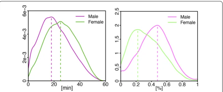
Figure 1 Most discriminative feature in EU (left): the maximum text response delay during the week; in SA (right): percent of calls initiated by the person during the weekend nights.The dashed lines indicate the modes of the distributions, with 25 minutes for females and 18 minutes for males in EU and 22% for females and 48% for males in SA.
using SVM-Lasso with an L-norm penalty (forward selection) []. The indicator is de-fined between and min. As shown in Figure , women take more time than men to re-spond to text messages during the week. The average response delay for men is minutes (std = .) and for women min (std = .). In the south Asian country, the most dis-criminative feature is the percent of calls initiated by the person during the weekend nights (percent_initiated_interactions__weekend__night__call__mean). Here, men initiated a lot more call on weekend nights (μ= ., std = .) than women (μ= ., std = .) [Figure ].
3.2 Proposed methodology
We consider Bandicoot’s main usage to be prediction of population characteristics at an individual level. For such use cases, we propose the following methodology:
. Collect raw CDRs for a random selection ofncustomers.ndetermines the total
train and test size and is usually restricted by cost of collecting labels through phone surveys. While more training data usually leads to better performance, we here show that, above a certain level, obtaining more training data does not improve the performance significantly, thus putting an upper limit on the total cost of phone surveys. It is important for the CDRs to be collected over a long enough period (at least a month) to capture regularity in calling patterns. Furthermore, CDRs for train, test and prediction data must be collected during the same time period, so that the same conditions, for example price rates, apply equally to all customers. Note that due to these variations, it is important for the model to be retrained frequently. A cost effective way to start is by using new CDRs but for the same set of customers for whom labels were obtained before.
. Extract Bandicoot’s indicators for the random set of users whose CDRs and labels
prediction. In this paper, we do not include any such external information and make our predictions solely based on behavior patterns present in CDRs.
. Bandicoot extracts more than features from raw CDRs. If the training data is
limited, it is important to limit the feature space to only the set of indicators that are relevant to the prediction problem. Elastic net, Lasso SVM, Tree based algorithms and Univariate statistical tests are some examples of possible feature selection algorithms. In this study, we used Lasso SVM as part of our cross-validation pipeline.
. The variable of interest might exhibit a non-linear behavior against several Bandicoot indicators. For example, income and average duration of call might co-vary in a non-linear fashion across urban and rural areas. Therefore, it is recommended to examine prediction performance with algorithms that can capture such non-linearities (e.g. KNN or Random Forest) and compare them with linear algorithms such as SVM and Logistic Regression.
If the objective is to estimate an aggregate population parameter (e.g. average age), we can obtain individual predictions using the same methodology above (while being very careful to have the same TPR and FPR on our training and validation sets) and then ag-gregate the predictions to the population level.
3.3 Datasets
This study was performed using two anonymized mobile phone datasets containing months of standard metadata in a developed country (European country,n= k, % male) and in a developing country (South Asian country,n= k, % male). The Bandi-coot behavioral indicators [] were computed from the raw mobile phone data and made available to us by an unnamed carrier. Label information was available for all users through contract information in the European country (EU) and were collected through phone sur-veys in the south Asian country (SA). All of our reported results are based on the subset of users who had at least active days per week on average throughout the months period (.% of SA and .% of EU full data).
4 Gender prediction
We trained all our algorithms using -fold cross validation and tested them on a separate, previously unseen, samples of k people in EU and k people in SA. We trained five dif-ferent algorithms: logistic regression (Logistic), SVM with linear kernel (SVM-Linear) and radial basis function kernel (SVM-RBF), k-nearest neighbors (KNN), and random forests (RF). As our original feature space consisted of a large number of features, we used a cross validated SVM with L-penalty for feature selection prior to training any of the five mod-els. This feature selection was particularly important when we artificially reduced the size of the training set to k people or less. Therefore, throughout the paper, the training phase always refers to an initial feature-selection, followed by a cross-validation to find the best parameters.
our framework. Balancing is particularly important for our second use case of estimating gender balance. To further balance our model to make it equally good at identifying men and women, we tried either modifying the penalty term for each gender (inversely pro-portional to its relative frequency in the training set) or creating a balanced train set by undersampling the majority class while retaining the original population distribution in the test set. Results were equivalent and we kept the latter: undersampling the majority class. All results were obtained using Bandicoot v.. and scikit-learn v..
4.1 Overall performance
Phone usage and how it distinguishes men and women or high- and low-income people is likely to be affected by the geographical and cultural context of the country and to vary with time. Indeed, changes in pricing schemes, penetration rates, and the socio-economic development of the country means that training sets have to be country and time specific. This differs strongly from traditional classification problems. For instance, training sets used for image classification are less time - and potentially culturally-sensitive. This is an important part of our application as labeled data will need to be specifically acquired through surveys to train the model with a collection cost largely linear with the number of labels. The applicability of our work is thus largely dependent on the performance of the framework with a small training set: to be useful, our framework needs to reach a high accuracy with a training set that is a small fraction of the considered dataset.
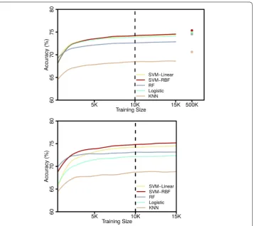
Figure shows the performance of our framework as a function of the size of the training set and that our framework reaches a high accuracy with a small training set. Indeed, with a training set of k people, we already reach an accuracy of .% in both EU and SA, and AUC of . in EU and . in SA. Increasing the size of the training set beyond k people only marginally increases accuracy. In EU, we reach an accuracy of .% with k people and, in SA, an accuracy of .% with k people. SVM-RBF gives, in both EU and SA, the best accuracy with training sets≥ people and KNN the worst. On the entire dataset, RF and SVM-Linear give, in EU, an accuracy similar to SVM-RBF while logistic and KNN give a lower accuracy. In SA, SVM-Linear, Logistic, and RF have similar performances but lower than SVM-RBF. KNN has a lower accuracy. As mentioned before, all these results are obtained on subset of users who are active at least days per week on average during the months CDR period. Figure shows how the performance results change as we vary this data preprocessing threshold.
Figure 2 Accuracy in EU (top) and SA (bottom) as a function of the size of the training sample. We reach an accuracy beyond 74% with training sets of 10k people. In case of data scarcity, we can further reduce the training size to 5k with minimal deterioration in performance. SVM-RBF reaches a higher accuracy than other algorithms in both cases for training sets larger than 5k people. In EU, increasing the training set size from 15k to 500k only increases the best accuracy by 1%.
Figure 3 Accuracy and AUC in EU (left) and SA (right) as a function of the minimum required level of activity.The model is trained and tested on a subset of users who are on average active x days per week, throughout the 3-months CDR period. As we increase this minimum required threshold, x, the coverage decreases and the performance slightly improves.
areas when compared to the EU country. KNN is the only algorithm that can effectively circumvent such data complexity but performs poorly on the bottom % of the users.
Figure 4 Accuracy in EU (left), SA (right) on the top x% of the users the algorithms are the most confident about. In EU accuracy scales linearly with the top x% of the dataset while in SA most algorithms plateau around the top 60% of the database.
Table 2 Performance measures for SVM-RBF at different confidence thresholds in EU and SA (Positive=Women,Negative=Men): True Positive Rate (TPR), False Negative Rate (FNR), True Negative Rate (TNR), False Positive Rate (FPR)
Country Confidence subset TPR FNR TNR FPR
EU 25% 90.0 10.0 89.1 10.9
100% 74.5 25.5 74.4 25.6
SA 25% 83.9 16.1 77.0 23.0
100% 67.2 32.8 76.4 23.6
of the dataset. In our application, misclassifying women (or men) at a higher rate than the other - which might arise in unbalanced datasets - would be highly problematic. These results validate the effectiveness of our balancing scheme in SA and the applicability of our results.
The performance results above are obtained by training the model on K samples. However, if training data was particularly hard or expensive to acquire in a new coun-try or if slightly lower accuracy is enough for the application at hand, out of of the algorithms we tried reach good level of accuracy with smaller training set. For instance, Figure shows that SVM-RBF has an accuracy of .% in EU and .% in SA with a training set of only people. This means that in scenarios where coverage need not be % or roughly % accuracy is sufficient, large-scale mobile phone datasets can be labeled with gender information at a fraction of the cost of traditional national surveys (roughly two order of magnitude) as we only need to survey a couple thousand individu-als for labeling a database containing millions.
4.2 Use cases
We here showed that large-scale mobile phone datasets can be labeled with gender infor-mation at a fraction of the cost. In this section, we will now evaluate the applicability of our framework for two use-cases. All the results are using a training set of k people with SVM-RBF unless specified otherwise.
.. Finding women in a dataset
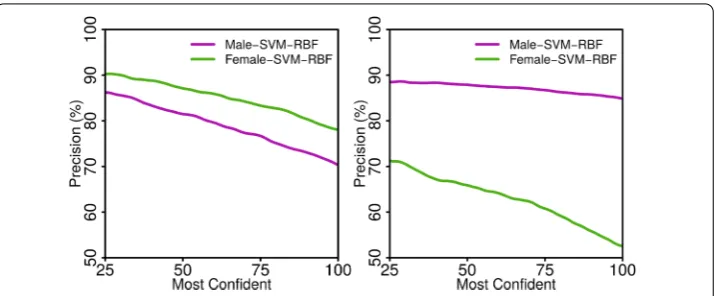
Figure 5 Precision for finding women (and men) in EU (left) and SA (right) as a function of the percentage of women that are in the dataset and which we are trying to find.The precisions are highly influenced by how balanced the datasets are. Our method reaches much higher precision than random (54% in EU and 29% in SA).
to [] is the first use case we evaluate the effectiveness of our framework against. More specifically, we focus on the task of finding a given set of users that are the most likely to be women in a dataset, e.g. to send them prenatal care educational and child immuniza-tion messages [] or informaimmuniza-tion about the importance of measles immunizaimmuniza-tion []. More precisely, we here evaluate the effectiveness of our framework at identifying a cer-tain number of women out of the dataset.
Figure shows the precision of our framework at finding women (and men) in EU and SA. Precision is, if we pick the % of people in the dataset that we think are the most likely to be women, the percentage of them who are actually women. Precision in find-ing women in the EU ranges from .% when we try to find % of the women in the dataset to .% when trying to find all of them. Precision for men is respectively .% and .%. We obtain similar results with other algorithms. Precision is slightly higher for women, probably as the dataset is slightly unbalanced towards women (% men). In SA, precision ranges from .% to .% for women and from .% to .% for men. The precision for women is to % lower than for men. This is likely due to the fact that the dataset (and therefore test set) is highly unbalanced towards men (% men) thus making it much harder to find women even with our balancing of the training set. Nevertheless, our method reaches a precision up to . times higher than random.
.. Estimating gender balance
Figure 6 True versus predicted gender balance in EU (left) and SA (right).
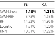
Table 3 Mean average error in predicting gender balance
EU SA
SVM-Linear 1.10% 1.21% SVM-RBF 3.75% 1.53%
RF 14.53% 11.95%
Logistic 1.51% 1.20%
KNN 18.51% 17.22%
individual in the group as a man or woman. While this gives us a first estimation of the gender balance of this group, we know from our training set that we have non-zero true and false positive rate [Table ]. This means that, in a group in SA composed only of men, we would still - on average - predict that we have women. We therefore control for the false positive and negative rates as:
calibrated= predicted
TPR–FPR– FPR
TPR–FPR ()
Figure shows that our predicted gender balance with SVMs and Logistic Regression is very close, both in the EU and SA to the true gender balance of the group. Table shows that the mean absolute error of our predicted gender balance using SVM-Linear is .% in EU (r= .) and .% in SA (r= .). This means that we are, on average, at most one or two percent off from the true men-women percentage in the group. The predicted ratio after calibration is not as impressive in the case of random forest and KNN, mainly due to the difference in train and test recalls. Both achieved a considerably higher recall in the train set compared to test set, and as a result their calibration was not aggressive enough. For example, the EU recall of RF in train set is . larger than test set while both train and test recalls are around . in the case of SVM-Linear.
5 Generalization
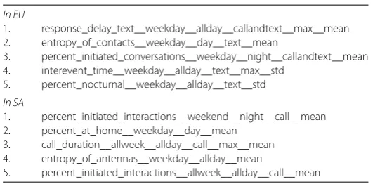
Table 4 Most predictive features in EU and SA according to the Linear SVM with L1 penalty
In EU
1. response_delay_text__weekday__allday__callandtext__max__mean 2. entropy_of_contacts__weekday__day__text__mean
3. percent_initiated_conversations__weekday__night__callandtext__mean 4. interevent_time__weekday__allday__text__max__std
5. percent_nocturnal__weekday__allday__text__std
In SA
1. percent_initiated_interactions__weekend__night__call__mean 2. percent_at_home__weekday__day__mean
3. call_duration__allweek__allday__call__max__mean 4. entropy_of_antennas__weekday__allday__mean
5. percent_initiated_interactions__allweek__allday__call__mean
5.1 Factor analysis
We extract more than behavioral indicators from standard mobile phone data. Re-sults from the previous section shows that, when used as features, these behavioral in-dicators contain information useful to predicting individual’s gender. We here use factor analysis and results from features selection to argue that our framework is applicable to general prediction tasks, at group or individual level, using mobile phone data.
We first use exploratory factor analysis to investigate the correlation structure in our indicators and group them into unique behavioral traits, called factors. This allow us to describe the variety of underlying behaviors our indicators capture []. In the analysis, we standardized all of our indicators to unit variance and mean zero to give all of them equal weight. We then use Horn’s parallel test, where the scree of factors in the data is compared with that of a random data matrix of the same size, to determine the number of latent fac-tors present in the data. Comparing the eigenvalues from the data with the corresponding ones in the random data allow us to separate the true factors (higher eigenvalue) from the spurious ones. We then use the least square criteria to extract the factors and perform an oblique rotation to simplify their interpretation, allowing different factors to be slightly correlated. We consider a feature to belong to a factor if its factor loading is above ..
The parallel test suggest that our behavioral indicators computed in SA contain la-tent factors and in EU. This emphasizes the fact that even if our indicators are derived from core functions (see Table ), they capture a broad set of latent behavioral traits. This points to the applicability of our framework beyond gender information. Visual anal-ysis of the extracted factor structure (not shown) suggest that daily and nightly indicators from the same family often belong to different factors. The same is true for weekday versus weekend stressing the importance of separating indicators by time of the day or day of the week.
Figure 7 Accuracy as a function of the number of features in EU (left), SA (right).
Table 5 The most (top 3) and least (bottom 3) predictive factors of gender in the South Asian data
Top indicators in the factor Proportion of variance Weighted F1 score
call_duration__weekday__day__call__min__std 0.4% 0.68 call_duration__weekday__day__call__median__std
call_duration__weekday__day__call__min__mean
call_duration__weekend__night__call__min__mean 0.5% 0.68 call_duration__weekend__night__call__min__std
call_duration__weekend__night__call__median__std
percent_initiated_interactions__weekday__day__call__mean 0.3% 0.66 percent_initiated_interactions__allweek__day__call__mean
percent_initiated_interactions__weekend__day__call__mean
number_of_interaction_in__allweek__allday__text__std 0.6% 0.37 number_of_interaction_in__allweek__day__text__std
number_of_interaction_in__weekday__allday__text__std
number_of_interaction_in__weekday__allday__text__mean 0.8% 0.37 number_of_interaction_in__allweek__allday__text__mean
interactions_per_contact__weekday__allday__text__max__mean
balance_of_contacts__weekend__night__text__max__mean 0.5% 0.53 balance_of_contacts__weekend__night__text__median__mean
balance_of_contacts__weekend__night__text__min__mean
For each factor, the three indicators with the highest loading are shown here. The F1 score is weighted by the class frequency to account for the data imbalance. Despite not being predictive of gender, the bottom three factors capture a significant amount of variance in the data.
Figure 8 Income prediction confusion matrix with colors encoding the number of data points in each income bin.The numbers within each cell represent the absolute size normalized by the total size of the true income bin. Note that since income categories are sorted from very poor (1) to very rich (5), the deviation of our income predictions from truth is small for most income bins.
and outgoing calls and rate adjustment throughout the day, the balance of contacts is also a potential candidate for income prediction. While the question of what other variables these factors could predict and what can and cannot, in general, be predicted with high accuracy from mobile phone data remains, the evidence here suggest that our framework and behavioral indicators capture behavioral traits that exhibits good levels of variation in the population and are likely to be suitable candidates for other prediction tasks.
5.2 Age and socio-economic prediction
To further demonstrate the applicability of our framework to general prediction tasks, we report on two promising results on predicting age and income from mobile phone data. The ability to predict income, in particular, has important development implications and can be used to inform policy decisions regarding welfare resource allocation, inequality or economic growth [].
Figure 9 Age prediction in the EU data using elastic-net achievesR2= 0.35, when data points are
weighted according to their inverse frequency. An elastic net model with uniform weights achieves a higherR2= 0.47 (not shown). Actual ages are grouped into 10 year bins.
of information on user home location. As noted in [, ], income is often correlated with geo-location and varies greatly from rural to urban areas. Its correlation with behav-ioral indicators might also vary drastically between urban areas. Therefore, we expect the performance of our income prediction to improve significantly if we were to add coarse location dummy variables in the feature space. Inclusion of such dummy variables in our model will also enable us to capture any non-linearity that might arise among different rural and urban areas.
Second, we use our framework to predict age in the EU data. We here use a training set of , people and a test set of , people. Since the exact ages as opposed to age groups were available, we used a cross-validated elastic net linear regression model with sample weights set to the reciprocal of age frequency. Our model achieves aR= . on the test set with mean absolute error of . years. Note that if the model is trained with uniform weights, our features can achieve a higherR= . and mean absolute error of . years, but at the expense of imbalance in predictions with higher error for less frequent ages. Figure shows the box plot of our age predictions against the actual age combined in year bins, when sample weights are assigned to take into account the frequency im-balance of age values. For the purpose of comparison with related works, we also treat age prediction as a multi-classification problem with balanced age classes. A logistic regres-sion model with One-vs-Rest scheme achieves an accuracy of .% on the full data, an improvement of . times over a random baseline of %, and % when we reduce the coverage to % of the most confident predictions.
The results from these two other applications further emphasize the generality of our framework for various predictions tasks using mobile phone metadata.
6 Comparison with previous work
instead of average route distance between consecutive calls, we use radius of gyration as defined in [] as a measure of mobility. Furthermore, we do not include any information on expense patterns which, if included, will increase our prediction performance for gen-der, but more importantly for socio-economic status and age as observed in []. Similar to our findings, Martinez et al. reported statistically significant differences among males and females in the distribution of all features with the exception of average route distance. In contrast, we find that mobility indicators such as radius of gyration and percent at home, are among the most discriminating features between males and females, especially in SA. Their SVM and RF models on the full data achieved an accuracy of % in predicting gender. The authors achieved higher accuracy by sacrificing coverage and restricting the prediction to individuals who belong to predominantly male-only or female-only k-means clusters and reported an accuracy of % with % coverage and % with % coverage. In comparison, we obtain an accuracy of % when the coverages are % (SA) and % (EU), and an accuracy of at least % when coverage is % (both SA and EU). It should be noted that our most powerful features achieve an accuracy of .% in SA and .% in EU with % coverage (see Figure ). We attribute these improvements to our a richer set of discriminating indicators and effective feature selection among our large feature-set for any particular prediction task.
Herrera-Yagüe and Zufiria [] designed features that are most relevant to prediction of gender and age (as a multi-classification problem with classes). The features captured two types of information: communication patterns across isolated links ( features) and ego-networks structures ( features). They evaluated the prediction performance of each feature category using multiple learning algorithms and reported an accuracy of % for gender prediction and % for age prediction using only isolated link features. Features based on ego-network structure achieved slightly lower accuracies. The authors greatly improved the isolated link predictions (to % for gender and % for age) by including the gender and age of the neighboring node as an extra feature in the model. Access to alters’ age provided a much larger performance boost, since it is widely known that age-homophily is much stronger than gender-age-homophily in social networks. The final model used aggregated predictions from isolated links, ego-network features and alters gender or age in a single model and achieved an accuracy of % for gender and % for age prediction. Our models include all the isolated link information discussed in [], but aggregated into single features for each node. Furthermore, we don’t employ any informa-tion on the network structure since we would like the predicinforma-tion to be possible for each nodesolely based on their own communication behavior and without having access to the full communication behavior of their neighbors,as in most cases (for practical or market share reasons), we do not have access to such information. More importantly, we achieve a minimum gender prediction accuracy of % compared to their %, without harness-ing the inherent homophily in the network, since features designed based on homophily would require obtaining the true label of a large portion of the full communication net-work, a costly process as mentioned for []. Nevertheless, we expect our performance to greatly improve, in particular for age prediction, by incorporating the information on the neighboring nodes in the model.
Table 6 Comparison of our framework with the most related work [44–46]
Martinez Herrera-Yagüe Herrera-Yagüe (Homophily)
Sarraute Sarraute (Homophily)
EU SA
Gender 0.56 0.55 0.65 0.663 – 0.743 0.745
(100%) (100%) (100%) (100%) (100%) (100%)
0.80 – – 0.814 – 0.80 0.80
(3%) (12.5%) (76%) (65%)
Age – 0.24 0.51 0.37 0.434 0.568 –
(100%) (100%) (100%) (100%) (100%)
– – – 0.527 0.623 0.819 –
(12.5%) (12.5%) (12.5%)
The number outside (inside) the parentheses indicates the accuracy (the data coverage of such accuracy). Columns with homophily show the results when the labels of adjacent nodes, in addition to individual node-level attributes, were used as another feature in the algorithm. Martinez did not discuss age-prediction and Herrera-Yagüe did not report accuracy at different coverage level. Furthermore, Herrera-Yagüe predicted age into 6 categories, thus it should be compared against a random 0.16 baseline. Sarraute and our model predicted age into 4 categories, thus they should be compared against a 0.25 random baseline. The best models reported in [45, 46] leverage the homophily structure in the network, while our models do not exploit any information based on the homophily; as such a more justified comparison would be based on only the node-level attributes.
prediction, the features when used with lasso SVM achieved an accuracy of .% on the full data and .% with .% coverage, which we outperform with a % accuracy on the full data and % accuracy with at least % coverage. The authors treated the age-prediction as a multi-classification problem with categories and reported an accuracy of % on the full data and % with .% coverage. Similar to [], the authors observed a strong age homophily and a weak gender homophily, therefore they used a separate label-diffusion algorithm which predicted the age of a node only by exploiting the homophily structure in the network. The diffusion algorithm significantly improved upon the multi-nomial regression, which solely relies on node attributes, and achieved an accuracy of .% on the full data and .% with .% coverage. However as mentioned before, the label diffusion method suffers from the unavailability of true labels in real-world tasks for large portion of the network. Through an exploratory analysis, the authors discovered that % of the variation in their dataset could be explained by principal components mainly related to activity levels and communication direction. In comparison, in our framework (EU) and (SA) components explain % of the variation while components only account for % of variations in both EU and SA. This points to the richness of our feature space and its ability to achieve higher prediction performance. It should be noted that in our feature space, the top components are related to call interevent times (accounting for % of variance) in SA and number of active week nights (accounting for % of variance) in EU.
Table summarizes the comparison above. Note that for the purpose of comparison with [], we implemented age-prediction as a multi-classification problem using logistic regression.
7 Conclusion
We validate the applicability of our framework in two real-world use cases (finding women and estimating gender balance) and show how our method performs well in both cases. We find women with a precision of up to . times better than random in SA and we are able to estimate the gender balance of a group with an MAE of a couple of percent. We finally showed our framework to be applicable to other prediction tasks, by demonstrating that our behavioral indicators () capture a large range of behavioral factors and () can be used to predict other demographic variables, such as age with regressionR= . and income with % improvement in the multi-classification accuracy over random guessing. Mobile phone data have a great potential for good and our work shows how these high-resolution data can be augmented with gender, age, income and other information. In developing countries, a national survey is usually conducted only every few years as such large-scale surveys cover millions of households and are extremely costly. Our proposed framework can provide an alternative source of timely information to traditional census methods at a fraction of the cost, since only a few thousand survey responses is enough to achieve a comparable accuracy at individual and aggregate levels. Our work opens-up the way to large-scale and low-cost labeling of mobile phone datasets and their use in research, economic policy making and humanitarian applications.
List of abbreviations
CDR, SVM, KNN, RF, SA, EU, RBF, TPR, FPR
Availability of data and materials
For contractual reasons, we are unable to publicly provide the data used in this study. Bandicoot is an opensource software under MIT license and can be found at http://bandicoot.mit.edu/. The code used for obtaining the results is available online at https://github.edu/eamanj/demographics_prediction.
Competing interests
The authors declare that they have no competing interests.
Funding
This material is based upon work supported by the National Science Foundation Graduate Research Fellowship under Grant No. 1122374. Any opinion, findings, and conclusions or recommendations expressed in this material are those of the authors(s) and do not necessarily reflect the views of the National Science Foundation. Yves-Alexandre de Montjoye was partially supported by a grant from the Media Lab and Wallonie-Bruxelles International.
Authors’ contributions
Eaman Jahani, Pål Sundsøy, Johannes Bjelland, Linus Bengtsson, Alex ’Sandy’ Pentland and Yves-Alexandre de Montjoye designed the research. Pål Sundsøy and Johannes Bjelland generated the data. Eaman Jahani performed the analysis and obtained the results. Eaman Jahani, Pål Sundsøy, Linus Bengtsson and Yves-Alexandre de Montjoye wrote the paper.
Author details
1Institute for Data, Systems and Society, Massachusetts Institute of Technology, 50 Ames Street, E18-407A, Cambridge, MA 02142, USA.2Telenor Research, Snarøyveien 30, Oslo, 1331, Norway.3Flowminder, Roslagsgatan, Stockholm, Sweden. 4Department of Public Health Sciences, Karolinska Institute, SE-171 77, Stockholm, Sweden.5Media Lab, Massachusetts Institute of Technology, 20 Ames Street, E14, Cambridge, MA 02142, USA.6Department of Computing, Imperial College London, 180 Queens Gate, London, SW7 2RH, UK. 7Data Science Institute, William Penney Laboratory, Imperial College London, London, SW7 2RH, UK.
Acknowledgements
The authors thank Luc Rocher and William Navarre for their help with the Bandicoot toolbox, Asif Iqbal for help with the data, Prof. Joachim Meyer from Tel-Aviv University for his great ideas regarding factor analysis and Jake Kendall for useful discussions.
Endnote
a For contractual reasons, we cannot name the specific countries.
Publisher’s Note
Springer Nature remains neutral with regard to jurisdictional claims in published maps and institutional affiliations.
References
1. Giles J (2012) Making the links. Nature 488(7412): 448-450
2. Lazer D, Pentland AS, Adamic L, Aral S, Barabasi AL, Brewer D, Christakis N, Contractor N, Fowler J, Gutmann M et al. (2009) Life in the network: the coming age of computational social science. Science 323(5915): 721
3. Toole JL, de Montjoye Y-A, González MC, Pentland AS (2015) Modeling and understanding intrinsic characteristics of human mobility. In: Gonçalves B, Perra N (eds) Social phenomena. Springer, Cham, pp 15-35.
4. Ratti C, Sobolevsky S, Calabrese F, Andris C, Reades J, Martino M, Claxton R, Strogatz SH (2010) Redrawing the map of Great Britain from a network of human interactions. PLoS ONE 5(12): 14248
5. Miritello G, Moro E, Lara R (2011) Dynamical strength of social ties in information spreading. Phys Rev E 83(4): 045102 6. Stuart E, Samman E, Avis W, Berliner T (2015) The data revolution. finding the missing millions. London: ODI. Available
at http://www.developmentprogress.org/sites/developmentprogress.org/files/case-study-report/data_revolution_-_finding_the_missing_millions_-_final_20_april.pdf
7. Cell Phones in Africa: Communication Lifeline.
http://www.pewglobal.org/2015/04/15/cell-phones-in-africa-communication-lifeline/. Accessed: 2015-10-17 8. Wesolowski A, Eagle N, Tatem AJ, Smith DL, Noor AM, Snow RW, Buckee CO (2012) Quantifying the impact of human
mobility on malaria. Science 338(6104): 267-270
9. Wesolowski A, Qureshi T, Boni MF, Sundsøy PR, Johansson MA, Rasheed SB, Engø-Monsen K, Buckee CO (2015) Impact of human mobility on the emergence of dengue epidemics in Pakistan. Proc Natl Acad Sci 112(38): 11887-11892 10. Deville P, Linard C, Martin S, Gilbert M, Stevens FR, Gaughan AE, Blondel VD, Tatem AJ (2014) Dynamic population
mapping using mobile phone data. Proc Natl Acad Sci 111(45): 15888-15893
11. de Montjoye Y-A, Smoreda Z, Trinquart R, Ziemlicki C, Blondel VD (2014) D4d-senegal: the second mobile phone data for development challenge. arXiv:1407.4885
12. Independent Expert Advisory Group on a Data Revolution for Sustainable Development (2014) A world that counts: mobilizing the data revolution for sustainable development
13. ITU: ITU releases latest global technology development figures. Accessed: 2015-10-17
14. Wilson R, zu Erbach-Schoenberg E, Albert M, Power D, Tudge S, Gonzalez M, Guthrie S, Chamberlain H, Brooks C, Hughes C, Pitonakova L, Buckee C, Lu X, Wetter E, Tatem A, Bengtsson L (2016) Rapid and near real time assessments of population displacement using mobile phone data following disasters : the 2015 Nepal earthquake. PLoS Curr 1, 1-26
15. Lu X, Bengtsson L, Holme P (2012) Predictability of population displacement after the 2010 Haiti earthquake. Proc Natl Acad Sci 109(29): 11576-11581
16. Lu X, Sundsøy P, Wetter E, Qureshi T, Canright G, Monsen K, Bengtsson L, Wrathall D, Nadiruzzaman M, Iqbal A, Tatem A (2016) Detecting climate adaptation with mobile network data in bangladesh: anomalies in communication, mobility and consumption patterns during cyclone mahasen. Climatic Change
17. Lu X, Wrathall D, Sundsøy P, Wetter E, Qureshi T, Canright G, Monsen K, Bengtsson L, Wrathall D, Nadiruzzaman M, Iqbal A, Tatem A (2016) Unveiling hidden migration and mobility patterns in climate stressed regions: A longitudinal study of six million anonymous mobile phone users in bangladesh. Global Environmental Change
18. Steele J, et al. (2016) Predicting poverty using mobile phone data and satellite data. In submission 19. Sundsøy P (2016) Can mobile phone usage predict illiteracy? arXiv:1607.01337 [cs.AI]
20. Bengtsson L, Gaudart J, Lu X, Moore S, Wetter E, Sallah K, Rebaudet S, Piarroux R (2015) Using mobile phone data to predict the spatial spread of cholera. Sci Rep 5, 8923
21. Hu J, Zeng H-J, Li H, Niu C, Chen Z (2007) Demographic prediction based on user’s browsing behavior. In: Proceedings of the 16th international conference on world wide web, WWW’07. ACM, New York, pp 151-160. 22. Mislove A, Lehmann S, Ahn Y-Y, Onnela J-P, Rosenquist JN (2011) Understanding the demographics of Twitter users.
ICWSM 11, 5
23. Liu W, Ruths D (2013) What’s in a name? Using first names as features for gender inference in Twitter. In: AAAI spring symposium: analyzing microtext
24. Otterbacher J (2010) Inferring gender of movie reviewers: exploiting writing style, content and metadata. In: Proceedings of the 19th ACM international conference on information and knowledge management, CIKM’10. ACM, New York, pp 369-378.
25. Argamon S, Koppel M, Fine J, Shimoni AR (2003) Gender, genre, and writing style in formal written texts. Text: Interdisciplin J Study Discourse 23, 321-346
26. Murray D, Durrell K (2000) Inferring demographic attributes of anonymous Internet users. In: Masand B, Spiliopoulou M (eds) Web usage analysis and user profiling. Springer, Berlin, pp 7-20.
27. Hu J, Zeng H-J, Li H, Niu C, Chen Z (2007) Demographic prediction based on user’s browsing behavior. In: Proceedings of the 16th international conference on world wide web. ACM, New York, pp 151-160.
28. Kosinski M, Stillwell D, Graepel T (2013) Private traits and attributes are predictable from digital records of human behavior. Proc Natl Acad Sci 110(15): 5802-5805
29. Burger JD, Henderson J, Kim G, Zarrella G (2011) Discriminating gender on Twitter. In: Proceedings of the conference on empirical methods in natural language processing. Association for Computational Linguistics, pp 1301-1309. 30. Rao D, Yarowsky D, Shreevats A, Gupta M (2010) Classifying latent user attributes in Twitter. In: Proceedings of the 2nd
international workshop on search and mining user-generated contents. ACM, New York, pp 37-44. 31. Ciot M, Sonderegger M, Ruths D (2013) Gender inference of Twitter users in non-English contexts. In: EMNLP,
pp 1136-1145
32. Deitrick W, Miller Z, Valyou B, Dickinson B, Munson T, Hu W (2012) Author gender prediction in an email stream using neural networks
33. Peersman C, Daelemans W, Van Vaerenbergh L (2011) Predicting age and gender in online social networks. In: Proceedings of the 3rd international workshop on search and mining user-generated contents. ACM, New York, pp 37-44.
34. Seneviratne S, Seneviratne A, Mohapatra P, Mahanti A (2015) Your installed apps reveal your gender and more! SIGMOBILE Mob. Comput. Commun. Rev. 18(3): 55-61 doi:10.1145/2721896.2721908
36. de Montjoye Y-A, Quoidbach J, Robic F, Pentland AS (2013) Predicting personality using novel mobile phone-based metrics. In: Proceedings of the 6th international conference on social computing, behavioral-cultural modeling and prediction, SBP’13. Springer, Berlin, pp 48-55.
37. Chittaranjan G, Blom J, Gatica-Perez D (2011) Who’s who with big-five: analyzing and classifying personality traits with smartphones. In: 2011 15th annual international symposium on wearable computers (ISWC). IEEE, New York, pp 29-36.
38. Bogomolov A, Lepri B, Staiano J, Oliver N, Pianesi F, Pentland A (2014) Once upon a crime: towards crime prediction from demographics and mobile data. In: Proceedings of the 16th international conference on multimodal interaction. ACM, New York, pp 427-434.
39. Blumenstock J, Cadamuro G, On R (2015) Predicting poverty and wealth from mobile phone metadata. Science 350(6264): 1073-1076
40. Bjorkegren D, Grissen D (2015) Behavior revealed in mobile phone usage predicts loan repayment. Available at SSRN 2611775
41. Blumenstock J, Gillick D, Eagle N (2010) Who’s calling? Demographics of mobile phone use in Rwanda 42. Mehrotra A, Nguyen A, Blumenstock J, Mohan V (2012) Differences in phone use between men and women:
quantitative evidence from Rwanda. In: Proceedings of the fifth international conference on information and communication technologies and development. ICTD’12. ACM, New York, pp 297-306.
43. Dong Y, Yang Y, Tang J, Yang Y, Chawla NV (2014) Inferring user demographics and social strategies in mobile social networks. In: Proceedings of the 20th ACM SIGKDD international conference on knowledge discovery and data mining. ACM, New York, pp 15-24.
44. Frias-Martinez V, Frias-Martinez E, Oliver N (2010) A gender-centric analysis of calling behavior in a developing economy using call detail records. In: AAAI spring symposium: artificial intelligence for development 45. Herrera-Yagüe C, Zufiria PJ (2012) Prediction of telephone user attributes based on network neighborhood
information. In: Perner P (ed) Machine learning and data mining in pattern recognition: 8th international conference, MLDM 2012, Berlin, Germany, July 13-20, 2012. proceedings. Springer, Berlin, pp 645-659.
46. Sarraute C, Blanc P, Burroni J (2014) A study of age and gender seen through mobile phone usage patterns in Mexico. In: 2014 IEEE/ACM international conference on advances in social networks analysis and mining (ASONAM). IEEE, New York, pp 836-843.
47. de Montjoye Y-A, Rocher L, Pentland AS (2016) Bandicoot: a python toolbox for mobile phone metadata. J Mach Learn Res 17(175):1-5
48. Zhu J, Rosset S, Hastie T, Tibshirani R (2003) L1 norm support vector machines
49. GSMA (2015) Bridging the gender gap:mobile access and usage in low-and middle-income countries 50. Sundsøy P, Bjelland J, Iqbal AM, Pentland AS, de Montjoye Y-A (2014) Big data-driven marketing: how machine
learning outperforms marketers’ gut-feeling. In: Kennedy WG, Agarwal N, Yang SJ (eds) SBP: international conference on social computing, behavioral-cultural modeling, and prediction. Springer, Cham, pp 367-374.
51. Jareethum R, Titapant V, Tienthai C, Viboonchart S, Chuenwattana P, Chatchainoppakhun J (2008) Satisfaction of healthy pregnant women receiving short message service via mobile phone for prenatal support: a randomized controlled trial. Med J Med Assoc Thail 91(4): 458
52. Takahashi S, Metcalf CJE, Ferrari MJ, Moss WJ, Truelove SA, Tatem AJ, Grenfell BT, Lessler J (2015) Reduced vaccination and the risk of measles and other childhood infections post-Ebola. Science 347(6227): 1240-1242
53. Bengtsson L, Lu X, Thorson A, Garfield R, Von Schreeb J (2011) Improved response to disasters and outbreaks by tracking population movements with mobile phone network data: a post-earthquake geospatial study in Haiti. PLoS Med 8(8): 1128
54. Gururaja S (2000) Gender dimensions of displacement. Forced Migr Rev 9(2000): 13-16 55. Economist T: Oh, boy - Are lopsided migrant sex ratios giving Europe a man problem?
http://www.economist.com/news/europe/21688422-are-lopsided-migrant-sex-ratios-giving-europe-man-problem-oh-boy. Accessed: 2016-02-11
56. Frontière MS (2006) Rapid health assessment of refugee or displaced populations
57. Vann B (2002) Gender-based violence: emerging issues in programs serving displaced populations 58. Costello AB (2009) Getting the most from your analysis. Pan 12(2): 131-146
59. Sundsøy P, Bjelland J, Reme B, Iqbal A, Jahani E (2016) Deep learning applied to mobile phone data for individual income classification. ICAITA