A graphical heuristic for reduction and partitioning of large datasets for scalable supervised training

(1)

A graphical heuristic for reduction

and partitioning of large datasets for scalable

supervised training

Sumedh Yadav

1*

_{and Mathis Bode}

2

Introduction

Two decades earlier, some of the most seminal works in machine learning were done on training set selection [1, 2] under the banner of relevance reasoning. However, the better part of recent works have been exclusively towards feature selection [3, 4]. With increased processing power, run time of training is feasible even for datasets erstwhile considered large. Additionally, dimensionality (d) dominates dataset size (n) in the algorithmic com-plexities of learning algorithms. In the training phase, less data points mean fewer gen-eralization guarantees, however, as we are moving in the era of big data, even the fastest classification algorithms are taking un-feasible time to train models. When data sources are abundant, it is befitting to separate data based on relevance to the learning task. This has led to a renewed interest in the once famous problem statement of relevance reason-ing [5, 6]. Reasoning on relevance to get improved scalability of classification algorithms is currently explored on graphical/network data [7] and learned models [8].

Abstract

A scalable graphical method is presented for selecting and partitioning datasets for the training phase of a classification task. For the heuristic, a clustering algorithm is required to get its computation cost in a reasonable proportion to the task itself. This step is succeeded by construction of an information graph of the underlying classifica-tion patterns using approximate nearest neighbor methods. The presented method consists of two approaches, one for reducing a given training set, and another for parti-tioning the selected/reduced set. The heuristic targets large datasets, since the primary goal is a significant reduction in training computation run-time without compromising prediction accuracy. Test results show that both approaches significantly speed-up the training task when compared against that of state-of-the-art shrinking heuristics available in LIBSVM. Furthermore, the approaches closely follow or even outperform in prediction accuracy. A network design is also presented for a partitioning based dis-tributed training formulation. Added speed-up in training run-time is observed when compared to that of serial implementation of the approaches.

Keywords: Training set selection/reduction, Distributed machine learning, Classification, Training set partition, Network architecture design, Data variety, Class imbalance

Open Access

© The Author(s) 2019. This article is distributed under the terms of the Creative Commons Attribution 4.0 International License (http://creat iveco mmons .org/licen ses/by/4.0/), which permits unrestricted use, distribution, and reproduction in any medium, provided you give appropriate credit to the original author(s) and the source, provide a link to the Creative Commons license, and indicate if changes were made.

METHODOLOGY

*Correspondence:

(2)

One research area where training set selection has been given attention to is sup-port vector machines (SVM). Generally, these selection methods can be divided into two types, primarily based on whether n is reduced or not. The first type of meth-ods aims to modify the SVM formulation so that it can be applied to large datasets. Many approaches have worked successfully in the past, including sequential minimal optimization (SMO) [9, 10], which is an algorithm of solving the optimization prob-lem associated with SVM in an efficient manner and genetic programming [11]. The first type of methods, however, do not benefit from reducing the size of training data because they only deal with data handling. Reduction of data size is the quintessen-tial advantage of the second kind of methods [12–20]. These methods focus on seg-regating the data points on relevance to the classification task. Computation time is reduced by actively reducing n. During the mid-2000s, handling data was the central theme of research instead of reducing it. Despite the apparent advantage of reduction of data, researchers made efforts for methods of the first type [9–11, 21] in compari-son to the latter type. For instance, formulations implemented in LIBSVM [21], which is a widely used benchmark library for SVM methods, are of the first type of methods.

The few existing works of the second type are limited in one respect or another. For instance, speed-ups upto 15 times (for 0.5% sampling) are possible on cluster-ing based SVM (CB-SVM) works by Yang et al. [20] Salvador, Awad [12, 13], how-ever, these are limited to linear kernels only. A geometric approach of minimum ball enclosing by Cervantes et al. [14] requires two stages of SVM training, first on the cluster centers, and later on the de-clustered data. A similar method by Li et al. [15] suffers from a random selection of data. They have reported 92.0% prediction accu-racy for a separable dataset for which LIBSVM reproduces 99.9%.

The presented approach also falls under the second type. As will be shown, the pre-sented selection scheme is very deterministic in prediction accuracy. A model trained with the presented heuristic results in close or better prediction accuracy than that of full data training. One recurring problem with the second type of methods is ineffi-cient space searching scalability [15–19]. It becomes worse for high dimensional data, where the heuristic takes more time than training itself. For instance, the training phase with the method proposed by Chau et al. [22] is 8 times slower compared to the original training of LIBSVM for a dataset with only nine features. On the contrary, a speed-up of about 10 times is demonstrated here for a dataset with a number of features more than 25,000. Inefficient space search is addressed by the use of state-of-the-art approximate nearest neighbor (ANN) methods [23] which are highly scalable.

(3)

The presented heuristic augments clustering based approaches [12, 13, 20] by con-structing an (approximate) information graph out of the clustered data. This graph acts as a proxy for reducing the training set. A novel edge weight scheme captures the under-lying classification patterns in the graph. The graph is then pruned via filtering on the edge weights to select a relevant dataset that can be used for the training task. Further-more, a graph coarsening approach is presented to break the selected/reduced set into further partitions that are independently available for training, leading to an approximate learning scheme. Both methods lead to a reduction in the number of training data points, which reduces complexity of the training algorithm, giving performance advantages.

Most of the existing methods of both types are limited to the SVM class of algorithms [9–21]. Generic applicability on a majority of classification algorithms is another advan-tage of the presented heuristic. It gives an opportunity to use the heuristic as a pre-pro-cessing tool, separate from the classification algorithm. Since the data points are selected based on their relevance to the classification task, the resulting reduced training set is much more balanced in size across the target classes. In other words, the formulation addresses the problem statement of class imbalance, which is a topic of current research in big data [24].

The remainder of this paper is organized as follows, the ‘Methodology’ section describes formulations of the proposed heuristic in detail. The heuristic is evaluated with a number of tests and datasets in the ‘Results’ section. Finally, the ‘Conclusions and

future work’ section summarizes concluding remarks, and ideas for future work in the

heuristic formulation.

Methodology

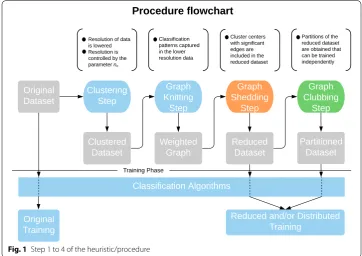
The heuristic procedure organically divides into the following steps:

• Step 1: Clustering step • Step 2: Graph knitting scheme • Step 3: Graph shedding scheme • Step 4: Graph clubbing scheme • Pre-processor for the testing phase

(4)

in two execution modes for the training phase, first in serial mode, and second in dis-tributed mode. Due to an approximate scheme (explained later in the section ‘Graph clubbing scheme’), the serial execution is faster than that of the training on the reduced dataset. Distributed execution can be used to leverage worker threads/processes to get multiple times speed-up. Figure 1 summarizes the steps of the heuristic along with the resulting modifications on the dataset.

Because of the multiple data partitions which translate into as many classifiers, there is a need to determine which classifier to choose for testing a data point. This is achieved by the pre-processor for the testing phase. Lastly, a network application is designed which distributes the obtained partitions in a load-balancing and a communication-free manner.

From a computational point of view, the run-time profile of the first four steps for a typical run case ( n≈100k,d=2,nc≈350 ) is,

• Clustering step takes ≈750 ms or > 98%

• Graph knitting scheme takes ≈10 ms or 1%

• Graph shedding and graph clubbing schemes take ≈2 ms ( <1%)

On the other hand, the pre-processor for the testing phase takes ≈ 5% of the testing phase

time. The clustering step is predominant over subsequent steps with a run-time complex-ity in n, whereas that of all the other steps is in the order of number of clusters ( nc ). The

input parameter to the clustering step, nc , controls the granularity of data representation.

Typically, the ratio of n to nc , which is also known as nominal VC dimension, is 10 to 300,

explaining the run-time dominance of the clustering step. The graph knitting scheme becomes the most computation-intensive among the subsequent steps, because it involves

(5)

heavy space searching. It is to be noted that the run-time percentage profile can vary a lot depending on the nominal VC dimension or the input parameter nc..

Clustering step

The clustering step is used to lower the resolution of the underlying data. In principle, the presented heuristic does not require this step. However, it is not computationally feasible to execute the subsequent steps with a run-time complexity in n instead of nc .

Additionally, it will also affect the generic applicability of the heuristic, which is dis-cussed later in the ‘Graph shedding scheme’ step.

The step consists of a standard K-means++ [25] clustering algorithm, and a metric to store classification patterns of the original data. K-means++ provides improved initial seeding of clusters over the traditional K-means method. This choice leads to running the clustering algorithm for a nominal number of iterations, typically 5. In the current implementation, every cluster center maintains the target class through the weighted average calculation over all its data points. However, advanced metrics can be con-structed to unearth more characteristics of patterns from the clustered data.

Although this step serves only for coarsening the data representation, it dominates the computation cost of the first four steps. Two state-of-the-art K-means++ imple-mentations were tested, K-MeansRex [26] and the scalable mlpack package [27]. For a test run with data points in the range of 1 to 100k ( d=2,nc=100 ), K-means++ from mlpack was 1.82 times faster on average in execution than K-MeansRex’s implementa-tion. Therefore, K-means++ from mlpack is chosen as the standard clustering algorithm in this work.

Given the vast research literature available for clustering methods, there are more advanced implementations available. One of such improvements would be the scalable K-means++ by Bahmani et al. [28], which is shown to be considerably faster than native K-means++. Another practical option is to exploit K-means implementations from a proven distributed computing platform [29].

Graph knitting scheme

(6)

An information graph is constructed once a reasonable representation of the under-lying data is obtained. Two major challenges include determination of neighbors, and capturing the classification patterns in edge weights. First, neighbors are determined such that the whole hypothesis is covered while passively enforcing regularity and planarity in the graph. The neighbors are determined in two steps, followed by a step that controls skewness of the graph. Second, a two-fold pattern capturing edge weight scheme is presented in Eq. 2.

The first challenge of neighbor determination is addressed in two stages, superficial neighbor search (SNS), and exclusive neighbor search (ENS), presented in Part I, and II, respectively. In the algorithm, the number of neighbors is nominally controlled by an input parameter nn, the number of desired neighbors. For every ith node, the vari-able no_tot_neigh[i] in Line 1 of Part I is used to track the size of the neighbor list.

However, the neighbor list for the ith node can be terminated before adding nn neighbors by updating the variable neigh_list_finish[i] to TRUE in Line 4 of Part I. By limiting the number of neighbors in this way, construction of the graph can be controlled.

Part I is used to look for nn nearest neighbors, regardless of the target class. The algorithm takes an empty graph G(V,φ) as input, which is formed with the set of

the cluster centers V after the clustering step. This set is the search space passed to the FLANN space indexing utility in Line 8 and 9. The input constant R is explained later in Eq. 1. Objective of the part is to fill the graph G with EI set of edges. This

is similar to the construction of a K-nearest neighbor graph (K-NNG). However, an input parameter, MAX_SAME_CLASS_NEIGH, is used to limit the number of same class neighbors in Line 13, so that the remainder of edges for the ith node,

nn−no_tot_neigh[i] , are constructed for nodes with the opposite target class. Nodes for which all nn neighbors are found will vary depending on characteristics of the data. They will be excluded from the next parts. An additional computation of reach in Line 15 is maintained for every node. The metric presented in Eq. 1 is similar to the Hausdorff distance [19]. The distance utility of FLANN, in Line 10, is used to compute the summation in Eq. 1, whereas a scaling constant (R) controls the reach according to

where R is the scaling constant, ri is reach of the ith node, xi is the position of the ith node, xj is the position of the jth node, and Ni denotes the set of same class neighbors for the ith node.

(1) ri=R×

jǫNi

(7)

In order to capture the classification patterns completely, it is necessary to make edges along the hypothesis of the classification data. So, Part II extends neighbor searching exclusively for nodes of the opposite target class. The ith node is considered only if there

(8)

Inclusion of a neighbor after space searching in Line 5 is stringent compared to SNS. An input parameter, NEIGH_LIMIT and the computed reach are used to limit the availability of node j as prospect neighbor in Line 9. For every jth node added as a neighbor, the variable node_neigh[j] , initiated in Line 6, is incremented. Reach is used to further update the boolean neigh_list_finish[i] for node i, even if nn−no_tot_neigh[i]>0 in Line 13. Such an ith node tends to be an internal node of a target class. In other words, reach only encourages the convex hull nodes of one class to choose neighbors with nodes of the opposite class, aiding in planar construction of the graph.

The node_neigh counter is required in Part II to avoid a node that might habitually come up as a prospect neighbor despite not being very representative of a target class. It otherwise leads to a skewed graph with respect to node degree. node_neigh in Line 3 of

Part III is used to reduce the search space of every target class, controlling the skewness of the constructed graph.

(9)

target classes. Individual contributions are added via the power scheme in Eq. 2 to weigh the edge according to

where wi,j is the weight of the (i,j)th edge, tc(i) denotes target class of the ith node, CI

and CE are constants for internal and external classification patterns, respectively, and quantities in || are absolute values.

The use of a state-of-the-art implementation like FLANN for neighbor searching can-not be overemphasized. For instance, in a typical run case ( nc>300 and nn>3 ), the

approximate neighbor searching method of FLANN was ≈ 1 000 times faster when

com-pared to the exact algorithm for nearest neighbor searching, which involves computing distances with all the remaining nodes for every node, and then sorting them to deter-mine the nearest neighbors. The run-time advantage is clear when comparing the com-plexity of exact graph construction, O(n3log(n)) , to that of approximate methods offered by FLANN [23].

Graph shedding scheme

Once a weighted graph is obtained, an edge cut based filtering presented in Algorithm 2 separates the training dataset into relevant and non-relevant. For every node, the neigh-bor list is iterated to check for a significant edge in Line 5, and when found, that node is added to relevant_node_list in Line 11. This leads to a training set selection that the second type of approach aims to achieve. Note that the result of this step depends on the characteristics of the graph, such as how well connected the graph is, and how well the underlying classification patterns have been captured. Algorithm 1 with the edge weight scheme addresses these issues.

The role of nominal VC dimension drips down to the pruned graph as well. Since it controls the granularity of the underlying data, it also controls the granularity of data selection. That gives the heuristic an essential advantage in terms of limiting data shrink-age while selecting the relevant data points. Because the selection is done via clusters,

(2)

(10)

and the ratio of n to nc is typically >10 , many data points that are not very close to the

hypothesis boundary of the classification patterns are also selected. That gives an extra buffer of data points upon which another selection method of both types applies. The majority of classification algorithms, for example neural methods, gaussian processes et cetera, can use the heuristic. Until this step, the presented heuristic’s aim matches with the existing approaches of the first and second type. For comparison purposes, the heu-ristic until this step (including) is referred to as GSH for the remainder of this work. Edge cut for GSH is referred to as GS edge cut.

Graph clubbing scheme Formulation

This step extends the problem statement of training set selection to further break-ing the reduced trainbreak-ing set into few partitions or critical chunks, each of which can be trained independently, by virtue of Part I to III of Algorithm 3. The main aim is to design an approximate formulation that is theoretically faster, even for serial execu-tion. The algorithm divides the training set into few partitions such that the number of computations are reduced significantly in the training phase. Consider that the order of complexity of most of the classification algorithms is higher than linear, that is a>1 if O(na) is the complexity. The graph clubbing scheme doesn’t change the order,

how-ever it results in significant reduction in total computations. For example, for a classifi-cation algorithm with O(n2) complexity, if C×n2 , where C is a constant, is the original number of computations; then after data reduction by the graph clubbing scheme, there are four equal sized partitions/critical chunks. Now the number of computations is C×(4×(n₄)2)=C×n₄2 or a quarter of the original number.

Independence during the training phase of each obtained partition is mainly accom-plished because of the directional aspect of the algorithm, which is achieved via the edge weight scheme. The directional aspect is responsible for two objectives, namely obtain-ing equally-sized partitions, and ensurobtain-ing orthogonality of the hypothesis boundary with neighboring partitions’ boundary. Two ways in which the edge weight scheme is lever-aged for the directional aspect is in the priority aspect of the partial weighted matching (PWM) algorithm, Part I, and the reassessment aspect of the coarsening formulation, Part II. The graph clubbing algorithm, Part III, ties Part I, and II in an iterative scheme. Each of such obtained partitions can now be trained independently, giving further lever-age for a nominal number of worker processes.

(11)

reside. Higher prediction accuracies are obtained because of the preference of contraction of the heaviest edges.

The coarsening formulation of Part II applies the directional aspect, as edge contrac-tion occurs in this part. It is to be noted that the coarsening formulacontrac-tion is different in aim to otherwise researched formulations. Most of the popular formulations are intended for reducing communication cost or preserving the global structure while getting a low-cost representation of data [30]. Furthermore, unlike Kernighan-Lin and other matching based coarsening objectives, the presented optimization objective is deterministic in execution.

In the part, reassessment of target class and edge list for newly contracted nodes in Lines 6 and 10, respectively, augments the standard coarsening step in Line 3. By using different values of CI and CE for initial versus reassessment edge weights, the precedence of the kind

of edges is established in the matching scheme. Original heavy edges are prioritized over re-assessed edges of newly contracted edges, achieving the orthogonality property. Transition of coarsening from original edges to newly contracted nodes can be captured by the virtue of drastic decrease in graph cost metric, presented in Eq. 3,

where cost(G) is cost of the graph G, e is an edge, E′ denotes the subset of E (set of all edges) such that {e|eǫEand >EDGE_CUT} , and we is the weight of edge e.

One technical choice is to use MIN(i, j) in Line 4 for identifying the new node that is a result of the contraction of edge between nodes i and j.

(3) cost(G)=

(12)

Part I and II are executed in the iterations of Part III in Lines 5 and 6, respectively. In Line 7, kink detection in graph cost is used as a termination condition of the itera-tive algorithm. However, a variable for the number of coarsening iterations, i.e. MAX_ NUM_OF_COARSENING_ITER in Line 4, is used in the majority of tests. This step concludes the formulation of the heuristic. It is referred to as GCH for the remainder of this work. Similarly, edge cut is referred to as GC edge cut.

(13)

Network design

An event-driven, multi-process algorithm is designed to distribute the partitions obtained after GCH in a communication-free manner. In the network applica-tion, processes assume a (single) master or (multiple) worker role. Part I and II of Algorithm 4, respectively, describe master’s and worker’s side of the event-handling design.

For the master process which executes Part I, one partition from the list of parti-tions, parts_list[] , is communicated to the requesting worker process (the one which

(14)

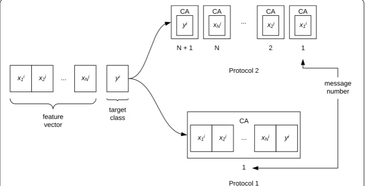
Instead of directly using TCP channels for message communication, the distrib-uted messaging API ZeroMQ [31] is used. It provides essential safety and liveness properties on network channels. However, apart from message guarantees such as the liveness and safety property of ‘once only message delivery’, ZeroMQ is rudimen-tary compared to higher level message passing libraries. This gives an opportunity to design and optimize various aspects of the architecture. One such aspect is the messaging protocol. A couple of messaging protocols are designed as shown in Fig. 2. Protocol 2 implements a single float/double entry (in character array or CA) messag-ing scheme, whereas protocol 1 first requires marshalmessag-ing all entries of a data point before messaging it.

Another aspect that was tested is connection time of the network. Connection time is measured on the master process, and included the following steps:

• Start of TCP channels (wrapped in the API) • Initialize a hash table

• Receive connection request from all worker processes • Send connection confirmation to all worker processes

The connection procedure requires step 2 for maintaining worker processes’ informa-tion, giving an opportunity to optimize the step as required. A light-weight hash table ( ≈0.6 MB) and hash key is designed which generates unique keys. The design helps to reduce the overhead of starting and running the multi-process application.

Pre‑processor for the testing phase

Unlike the application of GSH, which results in a single training set, multiple data partitions are obtained after GCH, and the training set is the union of these parti-tions. It means that there would be as many classifiers as the number of partiparti-tions. Hence, it is needed to determine which classifier to choose for predicting a point

(15)

from the testing dataset, VT . Algorithm 5, nearest hypothesis search (NHS), is used

for this task. A search space is formed consisting of nodes of the coarsened graph in Line 1. ANN search for the nearest hypothesis follows in Line 5.

Once the nearest hypothesis is determined, prediction of the target class for testing data points follows. This added step before the testing phase only takes about 5–7% of the run-time of the testing phase for the SVM class of algorithms, as will be shown in the ‘Results’ section.

Results

Results are presented in two major parts, first with tests on parameter space of the heu-ristic, and second for gauging performance of the heuristic. All the tests were conducted on a variety of datasets.

0.0 0.2 0.4 0.6 0.8 1.0

Feature 1 0.0

0.2 0.4 0.6 0.8 1.0

Fe

ature

2

Class 1 Class 2

(16)

Parameter space of heuristic

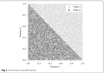
In this set of tests, the focus is on working details, and exemplifying steps of the heuris-tic. Datasets similar to that shown in Fig. 3, with parameters summarized in Table 1, are extensively used.

Node reach and ENS

Tests in this section present heuristic tools that capture original classification data into the weighted graph. These tools are designed to handle real datasets, which vary diversely in characteristics. A mix of real and synthetic datasets that mimic varying characteristics is considered.

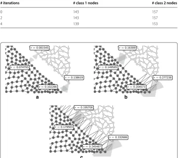
A timeline of the ENS procedure with nn=4 is presented in Fig. 4. It is based on the

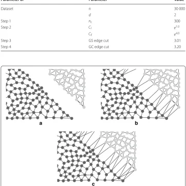
dataset of Table 1. However, class 2 data points were intentionally translated to cre-ate separation, which is very typical for real data. It is evident that the connectivity of the graph increases with more iterations. Skewness control of the constructed graph, Table 1 Dataset along with steps parameters

Parameter of Parameter Value

Dataset n 30 000

d 2

Step 1 nc ₃₀₀

Step 2 CI e1.0

CE e4.0

Step 3 GS edge cut 3.01

Step 4 GC edge cut 3.20

a b

c

(17)

explained in Part III of Algorithm 1, was carried out at end of the iterations of the ENS procedure, resulting in reduction of available nodes for search as shown in Table 2.

A second way to control connectivity is fine tuning of the reach equation, presented in Eq. 1. In the next test, the scaling constant R is varied, and results are presented in Fig. 5. Three cases are shown in succession, under-reach (a), ideal-reach (b), and over-reach (c). Even in the overreach case, inner nodes are not able to make opposite class neighbors, enforcing planar construction of the graph.

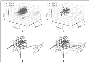
The ENS procedure was next run on a real dataset, called cuff-less blood pressure esti-mation dataset, from the UCI machine learning repository [32, 33]. It is a three attribute, 12 000 instances, real, multivariate dataset. Results are presented in Fig. 6, with subfig-ure (a) showing the dataset, (b) showing cluster centers, whereas (c) and (d) showing the constructed graph without and with ENS procedure, respectively. The latter graph is connected because necessary edges are present between opposite class nodes, cover-ing the entire hypothesis. Class imbalance is analysed next, and results are presented in Table 3. Column 2 shows the number of data points for each class originally, and Col-umn 3 shows the number of data points after ENS, as presented in the graph of Fig. 6d. Imbalance of target classes, quantified by standard deviation (SD), is significantly reduced after ENS.

Table 2 Search space reduction

# iterations # class 1 nodes # class 2 nodes

0 143 157

2 143 157

4 139 153

r = 0.074793

r = 0.081545

r = 0.102286

r = 0.138619

r = 0.149585

r = 0.16309

r = 0.204573

r = 0.277238

r = 0.179503

r = 0.195708

r = 0.245487

r = 0.332686

a b

c

(18)

GSH

The aim of this test is to exemplify the twofold edge weight scheme, shown in Eq. 2. It shows the role of edge weights in the outcome of GSH, summarized in Fig. 7. As clas-sification patterns in the underlying data gets more confused in succession in Subfigures (a) and (c), more edges are weighted significantly, resulting in the selection of a bigger training set by GSH.

GCH

This test exemplifies the formulation of the graph clubbing scheme. Although the edge weight scheme is important in the application of GSH, it is primarily designed to play a crucial role in the priority/directional aspect of the coarsening objective. Constants for initial edge weights were such that CE was kept significantly higher than CI , as shown in

Table 4. Two cases of re-assessments were considered, namely case I and case II. Since initial constants were kept significantly higher than their re-assessment coun-terparts, original nodes were contracted first in both cases, as can be seen in Fig. 8a, b. Transition to contraction of re-assessed type nodes is reflected in the graph cost characteristic in Fig. 9 for case I. After the 2nd iteration, the slope magnitude decreases

Feature 1 2 0

4 6 8 10 Feature 2 0 2 4 6 8 10 Fe_ature 3 0 2 4 6 8 10 Class 1 Class 2

Feature₁4 2 ₀

6 8 10 Feature 2 0 2 4 6 8 10 Fe_ature 3 0 2 4 6 8 10 Class 1 Class 2 a b c d

Fig. 6 Graph knitting procedure. Scaled UCI dataset, clustered data, constructed graph with no and 1 ENS iteration in a–d, respectively. Dashed edges in d are formed after ENS procedure

Table 3 Class imbalance

Procedure # class 1 points # class 2 points SD

None 1743 10,256 4256.5

(19)

significantly because of contraction of all original nodes that have significantly higher edge weights dictated by heavier initial constants. Edge contraction continues to aggres-sively club the graph for case I, including the re-assessed nodes. This results in fewer partitions compared to case II in Fig. 8b. Clubbing is almost shut off in case II because of trivial re-assessment constants. Note that in general, the more coarsening iterations, the fewer partitions.

0.0 0.2 0.4 0.6 0.8 1.0 Feature 1

0.0 0.2 0.4 0.6 0.8 1.0

Feature

2

Class 1 Class 2

0.0 0.2 0.4 0.6 0.8 1.0 Feature 1

0.0 0.2 0.4 0.6 0.8 1.0

Feature

2

Relevant node Non-relevant node

0.0 0.2 0.4 0.6 0.8 1.0 Feature 1

0.0 0.2 0.4 0.6 0.8 1.0

Feature

2

Class 1 Class 2

0.0 0.2 0.4 0.6 0.8 1.0 Feature 1

0.0 0.2 0.4 0.6 0.8 1.0

Feature

2

Relevant node Non-relevant node

a b

c d

Fig. 7 Reduction of training set. Classification data is more confused in (c) compared to (a). b, d show cluster nodes that were selected for (a) and (c) cases, respectively

Table 4 Pattern measure constants of Step 2

Parameter Initial Re‑assessment

Case I Case II

CI e e1.5 1

(20)

Performance evaluations

Several tests were conducted to evaluate performance of the presented methods, includ-ing GSH, serial GCH, and distributed GCH. In addition, the network architecture for distributed GCH is evaluated.

Dataset I was a synthetically constructed two-dimensional, near-linearly separable dataset with parameters shown in Table 5. Dataset II was a similar dataset, but in place of a (nearly) straight-separating hyperplane, a spherical separating hyperplane of radius 0.2 was employed. Otherwise, it uses the same parameters as Dataset I. A dataset from the UCI machine learning repository, called skin segmentation dataset [33, 34], is the next dataset, called Dataset III for the remainder. This classification dataset has four numeric features, and ≈245k observation instances. The nominal VC dimension is 245.

Table 6 summarizes other relevant parameters.

0.0 0.2 0.4 0.6 0.8 1.0 Feature 1

0.0 0.2 0.4 0.6 0.8 1.0

Feature

2

0.0 0.2 0.4 0.6 0.8 1.0 Feature 1

0.0 0.2 0.4 0.6 0.8 1.0

Feature

2

a b

Fig. 8 Partitioning of training set. Number of coarsening iterations is 2 and 10 for (a) and (b), respectively. In each subfigure, the first plot is for the re-assessment case I, whereas the overlaying plot with shifted origin is for case II

0 2 4 6 8 10

Number of iterations 104

105

cost

(

G

)

(21)

An unstructured text dataset from the zenodo public repository is referred to as Data-set IV. This e-commerce dataData-set consists of the title and description of products for four categories, out of which two categories, electronics and clothing are considered, and fea-ture extraction methods including term frequency-inverse document frequency (tf-idf) and word2vec [35] were applied. Parameters of the dataset and steps, along with feature engineering details, are summarized in Table 7. Lastly, an image dataset consisting of Table 5 Dataset I and II along with steps parameters

Dataset Range of # data points

Testing 3–600k

Training 1–200k

d 2

Step 1 # clustering iterations 5

Range of nc 10–400

Step 2 nn 4

# ENS iterations 0

R 0.0–2.0

Step 4 # coarsening iterations 10

GC edge cut 3.10

Table 6 Dataset III along with steps parameters

Dataset Range of # data points

Testing 122,529

Training 122,528

d 3

Step 1 # clustering iterations 5

nc ₅₀₀

Step 2 nn 5

# ENS iterations 0

R 1.0

Table 7 Dataset IV, and test 1 and 2 parameters

Parameter of Parameter Test 1 Test 2

Dataset # of data points 19,226 9613

Feature extraction tf-idf word2vec

Training/total ratio 0.75 0.75

Classification algorithm Tensorflow CNN LIBSVM

Step 2 CI e1.0 e1.0

CE e3.0 _e4.0

(22)

two categories, apparels and speakers, from the zenodo public repository is referred to as Dataset V, on which a VGG16 [36] neural network is applied to get features vectors. Other parameters for this dataset are summarized by Table 8.

Note that the computation setup was kept consistent. Programming language of all codes for which computation time was measured is C/C++. That includes every step of the presented heuristic, and the classification algorithms. Lastly, time stamping was car-ried out on an otherwise idle system.

GSH

The main aim of the following set of tests is to compare the training phase using GSH against the state-of-the-art shrinking heuristics of LIBSVM. Classification algorithms used in these tests were all variants of LIBSVM’s SMO implementation [10], which is a method of the second type.

Two testing variables are evaluated. First, computation run-time of GSH along with the classification algorithm on reduced training data is compared against that of the same classification algorithm but augmented with the shrinking heuristic. Second, Table 8 Dataset V, and test 3 parameters

Parameter of Parameter Test 3

Dataset # of data points 6668

Feature extraction VGG16

Training/total ratio 0.75

# features 25 088

Classification algorithm LIBSVM

Step 1 nc 166

Step 2 CI e1.0

CE e4.0

LIBSVM Training time (sec) 328.39

GSH/Speed-up 70.51/4.7

LIBSVM Prediction accuracy (%) 99.16

GSH 99.16

1k 20k 50k 100k 200k

Number of training data points 0

5 10 15 20 25

Computation

time

(seconds)

LIBSVM shrinking heuristic GSH

SVM training (post GSH)

3k 60k 150k 300k 600k Number of testing data points 98.0

98.5 99.0 99.5

Accuracy

(%)

a b

(23)

the prediction accuracy of the learned models obtained from both the above setups is compared.

Results are presented in the following way. Each of Figs. 10, 11, 12, 13, 14, 15, 16, 17

and 18 is for a SVM classifier, that includes C-SVM and nu-SVM with linear, polyno-mial, and rbf kernels. Subfigure (a) is used to present computation run-time results, and (b) is used for prediction accuracy comparison. Training dataset size was geo-metrically varied from 1k to 200k, and testing dataset size was kept three times that of the training. Accordingly, the parameter nc was varied geometrically in the range

given in Table 5. Note that training time is included in ‘LIBSVM shrinking heuristic’ and ‘GSH’ plots in Subfigure (a), but is not explicitly written for convenience. So the

1k 20k 50k 100k 200k

Number of training data points 0 20 40 60 Computation time (seconds)

3k 60k 150k 300k 600k Number of testing data points 95 96 97 98 99 Accuracy (%)

a b

Fig. 11 C-SVM with polynomial kernel

1k 20k 50k 100k 200k

Number of training data points 0 200 400 600 800 Computation time (seconds)

3k 60k 150k 300k 600k Number of testing data points 98.25 98.50 98.75 99.00 99.25 99.50 Accuracy (%)

a b

Fig. 12 nu-SVM with linear kernel

1k 20k 50k 100k 200k

Number of training data points 0 200 400 600 800 Computation time (seconds)

3k 60k 150k 300k 600k Number of testing data points 92

94 96 98

Accuracy

(%) _{LIBSVM shrinking heuristic}

GSH

a b

(24)

‘GSH’ plots include the run-time of Step 1 to 3 of the heuristic along with the training phase. A third line-plot denoted ‘SVM training (post GSH)’ is presented in Subfigure (a) to separate computation run-time of GSH from subsequent training.

C-SVM with linear kernel was the first classification algorithm tested, as presented in Fig. 10. The GSH scales even for a low number of points ( ≈10k ), as shown in

Sub-figure (a), however, scaling becomes more evident with more training data points. 1k 5k 10k 15k 21k

Number of testing data points

0.0 1.0 2.0 3.0

Difference

in

accuracy

(%)

RS SRS GSH

Fig. 14 Difference in prediction accuracies from LIBSVM for the approaches

0.2 0.3 0.4 0.5 0.6 0.7 0.8 Sampling fraction

0.0 0.2 0.4 0.6 0.8

Computation

time

(seconds)

SRS on case 1 GSH on case 1 SRS on case 2 GSH on case 2

Fig. 15 Compound performance gains from applying GSH after SRS

1k 20k 50k 100k 200k

20 40 60 80 100

Computation

time

(seconds)

3k 60k 150k 300k 600k Number of testing data points 87.4

87.6 87.8 88.0

Accuracy

(%)

a b

(25)

Furthermore, it is visible that GSH took a small fraction of total time, as indicated by the separation between the second and third line plot. It highlights the scalability issue of the SVM formulation. In Subfigure (b), the prediction accuracy of reduced training closely follows that of full training, clearly visible after ≈20k testing data points.

C-SVM with polynomial kernel was the second classifier tested, as presented in Fig. 11. Observations here follow that of the earlier case. Although, one noticeable difference is a better time profile compared to the previous case. This is because of the higher run-time complexity of the polynomial kernel classifier compared to that of the linear kernel presented in Fig. 10.

For the second SMO implementation, nu-SVM, Figs. 12, and 13 summarize linear and polynomial kernel cases, respectively. Note that the training phase with nu-SVM in Figs. 12a and 13a is significantly slower compared to C-SVM in Figs 10a and 11a. Furthermore, it is observed that reduced training can result in improved prediction accuracy, as can be seen in Fig. 13b. For the polynomial kernel, GSH performed better than native training by about 6%.

The next set of two tests emphasize the consistent observation of better prediction accuracy observed for GSH. Given that sampling is a part of GSH, two sampling meth-ods, simple random sampling (SRS) and reservoir sampling (RS) (in the context of big data tool Apache Hadoop [37]), as commonly used in the field of big data, are considered.

In the first test, the sampling size for the two methods is kept the same as the reduced training set size obtained after GSH. Findings are reported in terms of the difference in

1k 20k 50k 100k 200k

Number of training data points 0 20 40 60 Computation time (seconds)

3k 60k 150k 300k 600k Number of testing data points 35 40 45 50 Accuracy (%)

a b

Fig. 17 nu-SVM with linear kernel

1k 20k 50k 100k 200k Number of training data points 0 100 200 300 400 500 Computation time (seconds)

3k 60k 150k 300k 600k Number of testing data points 98.5 99.0 99.5 100.0 Accuracy (%)

a b

(26)

prediction accuracy from LIBSVM, and presented in Fig. 14. It can be seen that GSH exhibits near 0% accuracy difference compared to other approaches. This consistent observation is attributed to the edge weight scheme (applied in the graph knitting step or Step 2) which captures all the classification patterns. In a sampling method of any type, some data points which are important with respect to the classification task are bound to be lost because of the involved stochastics.

In the second test, GSH was applied on the sampled data from the SRS method, for which the sampling fraction was varied from 0.2 to 0.8 for a set of two datasizes, 30 146 and 14 142. The cases are referred to as 1 and 2, respectively, in the computation time results presented in Fig. 15, which are averaged over 10 runs. Table 9 summarizes the prediction accuracy discrepancies of the sampling method from LIBSVM in Column 2, and that of GSH from the sampling method in Column 3. With only compromising

1/3rd to 1/2 confidence in the prediction accuracies, as evident by comparing Column 4

and 5, compound performance gains shown in Fig. 15 can be leveraged.

Dataset I was used in all the tests until now, and near-perfect accuracy plots support that it is an ideal dataset. A more realistic case, Dataset II, was considered for Figs. 16, 17 and 18.

Again, C-SVM with linear kernel was the first classification algorithm tested, as pre-sented in Fig. 16. However, prediction accuracies are in a lower range than before, as shown in Subfigure (b). Nevertheless, both setups are practically identical in pre-diction accuracy. Similar run-time improvements are observed in Subfigure (a). For nu-SVM with linear kernel, presented in Fig. 17, scaling observations are similar to the corresponding Fig. 12, which used Dataset I. Note that the prediction accuracies are only about 50%, which is the expected value for random selection between two target classes. However, note that the main argument here is not the absolute predic-tion accuracy, rather the closeness of it for both setups. To improve the predicpredic-tion Table 9 Results on prediction accuracy

Case Average prediction accuracy ( |%|) Average SD

LIBSVM‑SRS SRS‑GSH LIBSVM‑SRS SRS‑GSH

1 0.006 0.002 0.007 0.003

2 0.087 0.024 0.066 0.028

a b c d e f

0.00 0.02 0.04 0.06 0.08 0.10 0.12 0.14

Computation

time

(fraction)

GSH

(27)

accuracy, results were obtained for a radial basis function (rbf) kernel, which is widely considered a robust kernel type in SVM classifiers, and are presented in Fig. 18. This resulted in slower learning, as observed in Subfigure (a), but near perfect prediction accuracy, as shown in Subfigure (b).

The next set of tests was conducted on Dataset III, for evaluating the performance of the heuristic on real data, and barplots in Figure 19 are used to present the find-ings. Computation run-time was scaled to accommodate different classification algo-rithms, namely C-SVM and nu-SVM with linear, polynomial, and rbf kernels. For all six cases, reported prediction accuracy is low, as shown in Table 10, but close for both setups. Scaling improvements are consistent to the previous reportings for Dataset I and II.

The next set of two tests was conducted on Dataset IV, for evaluating the performance of the heuristic on high-dimensional real data where various feature extraction methods including term frequency-inverse document frequency (tf-idf) and word2vec [35], clas-sification algorithms including CNN from Tensorflow [38] and LIBSVM, dataset size, and dimensions were varied, as summarized in Table 7.

In the first test, use of tf-idf to compute feature vectors resulted in dimensions more than 10k, and the classification algorithm was CNN from Tensorflow [39]. Dataset size Table 10 Prediction accuracy (%)

Classification algorithm LIBSVM GSH

C-SVM

Linear 58 58

Polynomial 58 58

Radial 59 59

nnnu-SVM

Linear 52 58

Polynomial 58 57

Radial 55 48

Table 11 Test parameters and results

Fraction of #

data points # features

nc Training time (seconds) Prediction accuracy

(%)

Tensorflow GSH (/speed‑up) Tensorflow GSH

0.2 10,621 96 2603.82 1201.11 /2.2 98.54 98.45

0.5 15,613 240 11,851.98 1664.38 /7.1 99.13 99.13

Table 12 Test parameters and results

word2vec input

dimension Training time (seconds) Prediction accuracy (%)

LIBSVM GSH (/speed‑up) LIBSVM GSH

500 100.88 12.06 /8.3 98.04 98.79

(28)

was the variable, and results are presented in Table 11, from which scaling advantages of GSH without change in prediction accuracy are apparent. In the second test, a state-of-the-art feature extraction method, word2vec, was applied to generate the vectors for a set of two dimensions, 500 and 1 000, which were then used to train a LIBSVM classifier with linear kernel. It is apparent from the results presented in Table 12 that a speed-up of ≈10 can be achieved with 0.77% improvement in average prediction accuracy.

Similar to the previous two tests, the last test was conducted on Dataset V, where the feature extraction method of VGG16 [36] and LIBSVM classifier with linear kernel was used, along with other parameters summarized in Table 8. Results are presented in the last four rows of the table, which shows that a speed-up of 4.7 times can be achieved over more than 25k features without compromising any prediction accuracy.

Overall, scalability improvements are observed consistently over a number of classi-fiers for Dataset I to V. Furthermore, the prediction accuracy either closely follows origi-nal training or even outperforms it in a few instances.

Serial GCH

The next set of tests are aimed to compare run-time of serial GCH to that of GSH. More precisely, serial execution of GCH, which represents approximate learning, is fared against (reduced training data) GSH learning. In GCH, the graph clubbing step was an added cost over GSH, so the ‘GCH’ plots include the run-time of Step 1 to 4 of the heu-ristic along with serial execution of the training phase for the obtained partitions (after Step 4). Results are presented for Dataset I.

The number of iterations was set 10, and used as the termination condition for the graph clubbing algorithm. The pre-processor was used, and the collected prediction accuracies were weight-averaged over all reported partitions. Edge weight constants given in Table 13 were used throughout.

Table 13 Pattern measure constants (of Step 2) for GCH

Parameter Initial Re‑assessment

CI e e1.5

CE e5 1

1k 20k 50k 100k 200k

5 10 15 20 25

Computation

time

(seconds)

LIBSVM shrinking heuristic serial GCH

GSH

3k 60k 150k 300k 600k Number of testing data points 95

96 97 98 99

Accuracy

(%)

LIBSVM shrinking heuristic serial GCH

a b

(29)

Only GSH and GCH are compared along with respective line-plots of subsequent training for all the classifiers, as presented in Figs. 22 and 23. However, for the first classifier, C-SVM with linear kernel, shown in Fig. 20, computation run-time of

1k 20k 50k 100k 200k

1 2 3 4 5

Numb

er

of

critical

chunks

Fig. 21 Partitions after GCH

1k 20k 50k 100k 140k

2 4 6 8 10 12 14

Computation

time

(seconds)

serial GCH

SVM training (post GCH) GSH

Fig. 22 C-SVM with polynomial kernel

1k 20k 50k 100k 200k

2 4 6 8

Computation

time

(seconds)

serial GCH

SVM training (post GCH) GSH

(30)

LIBSVM with shrinking heuristic is also plotted. An accuracy plot, Subfigure (b), and a plot for the number of partitions in Fig. 21 are also presented.

In Fig. 20a, a clear scalability hierarchy is observed, with serial GCH > GSH > LIBSVM shrinking heuristic. In the accuracy plot, shown in Subfigure (b), approximate learning closely follows native learning for more than 8k training data points. However, for fewer points, the accuracy of the model trained after GCH, which is ≈ 95%, is not as good as

native training at 99% . 2 to 5 partitions were obtained as shown in Fig. 21. For

polyno-mial kernel classifiers, presented in Figs. 22 and 23, scaling advantages with serial GCH compared to GSH are observed even for fewer data points ( ≈5k).

Distributed GCH

The main aim here was to demonstrate run-time advantages with worker processes for the communication-free training scheme discussed earlier. The plots here differ from ‘serial GCH’ plots only by the mode of execution of the training phase, that is, obtained partitions are distributed to worker processes as per the network design or Algorithm IV. The scheme only aims for coarse grain parallelization, such that indi-vidual data chunks/partitions can be distributed to worker processes.

0 50k 100k 150k 200k Number of training data points 0.2 0.3 0.4 0.5 0.6 0.7 0.8 0.9 1.0 Computation time (fraction)

# workers : 2 # workers : 3 # workers : 4

1k 20k 50k 100k 200k Number of training data points 0 2 4 6 8 Numb er of critical chunks a b

Fig. 24 Scalability with workers (a), and obtained partitions (b)

1k 10k 100k 200k

Number of training data points 0 1k 2k 3k 4k 5k 6k 7k 8k Average dat ap oint sp er chunk

(31)

Results are presented in Fig. 24 for C-SVM with a polynomial kernel classifier on Dataset I. The distribution invariantly depends on the number of obtained partitions. Therefore, scaling results in Subfigure (a) cannot be interpreted without the plot for the number of partitions, which is shown in Subfigure (b).

Significant improvements are observed with more workers. However, sub-optimal distribution with number of workers more than 2 can be seen in Fig. 25. Mean num-ber of data points per chunk/partition is plotted as a function of the numnum-ber of total data points. Using the number of partitions/chunks from Fig. 24b, it is straightfor-ward to interpret the monotonic increase of the plot. In a hypothetical case where the partitions are all equally-sized, SD would be zero. However, as the number of total data points increases, error bars for SD are observed to be commensurate to the mean number of data points. Unequal size of partitions is the apparent reason for the sub-optimal distribution. Overall, Table 14 summarizes the performance gains for all the approaches, namely GSH, serial GCH and distributed GCH, relative to the shrinking heuristic available in LIBSVM for C-SVM with a polynomial kernel on Dataset I. Table 14 Scaling improvements of the heuristic approaches

# of training

points Shrinking heuristic_{of LIBSVM} GSH serial GCH dist. GCH_{(w/2 proc.)} dist. GCH_{(w/4 proc.)}

(seconds) (× of serial GCH)

1000 0.0078 0.0076 0.0073 1.5 3.0

4543 0.0604 0.0339 0.0290 1.7 2.3

9686 0.1957 0.0981 0.0631 1.3 1.6

20,647 0.7422 0.2515 0.1359 1.8 2.2

93,823 9.6774 2.3658 1.0003 1.8 3.6

136,984 20.4771 3.9556 1.9835 1.5 2.0

1 2 3 4 5 6 7

Number of workers 0.08

0.10 0.12 0.14 0.16

Connectio

nt

ime

(seconds

)

(32)

Network design

The main motivation for this set of tests was to evaluate various implementation aspects of the network that implemented distributed GCH. The first aspect is the connection time of the distributed application. Fig. 26 shows connection time meas-urements with the number of workers.

Apparently, the connection time is very small ( ≈120 ms ) when compared to the

run-time of the training phase. The connection procedure was replicated on another distributed messaging API, MPICH3.3 [40], and the connection time with ZeroMQ was observed to be 1.53 times faster than with MPICH3.3.

The next aspect of the network is the messaging protocols. The primary motiva-tion behind the protocol design is to utilize the shape of the ith data point, that has

an n-dimensional feature vector ( xi ), and a 1-dimensional target class value (tc(i)) .

Two of such protocols as previously discussed were fared in run-time. A couple of opposing factors are at play between these protocols. Data marshaling is an extra step in protocol 1 (before actual messaging) when compared to protocol 2. On the other hand, message count/traffic increases (multiple times governed by the dimensionality

0 5M 10M 15M 20M

Number of communicated data points 0

4 8 12 16

Computation

time

(seconds)

Protocol 2 Protocol 1

Fig. 27 Evaluation of messaging protocols. Protocol 1 is used in this work

0 1M 2M 3M 4M 5M 6M

Number of testing data points 0

2 4 6 8

Te

sting

run-time

(%)

Messaging Pre-processing

(33)

of data) in protocol 2 compared to protocol 1. Overall, protocol 1 performed bet-ter as can be been in Fig. 27. Although increased marshaling may probably result in even better scaling, a larger memory footprint on the channel is un-advisable as it can result in an overflow scenario.

Messaging efficiency was tested in the context of prediction/testing phase of the distributed implementation. Reported in Fig. 28, it is very efficient at ≈ 1% of the

pre-diction time. It is found to be even more efficient at ≈ 0.5% for the training phase.

Pre-processing run-time is at ≈ 7%, as can be seen in Fig. 28.

Note that external libraries are used in the formulation, including a clustering method, an approximate nearest neighbor implementation, two messaging APIs, and many classification algorithms. The heuristic execution is not very sensitive to the parameters of these external implementations. For instance, only 3–5 iterations of clustering were needed, input parameters for approximate nearest neighbor and clas-sification algorithms were kept at default. However, the heuristic is sensitive to the parameters which are part of the heuristic steps.

Conclusions and future work

In this work, an algorithm with an edge weight scheme is designed to construct a weighted graph that effectively captures the classification patterns of the training data-set. Another graph coarsening algorithm with a directional aspect is formulated that divides the reduced dataset into partitions that can be trained independently using a novel communication-free network.

GSH provides an evident serial scalability advantage, and generic applicability holds for every classifier. Then, approximate learning is the reason behind serial GCH’s added run-time advantage over GSH. Finally, distribution of chunks/partitions (after GCH) of the training set to worker processes results in further run-time improvements in distributed GCH. Overall, for all the approaches, namely GSH, serial, and distributed GCH, scaling benefits against full data training with classification algorithms from LIBSVM and Tensor-flow are accompanied by no compromise in prediction accuracy.

Unequal coarsening and control over the number of partitions still needs to be further investigated in the current implementation of GCH in two possible areas,

• First is the directional aspect of the objective. That is, if the partitioning was better directed, better orthogonality between the contour of the underlying classification pat-terns and of partition boundaries shall be obtained in the approximate procedure. The two-fold pattern measure scheme should be designed to get the desired control over the direction of coarsening.

(34)

Abbreviations

WSS: working set selection; SMO: sequential minimal optimization; VC dimension: Vapnik Chervonenkis dimension; ANN: approximate nearest neighbors; SD: standard deviation; K-NNG: K-nearest neighbors graph; SNS: superficial neighbor search; ENS: exclusive neighbor search; GSH: graph shedding heuristic; GCH: graph clubbing heuristic; NHS: nearest hypothesis search; SRS: simple random sampling; RS: reservoir sampling; n: number of data points; d: number of features; nc: number of initial clusters (input parameter); wi,j: weight of (i,j) edge; tc(i): target class of the ith node; CI: constant for internal classification pattern; CE: constant for external classification pattern; R: reach constant (input parameter); ri: reach

of the ith_node;xi: position of the ith node; xj: position of the jth node; N_i: set of neighbors of ith node; cost(G): cost of graph G_;_e_{: an edge;}E′_{: subset of}_E_{(set of all edges) such that}_{e_|e_ǫEand > GC edge cut}; w_{e: weight of an edge}_e_.

Acknowledgements

SY acknowledges Gautam Kumar’s contributions in the project.

Authors’ contributions

This work is joint research of SY and MB. SY did all implementation, and run all test cases. All authors read and approved the final manuscript.

Funding Not applicable.

Availability of data and materials

Dataset I and II used during the current study are available from the corresponding author on a reasonable request. Furthermore, two real datasets used are available in the UCI machine learning repository, https ://archi ve.ics.uci.edu/ml/ datas ets/skin+segme ntati on. https ://archi ve.ics.uci.edu/ml/datas ets/Cuff-Less+Blood +Press ure+Estim ation . Dataset IV and V are available in the zenodo public repository, https ://doi.org/10.5281/zenod o.33558 23. https ://doi.org/10.5281/ zenod o.33569 17, respectively. Other resources with respect to the manuscript are shared at https ://sumed hyada v.githu b.io/graph _heu/. Tests were performed with following computing specfications: Operating system(s): Ubuntu 16.04 LTS. Programming language: C/C++, python (for visualization). Visualization tools: matplotlib and networkx modules in python. External Libraries: FLANN (1.8.4), mlpack (3.0.4), LIBSVM (3.23), Tensorflow (1.12.0), Keras (2.2.4). Version require-ments: g++ 5.4.0, Python 2.7.12, matplotlib 1.5.1, networkx 2.2, numpy 1.15.4.

Competing interests

The authors declare that they have no competing interests. Author details

1_{Gstech Technology Pvt. Ltd., 415, 2nd Floor, 16th Cross Road, 17th Main Road, HSR Layout Sector 4, Bengaluru 560102,} India. 2_{Institute for Combustion Technology, RWTH Aachen University, Templergraben 64, 52056 Aachen, Germany.}

Received: 5 June 2019 Accepted: 12 October 2019

References

1. Levy AY, Fikes RE, Sagiv Y. Speeding up inferences using relevance reasoning: a formalism and algorithms. Artif Intell. 1997;97:83–136. https ://doi.org/10.1016/S0004 -3702(97)00049 -0.

2. Blum AL, Langley P. Selection of relevant features and examples in machine learning. Artif Intell. 1997;97:245–71.

https ://doi.org/10.1016/S0004 -3702(97)00063 -5.

3. Weng J, Young DS. Some dimension reduction strategies for the analysis of survey data. J Big Data. 2017;4(1):43.

https ://doi.org/10.1186/s4053 7-017-0103-6.

4. Guyon I, Gunn S, Nikravesh M, Zadeh LA. Feature extraction: foundations and applications. In: Studies in fuzziness and soft computing, vol 207. Berlin Heidelberg: Springer, Springer-Verlag; 2008. https ://doi.org/10.1007/978-3-540-35488 -8.

5. Fayed H. A data reduction approach using hyperspherical sectors for support vector machine. In: DSIT ’18:Proceed-ings of the 2018 international conference on data science and information technology, Singapore, Singapore. ACM, New York, NY, USA; 2018. https ://doi.org/10.1145/32392 83.32393 17.

6. Coleman C, Mussmann S, Mirzasoleiman B, Bailis P, Liang P, Leskovec J, Zadaria M. Select via vroxy: efficient data selection for training deep networks; 2019. https ://openr eview .net/forum ?id=ryzHX nR5Y7 . Accessed on 1 Feb 2019. 7. Loukas A, Vandergheynst P. Spectrally approximating large graphs with smaller graphs; 2018. CoRR arXiv :1802.07510 . 8. Weinberg AI, Last M. Selecting a representative decision tree from an ensemble of decision-tree models for fast big

data classification. J Big Data. 2019;6(1):23. https ://doi.org/10.1186/s4053 7-019-0186-3.

9. Chen PH, Fan RE, Lin CJ. A study on smo-type decomposition methods for support vector machines. Trans Neural Netw. 2006;17:893–908. https ://doi.org/10.1109/TNN.2006.87597 3.

10. Fan RE, Chen PH, Lin CJ. Working set selection using second order information for training support vector machines. J Mach Learn Res. 2005;6:1889–918.

11. Nalepa J, Kawulok M. A memetic algorithm to select training data for support vector machines. In: GECCO ’14:Pro-ceedings of the 2014 annual conference on genetic and evolutionary computation, Vancouver, BC, Canada. ACM, New York, NY, USA; 2014. https ://doi.org/10.1145/25767 68.25983 70.

(35)

13. Awad M, Khan L, Bastani F, Yen IL. An effective support vector machines (SVMs) performance using hierarchical clustering. In:16th IEEE international conference on tools with artificial intelligence, p. 663-7; 2004. https ://doi. org/10.1109/ICTAI .2004.26.

14. Cervantes J, Li X, Yu W, Li K. Support vector machine classification for large data sets via minimum enclosing ball clustering. Neurocomputing. 2008;71:611–9. https ://doi.org/10.1016/j.neuco m.2007.07.028.

15. Li X, Cervantes J, Yu W. Two-stage svm classification for large data sets via randomly reducing and recovering training data. In: IEEE international conference on systems, man and cybernetics, October 2007; 2007. https ://doi. org/10.1109/ICSMC .2007.44138 14.

16. Wang J, Neskovic P, Cooper LN. A minimum sphere covering approach to pattern classification. In: ICPR’06:18th international conference on pattern recognition. 2006, 3:433-6; 2006. https ://doi.org/10.1109/ICPR.2006.102. 17. Mavroforakis ME, Theodoridis S. A geometric approach to support vector machine (SVM) classification. Trans Neural

Netw. 2006;17:671–82. https ://doi.org/10.1109/TNN.2006.87328 1.

18. Fung G, Mangasarian OL. Data selection for support vector machine classifiers. In: KDD ’00:Proceedings of the Sixth ACM SIGKDD international conference on knowledge discovery and data mining. Boston, Massachusetts, USA. ACM, New York, NY, USA; 2000. https ://doi.org/10.1145/34709 0.34710 5.

19. Wang J, Neskovic P, Cooper LN. Training data selection for support vector machines. In: ICNC’05:Proceedings of the first international conference on advances in natural computation—Volume Part I, Changsha, China. Springer-Verlag, Berlin, Heidelberg, Germany; 2005. https ://doi.org/10.1007/11539 087_71.

20. Yu H, Yang J, Han J. Classifying large data sets using SVMs with hierarchical clusters. In: KDD ’03:Proceedings of the ninth ACM SIGKDD international conference on knowledge discovery and data mining, Washington, DC, USA. ACM, New York, NY, USA; 2003. https ://doi.org/10.1145/95675 0.95678 6.

21. Chang CC, Lin CJ. LIBSVM: a Library for support vector machines. ACM Trans Intell Syst Technol. 2011;2:27. https :// doi.org/10.1145/19611 89.19611 99.

22. Chau LA, Li X, Yu W. Convex and concave hulls for classification with support vector machine. Neurocomputing. 2013;122:198–209. https ://doi.org/10.1016/j.neuco m.2013.05.040.

23. Muja M, Lowe DG. Scalable nearest neighbor algorithms for high dimensional data. IEEE Trans Pattern Anal Mach Intell. 2014;36:2227–40. https ://doi.org/10.1109/TPAMI .2014.23213 76.

24. Leevy JL, Khoshgoftaar TM, Bauder RA, Seliya N. A survey on addressing high-class imbalance in big data. J Big Data. 2018;5(1):42. https ://doi.org/10.1186/s4053 7-018-0151-6.

25. Arthur D, Vassilvitskii S. K-means++: The advantages of careful seeding. In: SODA ’07:Proceedings of the eighteenth annual ACM-SIAM symposium on discrete algorithms. New Orleans, Louisiana. Society for Industrial and Applied Mathematics, Philadelphia, PA, USA; 2007.

26. Hughes M. KmeansRex : Fast, vectorized C++ implementation of K-Means using the Eigen matrix template library; 2018. https ://githu b.com/micha elchu ghes/KMean sRex. Accessed on 1 Dec 2018.

27. Curtin RR, Edel M, Lozhnikov M, Mentekidis Y, Ghaisas S, Zhang S. mlpack 3: a fast, flexible machine learning library. J Open Source Softw. 2018;3:726. https ://doi.org/10.21105 /joss.00726 .

28. Bahmani B, Moseley B, Vattani A, Kumar R, Vassilvitskii S. Scalable K-means++. Proc VLDB Endow. 2012;5:622–33.

https ://doi.org/10.14778 /21809 12.21809 15.

29. Zaharia M, Xin RS, Wendell P, Das T, Armbrust M, Dave A, Meng X, Rosen J, Venkataraman S, Franklin MJ, Ghodsi A, Gonzalez J, Shenker S, Stoica I. Apache Spark: a unified engine for big data processing. Commun ACM. 2016;59:56– 65. https ://doi.org/10.1145/29346 64.

30. Dhillon IS, Guan Y, Kulis B. Weighted graph cuts without eigenvectors a multilevel approach. IEEE Trans Pattern Anal Mach Intell. 2007;29:1944–57. https ://doi.org/10.1109/TPAMI .2007.1115.

31. Akgul F. ZeroMQ. Birmingham: Packt Publishing; 2013.

32. Kachuee M, Kiani M, Mohammadzade H, Shabany M. Cuff-less high-accuracy calibration-free blood pressure estimation using pulse transit time dataset; 2015. https ://archi ve.ics.uci.edu/ml/datas ets/Cuff-Less+Blood +Press ure+Estim ation . Accessed 1 Dec 2018.

33. Dua D, Graff C. UCI machine learning repository; 2019. http://archi ve.ics.uci.edu/ml. Accessed 1 Dec 2018. 34. Bhatt R, Dhall A. Skin segmentation dataset; 2012. http://archi ve.ics.uci.edu/ml/datas ets/skin+segme ntati on.

Accessed 1 Dec 2018.

35. Řehůřek R, Sojka P. Software Framework for Topic Modelling with Large Corpora. Proceedings of the LREC 2010 Workshop on New Challenges for NLP Frameworks 45-50; 2010. http://is.muni.cz/publi catio n/88489 3/en. Accessed 28 July 2019.

36. Simonyan K, Zisserman A. Very Deep Convolutional Networks for Large-Scale Image Recognition; 2014. CoRR arXiv :1409.1556.

37. Shvachko K, Kuang H, Radia S, Chansler R. The Hadoop Distributed File System, Proceedings of the 2010 IEEE 26th symposium on mass storage systems and technologies (MSST) MSST ’10:1-10; 2010. https ://doi.org/10.1109/ MSST.2010.54969 72.

38. Abadi M et al.. TensorFlow: Large-scale machine learning on heterogeneous systems; 2015. https ://www.tenso rflow .org/. Accessed 27 July 2019.

39. François C et al. Keras; 2015. https ://keras .io. Accessed 27 July 2019.

40. MPICH3.3. A high performance and widely portable implementation of the message passing interface (MPI) stand-ard; 2018. https ://www.mpich .org/. Accessed 1 Feb 2019.

Publisher’s Note