R E G U L A R A R T I C L E
Open Access
Quantifying decision making for data
science: from data acquisition to modeling
Saurabh Nagrecha and Nitesh V Chawla
**Correspondence: [email protected] iCeNSA, Department of Computer Science and Engineering, University of Notre Dame, Notre Dame, IN 46556, USA
Abstract
Organizations, irrespective of their size and type, are increasingly becoming
data-driven or aspire to become data-driven. There is a rush to quantify value of their own internal data or the value of integrating their internal data with external data, and performing modeling on such data. A question that analytics teams often grapple with is whether to acquire more data or expend additional effort on more complex modeling, or both. If these decisions can be quantifieda priori, it can be used to guide budget and investment decisions. To that end, we quantify the Net Present Value (NPV) of the tasks of additional data acquisition or more complex modeling, which are critical to the data science process. We develop a framework,NPVModel, for a comparative analysis of various external data acquisition and in-house model development scenarios using NPVs of costs and returns as a measure of feasibility. We then demonstrate the effectiveness of NPVModel in prescribing strategies for various scenarios. Our framework not only acts as a suggestion engine, but it also provides valuable insights into budgeting and roadmap planning for Big Data ventures.
Keywords: cost sensitive learning; business value; external data
1 Introduction
Organizations are rapidly embracing data science to help inform their decision making and generate an impact in their business or operations, whether it is in increased revenue, reduced costs, or improved efficiencies. To that end, organizations are incorporating an-alytics programs to not only deliver value from their internal data, but also connect their internal data with external data sources to develop a more complete data profile for mod-eling.aAcquiring external data is not cheap and requires an investment from the organiza-tion. Similarly, developing more advanced or complex models may also require investment in people or computational resources. To that end, the analytics teams in organizations may grapple with the following questions:) Can they optimize aspects of the data science process to lower the costs, resulting in a higher overall Return on Investment (RoI)? ) Is there an objective way to compare the value of different strategies — data acquisition or modeling or both?
While there is a paradigm of cost-sensitive learning or budgeted learning, it does not take into account the explicit costs of data acquisition or modeling, and the Net Present Value (NPV) of implementing the overall data science process or the analytics program. This adds a whole new dimension to the problem of implementing and deploying analytics
strategies. For example, an organization switching external data providers would incur upfront costs to switch the data pipeline, potential warehousing, integration into existing model, etc. These concerns are further complicated by the variety of offerings by potential data vendors in terms of features, instances, costs, and delivery model.
Problem statement Given a fixed budget and knowledge of associated costs, this paper aims to answer the following questions:
. Should one invest dollars on external data acquisition or more complex/advanced modeling or both?
. How much money should one invest in external data acquisition? What is a fair price estimate to pay for the expected outcomes?
. What returns should one expect?
. How can one pivot from an existing strategy over time? How should teams and organizations chart a roadmap for the data analytics project horizon?
These questions can form an objective data-driven set of strategies for analytics teams as they consider the cost and impact of analytics programs for an organization. The answers to these questions rely on a deeper understanding of how one acquires external data and how one develops their analytics solutions (modeling).
1.1 Assumptions
We assume that the following costs, or an estimate of them are known beforehand: internal model development costs, external data acquisition costs, opportunity costs, misclassifi-cation costs at each stage, and costs involved with pivoting strategies. These costs can be dynamic and subject to change over the life cycle of the project. If the costs are unknown, then we can use minimum and maximum costs to establish bounds on the final NPV. The cost matrix presented in Section . shows how this is done. One relevant use-case for this would be to help negotiate the price for external data with an external provider.
We do not,a priori, know whether or not a certain external dataset will improve per-formance. Instead, in our approach, we use a standard industry practice — running the model on a pilot external dataset, and then evaluating its performance. In our framework, NPVModel, we take this further and convert it into the NPV of costs for the external (pi-lot) dataset. If the NPV of costs is lowered, then we can say that this external dataset was useful. The generalizability of this relies on the assumption that the pilot data (on which these decisions are made) is indicative of the test data (which is used in practice). Over the course of time, if the external data no longer adds to the performance of the model, then it is clearly reflected in its NPV, which will be greater than or equal to those for a model run without external data.
1.2 Target metrics
A machine learning or statistical model’s performance is evaluated on metrics like accu-racy, precision, recall, Area Under the ROC Curve (AUC),f(β), etc. on the incoming test data; but in order for these to be usable for business decisions, these need to be converted to a dollar value. A static dollar value at a given point in the future needs to be contextual-ized for current considerations. Thus, the NPV of this dollar amount offers a good estimate of that cost, and as a result, the time-value of predictions obtained. This now enables us to compare inherently different strategies head-to-head, solely on the basis of expected re-turns. We refine the question aswhat is the monetary value of a dynamic prediction system over a period of time?
1.3 Contribution
There can be an inherent trade-off between investing resources into external data acquisi-tion and in-house model development. The feasibility of these strategies is evaluated stat-ically, frequently during initial model development. However, a static evaluation fails to take into account the time value of model development. To account for this consideration, our approach is to decouple the considerations regarding acquisition of external data and model development, translate each component’s contribution to monetary returns, and then evaluate the relative strength of an investment strategy.
Our contribution is to propose and develop a recommendation framework, NPVModel, which suggests the best possible business practice for analytics tasks or strategy. In this framework, one can unify costs of model development, external data acquisition, and those of the time value of predictions; this facilitates the development of strategies that derive synergy from the appropriate confluence of model development and external data acquisition.
2 Related work
Since this paper reconciles multiple aspects of machine learning, we provide a brief overview of the relevant techniques in literature from the following sub-disciplines.
2.1 Cost sensitive classification
A survey of cost-sensitive learning techniques over the years is covered in []. Motivated by their popularity, [] focuses on cost-sensitive learning for tree-based classification tech-niques.
These papers evaluate performance by using multiclass datasets from the UCI reposi-tory, associating arbitrary costs with (mis)predictions for each class. These papers demon-strate effective performance by showing that their cost islowerthan the contemporary state of the art.
Cost sensitive learning can be implemented using an inherently cost-sensitive classifica-tion approach, or using a “wrapper” which converts an otherwise cost-agnostic classifier into a cost sensitive one. Popular techniques for inherently cost sensitive classifiers involve minority class resampling, treating thresholds of minority class differently, tweaking the splitting criteria for minority class, pre- and post-pruning of hypotheses, and combina-tions thereof.
Cost Sensitive Naive Bayes [], and Empirical Thresholding [] operate similarly and can be alternatively used as wrappers instead of MetaCost. Other meta-learning wrapper tech-niques such as Costing [] and Weighting [] employ sampling in the training phase and then use cost-agnostic classifiers on the resampled data. Of the two (wrappers and resam-pling), wrapper based meta-learning techniques are easier to integrate into the work-flow of existing solutions.
Our main focus is in the application of cost sensitive methods as part of a broader frame-work, and not the finer workings or comparisons of each of the specific solutions. To that end, we use MetaCost as a representative method from the wrapper techniques discussed above.
2.2 Timeliness of prediction
Cost sensitive classification generally works in a static framework, and does not explic-itly address the timeliness of predictions. Applications require a classification system to perform over the duration of their deployment. Domingos [] considers the feasibility of implementing a cost model for machine learning systems, and illustrates a net-present-value investment-return model until perpetuity. In this paper, we consider a dollar-net-present-value based cost, but it can be easily modified to other cost considerations as well.
2.3 External data acquisition
Another avenue to potentially enhance the business value of a prediction system is to in-corporate external data. However, this often begs the question: is external data acquisition feasible? In order for it to be feasible, external data must provide an increase in perfor-mance, for which it must enhance the discernibility of the classifier. Provost and Weiss have discussed [] the impact of class distribution in the training data on classifier per-formance. This answers the question regardingwhatquality of external data one must aim for, when such data is available at a premium. Transforming machine learning metrics to dollar amounts has been discussed in []. Again, the authors’ treatment of the subject is limited to a static setting. The paper by Weiss et al. [] is one of the few papers to discuss costs of acquiring external data, though it discusses it in terms of a CPU based cost.
2.4 Active learning
In the spirit of labeled instances being available at a premium, the field of active learning has various solutions that must be acknowledged with respect to the NPVModel. Active learners seek out additional data labels at a cost. Cost sensitive active learners can be in-duced as shown in []. Ideas from Proactive learning [] can be incorporated just the same as for active learning. Proactive learning goes beyond some of the assumptions in active learning and relaxes the assumptions that the external ‘oracle’ is always right, al-ways available, alal-ways costs the same to query, or that there is just one oracle. NPVModel applies the concept of time-value of costs to the existing idea of active learning.
Overall, in literature, we see that the problems of model development, external data acquisition, and time value of prediction have been separately addressed, but no singular work ties these concepts together.
3 Proposed framework: NPVModel
pre-dictor is applied to these, and the prepre-dictor is re-trained for the next time interval while including the newly introduced instances. This is the baseline system that predicts out-comes based on new instances. In the process, it predicts some instances correctly, which generate revenue, and it makes some errors, which cost money. The NPV of this base-line model is considered to be the criteria for feasibility. Since all subsequent alternative strategies piggyback on this model, we can set the NPV of this approach to be as that of a
null model— all strategies whose NPV is less thanNPVnullare infeasible, and those whose NPV is greater thanNPVnullare feasible.
Data science or analytics strategies can be characterized in terms of external data ac-quisition and/or model development. The data acac-quisition costs could include the cost of purchasing and integrating new data in to a data science work-flow. The cost of model development can be the human resources expended towards model development as well as possible computational cost. Costs associated with cloud computing servicesbcan be estimated and factored in. Each of these decisions has an underlying investment-return model. Our goal is to best characterize this model in terms of an objective NPV so as to compare vastly differing strategies head-on. Section . discusses several models used for external data investment strategies. Each strategy’s NPV of cost is calculated and the strategy with the highest NPV (i.e. lowest NPVcost) is deemed most feasible. The most feasible strategy is a solution of the form which informs analysts of three parameters:what kindof external data model is the best,what kindof model development is best, andwhen
any/each of these should be deployed, specific to their environment.
3.1 External data acquisition
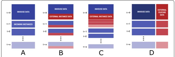
External data can be obtained under three basic models — additional training data in-stances, additional features/attributes or both. This is as illustrated in Figure . In the case of additional instances, one can purchase these all at once, or in batches [, ]. The for-mer is relevant in cases where the external data provider does not update their data at least within the period of the project. In reality, these could be external data sources where it may not even be necessary to update the data sources so long as sufficient external data is available. The latter is reflective of the practice followed by many external data providers, who themselves keep updating their data warehouses with new data instances. We use both models for our experiments where external data instances are added.
To show the various scenarios in which the integration of external data can be imple-mented, we explore the following cases as per Figure :
• Case A: (The basic model) No external data. • Case B: Up-to-date batch-wise external instances. • Case C: One-time external instance dump.
• Case D: External features for each of the in-house instances.
Since up-to-date batch-wise data and one-time-dumps are very different methods to ac-quire external data, caution must be exercised when comparing these strategies directly. So, one can directly compare cases A, B, and D directly and A, C, and D directly. Under equivalent processes of external data acquisition, a direct comparison may be possible, e.g.: providing all national road accident related data as it happens (B), or in the form of a yearly dump (C). This shows that B and C stem from different data-collection timelines, and comparing them is equivalent to comparing an online batched predictor to a “pre-scient” one, which has access to all the data at once.
The set-up of the experiments in this paper is such that each dataset’s prediction task is evaluated with and without various cases of external data. Since we aim to make no assumption regarding the nature of what form the external data can take, it covers each scenario from Section ., viz. Cases A through D. In case of external data instances, the in-stances are only taken into account for model development and not for prediction. In case of external features, the feature values are added to the feature-space of the internal data. This means that upon querying an external dataset with an instance (Xi= (xint,, . . . ,xint,m)), we get a new set of features ((xext,, . . . ,xext,m)), which are added to the feature-space of the internal dataset, resulting in the instanceXi= (xint,, . . . ,xint,m,xext,, . . . ,xext,m).
3.2 Machine learning model development
In-house model development comes with many associated costs. In order to evaluate the RoI of an in-house modeling (analytics) team, we break it down into its two components: the investment (the salaries and upkeep costs) and the returns (the difference in NPV of predictive performance). We set forth tiers of costs-to-company for certain in-house modeling costs. These costs are merely estimates of how much overall investment has gone into development, and serve to indicate the break-even point where it would be feasible to pursue in-house model development.
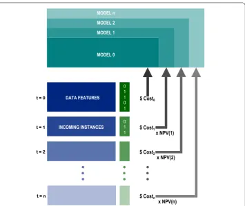
3.3 Predictions to dollar value
As shown in Figure , at every new batch of new incoming instances, predictions are made by all the classification strategies. Correctly classified values have an associated cost of , whereas false negatives and false positives come at different costs. In imbalanced datasets, where the positive class is deemed to be more important than the negative class, the cost of a false negative can be consideredηtimes greater than that of a false positive, where,
CFP= Cost of False Positives, andCFN= Cost of False Negatives.
CM=
CFP CFN
=
CFP ηCFP
=CFP
η
,
Figure 2 Predictions to dollar value: incoming instances are predicted upon and eachmisprediction costsa particular dollar amount.This dollar amount’s discounted value over time can be computed using its NPV. Each of these discounted values contribute towards modifying the underlying model for the next batch of incoming instances. This feedback mechanism strives to continuously improve the prediction model.
subject to differing cost objectives as trade-offs between false positives and false negatives. Conventionally, cost-sensitive learning is structured as follows:
. Get cost matrix (CM);
. Learn model (M) from training data (Tr) att= ;
. Learned model is optimized on cost matrix;
. Predict subsequent test data instances (Te) based on modelM;
. CombineTewith existing dataTr, and retrain modelMtoMto minimize costs;
. Repeat for subsequent instances.
Each batch generates an associated cost at that given time instance. Added to this cost, is the cost of whatever strategy is in effect — cost of external data, cost of model devel-opment, etc. This total cost needs to be contextualized in terms of its time value, and therefore an appropriate discount rate is applied and an NPV calculation is made over all the batches. Each strategy is evaluated in terms of NPV alone and compared with the baseline.
Thus, we suggest a modified approach:
. Get cost matrix (CM);
.-. . . .(same as before);
. CombineTewith existing dataTr;
. Retrain modelMtoMusing a discounted cost matrixCMand data costs;
The alteration here being thatCMis adiscountedcost matrix. This is in keeping with the time value of money, here costs. Costs in the future are relatively discounted versus those in the present. Mathematically, the difference between the two approaches may be stated as below:
CMconventional=CFP
η
,
CMproposed(r,t) =
CFP ( +r)t
η
,
where,r= discount rate, andt= time elapsed.
The reader may notice that a value of has been assigned to correctly predicting the class of any given test instance (i.e. the diagonal elements). This value is dependent on the business model, and in a pure form evaluation can be adjusted by the user.
Total Cost = n
t=
Misprediction + Ext. Data + Model Dev.
( +r)t .
This brings us to the overall comparison of the objective function: the cost. Our ap-proach is to calculate this cost function separately for each time value in the future. This makes it behave very different from the conventional static picture of cost sensitive learn-ing — e.g. an error in the immediate time frame is nowcostlierthan that same error oc-curring at a future time. More discussion on the Discount Rate is available in Additional file , Section .
3.4 Integrating with standard techniques
The total cost matrix derived in Section . can be directly integrated with contemporary cost-sensitive techniques, many of which are listed in ., thus enabling the generality of our work. The misprediction cost matrix for each time-wise batch can also be adjusted with the corresponding costs. If one ends up paying for external data and/or model devel-opment, then the modified misprediction cost matrix as shown below should account for all of our considerations so far:
CMmod(r,t) = ( +r)t
CFP η
+ (CExt+CModel)
.
The second matrix in the above equation considers costs for correctly classified in-stances as well. This is due to the fact that cost of external data acquisition and that of model development are agnostic of prediction outcome. Since this cost matrix is time sen-sitive, it is important that the correct version of this matrix be used for all considerations or else the NPV consideration would not be relevant to the desired time period. It should be noted that this modified cost matrix is consistent with the total cost calculations as per Section ..
3.5 Variable cost modeling
and false negatives may vary for each instance, e.g. in fraud detection for credit card trans-actions. Using the modifications suggested in [], we can transform the cost matrix into a function of the specific instance. The overall cost matrix for each batch now becomes a function of the averages of the variable costs:
CM=
CFP CFN
= i
icfp(i) icfn(i)
.
Upon considering the discounted NPV in Section . and various costs from Section ., we arrive at the following modified cost matrix:
CMmod(r,t) =
i ( +r)t
cfp(i)
cfn(i)
+cExt(i) +cModel
i .
Here, each instance has an associated cost of misprediction (cfpandcfn), a cost of external data acquisition, and a cost of model development. The cost of model development is assumed flat across all instances, socModelis the total cost of model development divided by the number of instances in the training data.
An aggregateηis still relevant in this case as an indication of relative costs. Micro and macro averaged versions of it may be used wherever relevant
ηmicro= i
cfn(i)
cfp(i)
i,
ηmacro=
i
cfn(i) i
cfp(i).
The above costs are known beforehand for the training set. In practice, one might not have this luxury for the test set. The paper by Zadrozny and Elkan [] obtains estimates of overall cost in the test set by establishing boundaries.
4 Experimental setup
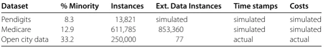
With the aim of demonstrating the above unification of concepts, we perform several ex-periments on the datasets listed in Table . We are not necessarily comparing methods, but rather demonstrating different use-case scenarios of the proposed NPVModel. To that end, the datasets represent data from popular and publicly available sources — the UCI Repository [], Medicare data [, ], and open city data [].
4.1 Datasets
UCI dataset - pendigits The imbalanced UCI Machine Learning Repository datasets are used in many standard cost sensitive learning papers in literature [, , ]. These are
Table 1 Datasets used: the aim is to get datasets which resemble those used in contemporary cost sensitive prediction tasksandhave corresponding external datasets
Dataset % Minority Instances Ext. Data Instances Time stamps Costs
standard datasets used in literature which have varying levels of binary class imbalance. Since this paper’s contribution is not directly tied to the number of instances in a dataset or its class imbalance, we choose the pendigits datasets as an example dataset from the UCI datasets. Choosing any other dataset would result in a similarprocessto glean insights and that is the overarching goal of this paper.
To establish baselines and preserve simplicity, the multiclass pendigits dataset has been converted to a binary class dataset in keeping with []. It should be noted that the tech-niques discussed in this paper can be directly extended to multiclass problems. Since the UCI datasets are meant for standalone prediction tasks, we discuss how external data in a dynamic form is simulated from UCI datasets in Additional file , Section .
Medicare data Medicare.gov contains official data from Centers for Medicare & Medi-caid Services (CMS). Given a set of descriptors, we would like to predict whether a given health care professional is a physician or not. The National Downloadable File contains information about all of the providers enrolled under the Medicare program []. This is to be considered our in-house data. The procedures they perform are enumerated in the Medicare Provider Utilization and Payment Data: Physician and Other Supplier file []. This file can be used as an external feature lookup dataset. The particulars of delineating class and feature selection are as per Section in Additional file .
The feature vector is composed of: location of medical school at a city level, graduation year from medical school, the gender of the health care professional and participation in various initiatives like PQRS [], EHR [], eRx [], Million Hearts []
Open city data The Public Safety dataset of crimes in Chicago can be used to predict whether an arrest will be made in a particular case. This dataset is available publicly [] and it reflects reported incidents of crime that occurred in the City of Chicago from to approximately the present day. As our external queryable feature-set, we have various census based socio-economic indicators at the “community area” level. With this in mind, we want to find the applicability of these socio-economic factors towards improving the predictive power of the crime reports dataset. The external data instances are queried using the relevant “community area”, thus postulating that socioeconomic factors may be indicative in predicting arrests.
4.2 Testing workflow
We take the datasets from Section . in batches (real or simulated, as the case may be). We then create external data queriedavatarsof them according to Section . and perform predictions as per Section . using techniques in Additional file , Section . We repeat this for various cost factors to cover different penalties for False Negatives.
5 Results
Figure 3 A heatmap of all strategies and their NPV costs for the pendigits dataset.Costs are represented in log10(·) form. A lower cost implies amore feasiblemodel. These are grouped according to
classification technique, how much external data has been acquired, and the rate of external data.
5.1 Interpreting the results
The key results here can be summarized in the form of a heatmap like the one in Figure containing external data strategies, classification techniques, amount of external data (if applicable), cost of external data. The heatmaps are shown with the respective baselines for the strategy: NPV costs for no external data purchased. The “warmer” the color is, the closer we are to the least cost NPV. Due to the varied nature of costs, the actual dollar amounts are expressed on a colormap in logarithmic scale. The optimal solution is the one which has the lowest NPV of costs. The broken line represents the feasibility boundary — all strategies which cost higher than this are infeasible. Case-wise constraints can be applied to this heatmap as per the specifications of the project e.g.: the cost of external data is fixed at a particular value, and/or only batched external data is available. In Figure , the best overall strategy is to get external data for free and use a cost sensitive decision tree. If the cost of external data is fixed at a certain amount, only the relevant column of this heatmap needs to be consulted. If the amount of external data instances is fixed at say . times the test instances, then only those rows are relevant to this analysis. A more in-depth analysis on price negotiation is available in Section ..
5.2 Should one get external data?
As the results in Figure indicate, it may not always be the best idea to get external data. In the pendigits dataset, it is directly advisable to acquire external data in the basic classifier model (DT). In order to consider the feasibility of a hybrid approach involving CSDT, one must also factor in the costs of model development as per specification. This is discussed in Section ..
Figure 4 Medicare data strategies and their NPV costs.For the medicare data, only the transactional external dataset is available, hence we only see Case D being used in the heatmap. This greatly benefits from upgrading to CSDT-dyn.
Figure 5 City data strategies and their NPV costs.This presents a strong case for using external data.
tree with a dynamic cost matrix decreases misprediction costs by almost two orders of magnitude than the baseline of no external data, naive model. Adding external data makes the prediction better for decision trees, but only up to a certain cost-per-instance of exter-nal data (between $ and $ in this case). For cost sensitive decision trees, adding exterexter-nal data turns out to be infeasible when compared to the respective in-house baseline.
In the Open City Data, Figure shows that model development pretty much halves the NPVs of costs. For very low cost external data, hybrid strategies involving both model development and external data are more feasible. We can see that adding external data priced below $. per instance is always beneficial for this dataset.
5.3 How much external instance data should one get?
Figure 6 How much external data?Depending on how much each instance effectively costs the business, we see two distinct regions of feasibility based on convexity of the curves. Certain costs for external data are omitted to aid clarity.
Figure 7 Model complexity for pendigits: the competing model here is a DT and the decision to upgrade the complexity to that of a CSDT relies on how much it costs to make the switch. In this case, as long as the cost is lower than the baseline (naive model, shown using the broken pink line), and below the competing model (shown using the starred black continuous line), it is feasible to use a CSDT.
$., the clear answer to the optimum amount of external instance data is % of the incoming instances.
5.4 Model development strategies
As seen in Figure , for a given external data strategy, model complexity costs can make a high performing sophisticated model (CSDT) infeasible against a competing simple model (DT). The margin between the competing simple model and the model under considera-tion can also be used to assign a maximum development budget. Model complexity can be addressed in the case of Figures and . In the Medicare data, CSDT-dyn helps bring down the costs of misprediction by far when compared to any other strategy for external data. For the Open City Data, CSDT-dyn helps bring down costs in terms of external data, but not the in-house model development baseline case.
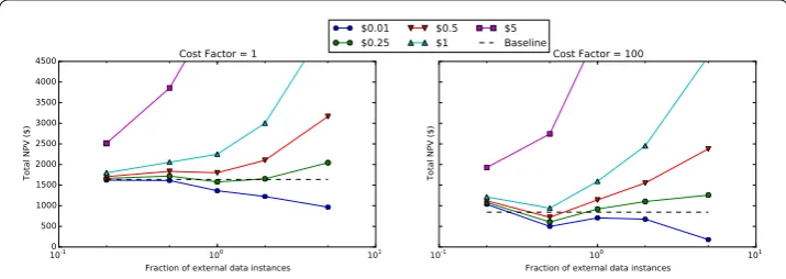
5.5 Cost factor
The heatmaps presented are generated for a given cost factor. For cost sensitive classifiers, changing the cost factor results in a change in the underlying trained models. The penalty for misclassified instances is fundamentally altered and hence this change may result in entirely different solutions emerging as “most feasible”. For the pendigits dataset, this can be seen with how NPVs for equivalent external data strategies get affected in Figure . Since both their baselines are different, we plot them on different charts and compare them side by side, keeping the axis limits the same.
Figure 8 Cost factor comparison: upon increasing the cost factor, cost sensitive models penalize false negatives more severely than false positives.This results in drastically different classifiers being trained for the same external data strategy.
and thus by sheer abundance, drives up the NPV costs. It is also evident that the convexity of the curves changes by changing the cost factor — the price-point of $ is a good exam-ple of this. The best strategy for a cost factor of is to get the same amount of external instances as the incoming instances. For a cost factor of , the best suggestion is to get half of the number of incoming instances instead.
In terms of strategy, inferences from one cost factor model arenotdirectly transferable to the other by simply adjusting for a different cost penalty model.
5.6 Price negotiation for external data
In order to minimize the total cost function, we would like to minimize the price for ex-ternal data. As seen from Figure , there exists a maximum permissible price-point, below which, acquiring external data is feasible. From a business perspective, it is thus useful to locate these points. It is to be noted that since these maximum permissible price-points are bound by feasibility, they are indirectly linked to the underlying cost factor. A higher cost factor would drive the maximum feasible price point higher, as can be seen from Fig-ure . For a cost factor of , it is feasible to acquire external data if each instance costs $. or less, whereas in the case of a cost factor of , we can afford to acquire external instances at $ each.
5.7 Scalability
NPVModel consists of two main components — () training models on data and () com-puting NPV over a search space of parameters. These parameters can include all relevant external data strategies (Section .), amount of external data (Section .), cost of exter-nal data (Section .), various candidate models (Section .), cost factor(s) (Section .) and discount factor(s) (Additional file , Section ).
The training component’s complexity is directly dependent on the classification tech-niques considered. NPVModel facilitates the use of any user-specified classifier to be con-sidered in the training stage, so the overall complexity for this stage is simply the complex-ity of the classifier. No additional cost is imposed by the NPVModel.
parameter cannot be changed, its cardinality in the grid search is simply equal to . All of the parameters listed in this paper appear as design choices in the complexity of imple-menting NPVModel.
For a given time, the cost computation is dependent on the respective model having been trained. Since the NPV calculation is independent across parameters, this becomes an embarrassingly parallel computation.
Overall, NPVModel’s scalability is directly affected by that of the training complexity of models considered (classifier dependent), the number of incoming test instances (linear), and of the parameter space one seeks to optimize over (multiplicative).
Throughout the experiments in the paper, we see that the insights can be derived for small datasets (pendigits) and for larger datasets (medicareandopen city data). The modified cost matrix defined in Section . is agnostic to the size of the dataset in question. This makes NPVModel a powerful and easy addition to the existing modeling techniques and considerations.
6 Conclusion
We proposed and demonstrated a unified framework, NPVModel, to help quantify the trade-offs between data acquisition and modeling. The main contribution of this paper is to serve as a strategy-board for business decisions when implementing and deploying analytics programs. Throughout the paper, effort has been made to address contemporary analytics and data science needs. In Section , we fill the gap in literature between external data acquisition, model development strategies, and provide a method to obtain a dollar value of predictive output. The methods outlined here can not only help choose a strategy for immediate use, but also provide a horizon for the future. Section discusses how an organization might need to think of cost factor and discount rate asdesign parametersin the context of their data science process. We not only demonstratewhetheror not it is a good idea to invest in external data or model development, but we also demonstrate which implementations of such strategies are worthwhile.
Future work In this paper, we considered the scenario that the acquisition of external feature data occurs for all instances in the dataset. That might not apply for all possi-ble use-cases. We propose that active learning can then be applied within this construct. Furthermore, we did not incorporate the notion of “data aging”, that is we place the same importance on older and newer data. So, it remains to be investigated whether older data’s value decays over time. If so, how does it affect data management strategies?
Additional material
Additional file 1: Quantifying decision making for data science: from data acquisition to modeling(pdf )
Competing interests
The authors declare that they have no competing interests.
Authors’ contributions
SN and NVC conceived of and designed the research. SN implemented the empirical analysis. SN and NVC wrote the paper. All authors read and approved the final manuscript.
Acknowledgements
Endnotes
a Modeling in our work assumes development and application of statistical or machine learning based
algorithms/methods and performing analytics.
b For example, one can compute at scale using Amazon Web Services’ (AWS) Elastic Compute Cloud (EC2) [25], which
“is a web service that provides resizable compute capacity in the cloud [25]” and is “designed to make web-scale cloud computing easier for developers [25]”.
Received: 27 January 2016 Accepted: 9 August 2016
References
1. Ling CX, Sheng VS (2010) Cost-sensitive learning. In: Encyclopedia of machine learning, pp 231-235
2. Lomax S, Vadera S (2013) A survey of cost-sensitive decision tree induction algorithms. ACM Comput Surv 45(2):16 3. Domingos P (1999) Metacost: a general method for making classifiers cost-sensitive. In: Proceedings of the fifth ACM
SIGKDD international conference on knowledge discovery and data mining. ACM, New York, pp 155-164 4. Witten IH, Frank E (2005) Data mining: practical machine learning tools and techniques
5. Chai X, Deng L, Yang Q, Ling CX (2004) Test-cost sensitive naive Bayes classification. In: Fourth IEEE international conference on data mining, 2004. ICDM’04. IEEE, New York, pp 51-58
6. Sheng VS, Ling CX (2006) Thresholding for making classifiers cost-sensitive. In: Proceedings of the national conference on artificial intelligence, vol 21. AAAI Press, Menlo Park, p 476.
7. Zadrozny B, Langford J, Abe N (2003) Cost-sensitive learning by cost-proportionate example weighting. In: Third IEEE international conference on data mining, 2003. ICDM 2003. IEEE, New York, pp 435-442
8. Ting KM (1998) Inducing cost-sensitive trees via instance weighting. Springer, Berlin
9. Domingos P (1998) How to get a free lunch: a simple cost model for machine learning applications. In: Proceedings of AAAI-98/ICML-98 workshop on the methodology of applying machine learning, pp 1-7
10. Weiss GM, Provost F (2003) Learning when training data are costly: the effect of class distribution on tree induction. J Artif Intell Res 19:315-354
11. Dalessandro B, Perlich C, Raeder T (2014) Bigger is better, but at what cost? Estimating the economic value of incremental data assets. Big Data 2(2):87-96
12. Weiss GM, Tian Y (2008) Maximizing classifier utility when there are data acquisition and modeling costs. Data Min Knowl Discov 17(2):253-282
13. Greiner R, Grove AJ, Roth D (2002) Learning cost-sensitive active classifiers. Artif Intell 139(2):137-174
14. Donmez P, Carbonell JG (2008) Proactive learning: cost-sensitive active learning with multiple imperfect oracles. In: Proceedings of the 17th ACM conference on information and knowledge management. ACM, New York, pp 619-628 15. TLOxp (2015) TLOxp Pricing alternatives available for all industries. http://www.tlo.com/pricing.html. [Online;
accessed 17-June-2016]
16. LexisNexis (2015) LexisNexis Pricing Plans. http://www.lexisnexis.com/gsa/76/plans.asp. [Online; accessed 02-June-2015]
17. Zadrozny B, Elkan C (2001) Learning and making decisions when costs and probabilities are both unknown. In: Proceedings of the seventh ACM SIGKDD international conference on knowledge discovery and data mining. ACM, New York, pp 204-213
18. Center for Medicare, Medicaid Service: Provider Utilization and Payment.
http://www.cms.gov/Research-Statistics-Data-and-Systems/Statistics-Trends-and-Reports/Medicare-Provider-Charge-Data/Physician-and-Other-Supplier.html. Accessed: 2015-03-16
19. Medicare Provider Utilization and Payment Data.
http://www.cms.gov/Research-Statistics-Data-and-Systems/Statistics-Trends-and-Reports/Medicare-Provider-Charge-Data/Physician-and-Other-Supplier.html. Accessed: 2015-06-03
20. Crimes 2001-present. https://data.cityofchicago.org/Public-Safety/Crimes-2001-to-present/ijzp-q8t2. Accessed: 2015-06-03
21. Physician Quality Reporting System.
http://www.cms.gov/Medicare/Quality-Initiatives-Patient-Assessment-Instruments/PQRS/. Accessed: 2015-06-03 22. The EHR Incentive Program.
http://www.cms.gov/Regulations-and-Guidance/Legislation/EHRIncentivePrograms/index.html?redirect=/ EHRIncentiveprograms. Accessed: 2015-06-03
23. The ERx Incentive Program.
https://www.cms.gov/Medicare/Quality-Initiatives-Patient-Assessment-Instruments/ERxIncentive/index.html? redirect=/ERxIncentive/. Accessed: 2015-06-03