Graph clustering‑based discretization
of splitting and merging methods (GraphS
and GraphM)
Kittakorn Sriwanna
*, Tossapon Boongoen and Natthakan Iam‑On
Background
Discretization is a data reduction preprocessing technique in data mining. It transforms a numeric or continuous attribute to a nominal or categorical attribute by replacing the raw values of a continuous attribute with non-overlapping interval labels (e.g., 0–5, 6–10, etc.). Different data mining algorithms are designed to handle different data types. Some are designed to handle only either numerical data or nominal data, while some can cope with both. Because real datasets are always a combination of numeric and nominal vales, for an algorithm that only takes nominal data, numerical attributes need to be dis-cretized into nominal attributes before the learning algorithm. After discretization, the subsequence mining process may be more efficient as the data is reduced and simplified resulting in more noticeable patterns [1–3]. Moreover, discretization is also expected to improve the predictive accuracy for classification [4] and Label Ranking [5].
Abstract
Discretization plays a major role as a data preprocessing technique used in machine learning and data mining. Recent studies have focused on multivariate discretiza‑ tion that considers relations among attributes. The general goal of this method is to obtain the discrete data, which preserves most of the semantics exhibited by original continuous data. However, many techniques generate the final discrete data that may be less useful with natural groups of data not being maintained. This paper presents a novel graph clustering‑based discretization algorithm that encodes different similarity measures into a graph representation of the examined data. The intuition allows more refined data‑wise relations to be obtained and used with the effective graph cluster‑ ing technique based on normalized association to discover nature graphs accurately. The goodness of this approach is empirically demonstrated over 30 standard datasets and 20 imbalanced datasets, compared with 11 well‑known discretization algorithms using 4 classifiers. The results suggest the new approach is able to preserve the natural groups and usually achieve the efficiency in terms of classifier performance, and the desired number of intervals than the comparative methods.
Keywords: Multivariate discretization, Graph clustering, Normalized cuts, Normalized association, Data mining
Open Access
© The Author(s) 2017. This article is distributed under the terms of the Creative Commons Attribution 4.0 International License (http://creativecommons.org/licenses/by/4.0/), which permits unrestricted use, distribution, and reproduction in any medium, provided you give appropriate credit to the original author(s) and the source, provide a link to the Creative Commons license, and indicate if changes were made.
RESEARCH
Two main goals of discretization are to find the best intervals or the best cut points1 and to find the finite number of intervals or the number of cut points that are better adapted to the learning. Therefore, modelling a discretization requires the development of the following two subjects. First, discretization criterion is the criterion made for choosing the best cut points in order to split a set of distinct numeric value into intervals (Splitting, Top–Down methods) or merge a pair of adjacent intervals (Merging, Bot-tom–Up methods). Second, stopping criterion is a criterion for stopping the discretiza-tion process in order to yield the finite number of intervals.
The process of discretization typically consists of 3 main steps that are sorting attrib-ute values, finding the cut-point model or discretization scheme of the attribattrib-utes by iter-ative splitting or merging, and finally, assigning each value in the attribute with a discrete label corresponding to the interval it falls into. Hence, the number of intervals obtained for attributes under question may be different depending on the number of possible cut points, the relation with the target class, for instance.
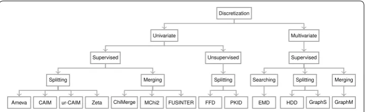
Discretization techniques can be classified in several different ways, such as supervised versus unsupervised, univariate versus multivariate, splitting versus merging, direct ver-sus incremental, and more [6–9]. Supervised methods consider the class information, whereas unsupervised ones do not consider the class information. Splitting algorithms start from one interval and recursively select the best cut point to split the instances into two intervals, while merging methods begin with the set of single value intervals and iteratively merge adjacent intervals. The univariate category discretizes each attribute independently without considering its relationship between other attributes. However, multivariate methods also consider other attributes to determine the best cut points. Direct techniques require inputting the number of intervals supplied by the user. Exam-ple of this type of methods are equal-width and equal-frequency discretization algo-rithms [10]. The number of intervals is equal for all attributes in these algorithms. In contrast, incremental methods do not require the number of intervals, but they require the stopping criterion to stop the discretization process in order to yield the best num-ber of intervals of each attribute.
Most discretization algorithms proposed in the past were univariate methods [3]. Chi-Merge [11], Chi2 [12], Modified Chi2 [13], and area-based [14] are examples of univari-ate, supervised, incremental and merging methods. They use statistic-based algorithms to determine the similarity of adjacent intervals. They divide the instances into intervals and then merge adjacent intervals based on χ2 distribution. CAIM [15], ur-CAIM [16], and CADD [17] are univariate, supervised, incremental and splitting methods. These algorithms use class-attribute interdependence information as the discretization crite-rion for the optimal discretization with a greedy approach, by finding locally maximum values of the criterion. Ent-MDLP [18], D-2 [19], and FEBFP [20], which are univariate, supervised, incremental and splitting methods, recursively select the best cut points to partition the instances based on the class information entropy [10]. PKID and FFD [21] are univariate and unsupervised methods that maintain discretization bias and variance by tuning the interval frequency and the interval numbers, especially used with Naive-Bayes classifier.
The fact that univariate methods discretize only a single attribute at a time and do not consider interactions among attribute, may lead to important information loss [3] and not getting a global optimal result [22]. ICA [22], Cluster-Ent-MDLP [23], HDD [3], and Cluster-RS-Disc [24] are examples of multivariate discretization methods. ICA, tries to get a global optimal result by transforming the original attributes to new attribute space that considers other attributes. Then, it discretizes the new attribute space using the uni-variate discretization method (Ent-MDLP). Cluster-Ent-MDLP, similar to ICA, finds the pseudo-class by clustering the original data via k-means [25] and SNN [26] clustering algorithms and then uses the target class and pseudo-class to discretize using the uni-variate discretization method (Ent-MDLP). It finds the best cut point by averaging both entropies that considers the target class and pseudo-class. HDD extends the univari-ate discretization method (CAIM) by improving the stopping criterion and taking into account information specific to other attributes. Cluster-RS-Disc attempts to obtain the natural intervals of attribute values by first partitioning using DBSCAN [27] clustering algorithm. After that, it discretizes an attribute based on the rough set theory.
Although several multivariate discretization algorithms overcome the drawback of univariate discretization methods by considering interactions among attributes, there are some weaknesses. Some of them have made use of cluster labels as a part of dis-cretization criterion. As a matter of fact, different clustering algorithms or even the same algorithm with multiple trials may produce different cluster labels. Therefore, it is extremely difficult for a user to decide the proper algorithm and parameters [28–30]. Despite the reported improvement, some multivariate discretization algorithms such as EMD [31] do not concentrate the natural group of data. In fact, EMD is an evolutionary discretization algorithm that defines the fitness function based only on high predictive accuracy and lower number of intervals. Hence, the identified cut points may damage the natural group of data.
In order to solve the aforementioned problems, this study presents a novel graph clustering based algorithm that allows encoding of different similarity measures into a graph representation of the examined data. Instead of using cluster labels, the pro-posed method uses the similarity between data pair, which is the weighted combination between distance and target-class agreement. Each pair of data is formed into graph, which is then partitioned in order to find the appropriate set of cut-points. The insight-ful observations and the benefit of graph clustering are present as follows.
The main graph clustering formulations are based on graph cut and partitioning problems [39, 40]. According to the research of Foggia et al. [36], the performance of five graph clustering algorithms: fuzzy c-means MST (minimum spanning tree) clus-tering [41], Markov clustering [34, 42], iterative conductance cutting algorithm [43], geometric MST clustering [44], and normalized cut clustering [40] are evaluated and compared. Based on this empirical study, it is confirmed that the normalized cut cluster-ing provides good performance and appears to be robust across application domains. The normalized cut criterion avoids any unnatural bias for partitioning out small sets of points [40]. It is used in many works such as image segmentation and spectral cluster-ing [45, 46].
With these insightful observations, the paper introduces new discretization algo-rithms, which exploit graph clustering and the normalized cut criterion. Because the minimum normalized cut criterion is equivalent to the maximum normalized associa-tion criterion (see “Measures with clusters” for details), to design the stopping criterion, this normalize association criterion is chosen in this study. In particular, two new graph clustering-based techniques, which are splitting method (GraphS) and merging method (GraphM), are proposed. It is worthwhile to highlight several aspects of the proposed models here:
• The proposed discretization algorithms are incremental and multivariate methods. They find the number of cut points automatically and preserve the natural group of data by considering the correlation dependence among the attributes.
• The algorithm encodes information of data under examination as a graph, where the weight of each edge is evaluated by both natural distance and class similarity. This is a novel with the capability to address both data-wise relation and class-specific in the same decision making process.
• The normalize cut criterion prevents an unnatural bias that partitions out a small set of points. It helps to avoid acquiring too-small-size intervals with only a few mem-bers, thus demoting the over-fit problem.
The rest of this paper is organized as follows. “Graph clustering and partitioning prob-lems” provides the basis of graph clustering as to set the scene for proposed work and following discussions. In “A novel graph clustering-based approach”, the new algorithms are presented with related design issues being explained. The performance evaluation is included in “Performance evaluation”, based on the experiments with a rich collection of benchmark data. The paper is concluded in “Conclusion”, with possible future work.
Graph clustering and partitioning problems
In this paper, the undirected weighted graph with no self-loops and global graph cluster-ing are focused. Global graph clustercluster-ing assigns all of the vertices to a cluster, whereas local graph clustering only assigns a certain subset of vertices [35]. In brief, the reviews in this section are on these two types of undirected weighed and global graph clustering.
where ω(u,v) is the positive weighting of the edges. Let the set of partitioning or
cluster-ing of G be πk = {C1,. . .,Ck}, where Ci is a cluster in k sub-clusters.
Clustering measures
Measure with vertices
This type of measures is based on similarities or distances of the object pairs. They are used to apply to many areas such as pattern recognition, information retrieval, and clus-tering [47]. The common distance measures that are used in clustering are Euclidean and Manhattan distance [48].
Euclidean distance It simply is a geometric distance in a multidimensional space. It is a multivariate extension of the Pythagorean distance between two points. The formula for this distance between data points u(u1,. . .,ud) and v(v1,. . .,vd.) with d dimensions is shown in the Eq. 1.
Manhattan distance It is also called the City-block distance, Rectilinear distance, and Taxicab norm. The result of this distance is the distance similar to Euclidean distance. However, the effect of outliers is dampened because they are not taking the square root [49]. The distance is computed as the Eq. 2.
Measures with clusters
Graph clustering is dividing a graph into groups (cluster, subgraph) that vertices highly connect in the same group [50]. To compare the quality of a given cluster C, the cluster fitness measure (quality function) or indices for graph clustering [33, 44, 51] are used [35,
52]. This study categorizes the clustering indices into two groups: density measures, and cut-based measures.
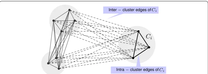
Density measures In the wrok of Görke et al. [53], many density measures such as intracluster density, intercluster density, intercluster conductance, and modularity are examined. These measures are used for unweighed graphs. They compute with number of vertices and edges in a cluster and another clusters. Brandes et al. [44] proposed the coverage of the graph clustering based on the number of intra-cluster edges and inter-cluster edges as shown in Eq. 3, where m(Ci,Ci) and m(Ci,C¯i) are the numbers of intra-edges and inter-intra-edges in the cluster Ci respectively. Those edges are shown in Fig. 1. A large value of coverage indicates the better quality.
Cut-based measures In undirected weighted graphs, graph-cut techniques such as ratio cut [54], min–max cut [55], and normalized cut [40] are mostly used to solve graph
(1)
distE(u,v)=
d
i=1
(ui−vi)2
(2)
distM(u,v)= d
i=1
|ui−vi|
(3)
coverage(Ci)=
partitioning problem, which are ones of the main keys to graph clustering algorithms. Those measures are formulated in Eqs. 4, 5, and 6 respectively, where ω(Ci,Ci) and ω(Ci,Ci¯) are the sum of weighted edges of inter-cluster edges and intra-cluster edges of Ci, respectively; n(Ci) is the number of vertices in the cluster Ci.
The smallest value of these criteria indicates a better quality of partitioning. Normalized cut avoids unnaturally partitioning out any too small set of vertices by taking the frac-tion out of the total weighted edges connected to all nodes in the graph. On the other hand, instead of considering the minimum cut among the clusters, partitioning can be done based on the maximum connection, called normalized association, as defined in Eq. 7. In addition, normalized association can define as Eq. 8.
provided that
(4) Ratio Cut(πk)=
k
i=1
ω(Ci,C¯i)
n(Ci)
(5)
Min Max Cut(πk)=
k
i=1
ω(Ci,C¯i)
ω(Ci,Ci)
(6)
NCut(πk)= k
i=1
ω(Ci,C¯i)
ω(Ci,Ci)+ω(Ci,C¯i)
(7)
NAsso(πk)=
k
i=1
ω(Ci,Ci)
ω(Ci,Ci)+ω(Ci,C¯i)
(8) NAsso(πk)=NAsso(C1)+NAsso(C2)+ · · · +NAsso(Ck)
(9)
NAsso(Ci)=
ω(Ci,Ci)
ω(Ci,Ci)+ω(Ci,Ci¯)
Ci
Ci
C
iThe minimum NCut and the maximum NAsso are equivalent and naturally related as NAsso(πk)=k−NCut(πk). In the authors’ observation, the coverage(Ci) is similar to NAsso(Ci), which changes the number of edges to the sum of weighted edges as demon-strated in [33].
Global graph clustering
The problem of global graph clustering is a dividing or grouping each vertex in the graph into clusters of predefined size, such that vertices in the same cluster are highly related and less related with vertices in the other clusters. The main clustering problem is NP-hard; therefore, the algorithms selected are approximation algorithm, heuristic algo-rithm, or greedy algorithm [35] so that the computation time is reduced.
Spectral clustering
The main tool for spectral clustering is the Laplacian matrices technique [56]. The algo-rithm transforms the affinity matrix (similarity matrix) into Laplacian matrix of the graph and then finds the eigenvector and eigenvalue from the matrix. Each row of eigen-vector represents a vertex (data point). The final stage is clustering or partitioning of those vertices by recursive two-way (bipartition) or direct k-way [39].
The unnormalized k-means algorithm [57] is an example of direct k-way clustering. It clusters the vertices using k-mean algorithm with the number of desired clusters. The two-way normalized spectral clustering (2NSC) and k-way normalized spectral cluster-ing (KNSC) algorithms are proposed by [40] to solve the generalized eigenvalue system using NCut criterion. 2NSC is a recusive two-way clustering that the number of clusters is controlled directly by the maximum allowed NCut value, whereas KNSC is direct k-way clustering based on k-mean algorithm.
Markov chains and random walks
The Markov cluster algorithm (MCL) [34] finds the cluster structure in the form of graphs using the mathematical bootstrapping procedure. The main idea of MCL is to simulate the flow within a graph, promote the flow where the current is strong and demote the flow where the current is weak. If there is any natural group in the graph, the current across between groups will wither away. The algorithm also simulates random walks within a graph, starting from a vertex and randomly travelling to another vertex that connected with many steps. Travelling within the same cluster is more likely than across the other cluster.
A novel graph clustering‑based approach
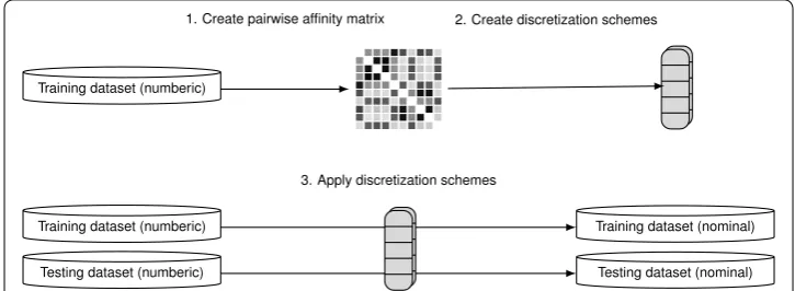
This section introduces a new graph clustering-based approach to discretization problems. Figure 2 summarizes the entire process of the proposed framework, which includes three main steps: (1) create the affinity matrix using the pairwise distances and class similarity, (2) create discretization schemes, and (3) discretize the datasets by applying the discretization schemes.
representation of this dataset is demonstrated in Fig. 3b. It assigns the weight of each edge between each pair of the data points based on similarity, which both target class and distance are considered. If the data points of the pair are close and in the same class, the edge will have a high score. This scoring is stored in the affinity matrix (see “Pairwise affinity matrix” for details). After that, graph clustering is used to find the best cut point that cuts the minimum weighted edge as shown in Fig. 3c, where vertical and horizontal dashed lines are the best cut points that cut minimum weighted edges of attributes A1
and A2, respectively (see “Graph clustering-based discretization algorithm” for details).
Fig. 2 Proposed framework. The framework of the graph clustering‑based discretization. A graph clustering‑ based algorithm first creates the affinity matrix to represent a graph; then, generates a discretization scheme of each numeric attribute. Finally, the numeric attributes are transformed into the nominal attributes by applying the dicretization schemes
a
b
c
Fig. 3 Graph representation of data points. Example of a the scatter plot of the toy dataset, b the proposed
graph representation of data points, and c the cut point selections that cut the minimum weighted edges.
Pairwise affinity matrix
The pairwise affinity matrix (AF matrix) is an n×n matrix that contains the similarity scores of the pair of data points, where a high score means the pair has high similarity. In this study, the graph is represented by an AF matrix. The distance and class similar-ity values of the pair are considered for scoring in order to find the similarsimilar-ity. Before scoring, each value of the data points xi in the numeric attribute Aj, valij is the rescaled (normalized) between 0 and 1 in order to give all attributes the same treatment as shown in Eq. 10, where val∗
ij is new rescale value of valij, minAj and maxAj are the minimum and maximum values of the attribute Aj, respectively.
In this study, the similarity measure, sim(u, v), is proposed as Eq. 11. It contains 2 main measures. First, simC(u, v) is a class-label measure of a pair of the data points u and v. Second, the distance measure, based on the Euclidean distance (see Eq. 1), adds a frac-tion of the number of attribute d in the square root in order to normalize the distance to be between 0 and 1 and subtracts the distances from 1 in order to change to the similar-ity (small distance values indicates high similarsimilar-ity). In addition, the distance of a pair in the nominal attribute is set to 1 if the pair has the same value and 0 otherwise.
provided that
The proposed similarity measure considers both the distance and class labels for scoring. The measure weights those values equally by combining them altogether. Each element in the AF matrix contains the sim(u, v) value of each data-point pair, and AF∈ [0, 2]n×n.
Graph clustering‑based discretization algorithm
Typically, the discretization algorithm discretizes attribute one by one. The process con-sists of three main processes. First, sorting an attribute Ai and finding all the possible cut points. Second, finding the cut point model of the attribute by iteratively finding the model one by one until discretization is complete on all of the numeric attribute. Finally, transforming the numeric attribute to the nominal attribute.
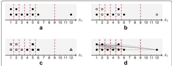
In order to show the difference of the data view of the proposed algorithm, an example of the Toy dataset shown in Fig. 3 is again considered. The dataset has 2 numeric attrib-utes, A1 and A2. In order to discretize the attribute A1, the data views of discretization
algorithms are different depending on discretization methods. Figure 4 shows the four different data points views.
(10)
valij∗= valij− minA
j maxAj−minAj
(11)
sim(u,v)=simC(u,v)+
1− �
�d
i=1(ui−vi)2 d
,
(12)
simC(u,v)=
• After sorting the attribute A1, discretization algorithm that is unsupervised and
uni-variate method only considers the cut points as shown in Fig. 4a. The algorithm selects the cut point that all intervals have the similar number of data points or similar length.
• For discretization algorithm that is the supervised and univariate method, after sort-ing A1, the algorithm only considers the class labels as shown in Fig. 4b. The
algo-rithm discretized based on the purity class. The data points with the same class label are grouped. However, this method does not consider other attributes; therefore, it tends to lose the natural group.
• The Cluster-Ent-MDLP [23] is an example of supervised and multivariate method. This type of algorithms includes other attributes into consideration. The data are clustered and labelled. Then, the algorithm discretizes by considering class labels (see Fig. 4b for details) and cluster labels (see Fig. 4c for details) together.
• In the proposed algorithm, the data point view is based on the graph as shown in Fig. 4d. The vertices represent the data points and the edges’s weights represent the scores of sim-ilarity of the vertex pairs (see “Pairwise affinity matrix”). As both class and cluster labels are considered, this data view preserves much more information than the other views.
As the benefit of the data view under graph representation, this paper proposed 2 dis-cretization algorithms using this data view: spiting and merging methods. The discre-tization criterion and stopping criterion of these algorithms are based on the NAsso criterion (see “Measures with clusters” for details). The algorithms attempt to find the best set of cut points so that the data points in each cluster after partitioning are mostly similar judging from the weighed edges.
The proposed splitting discretization algorithm
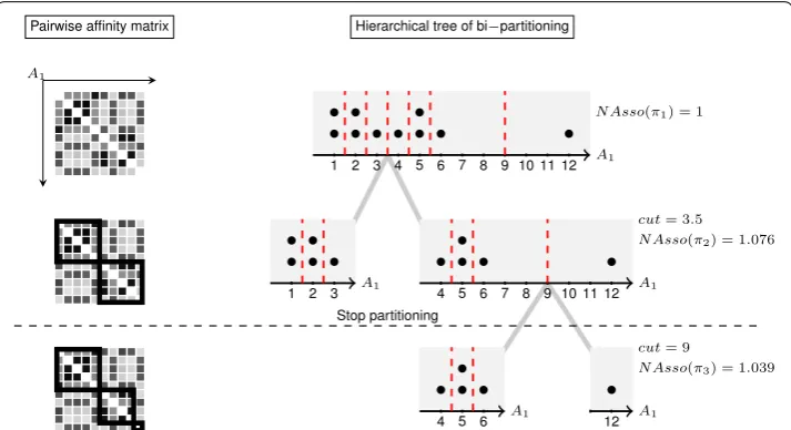
In the basis of splitting methods (top–down methods), all data points are grouped into clus-ters/intervals. The algorithms add a new cut point to bi-partition the clusters iteratively. The process stops partition until the number of cut points is satisfied. Similarly, the proposed splitting discretization bi-partitions the clusters as a tree structure as shown in Fig. 5.
a
b
c
d
In this proposed top–down algorithm, the discretization criterion of NAsso is used to consider the best new cut point. This criterion based on the sum of weights of intra-cluster and inter-intra-cluster. To easily find these values, the order of the pairwise affinity matrix is used to calculate. Figure 5 is an example of discretization of attribute A1 of the
Toy dataset. The procedures are as follows:
• Firstly, reorder the pairwise affinity matrix of A1 in ascending as shown in the top
matrix in Fig. 5. The matrix is 10×10 elements. Each element contains the
pair-sim-ilarity value, which in this example is represented by color, where a dark color indi-cates high similarity and a light color indiindi-cates low similarity.
• Then, calculate the NAsso values of all possible cut points (vertical dashed-lines). The example of calculating NAsso value of the cut point 3.5 is shown in the middle pair-wise affinity matrix. The two square boxes in the matrix are the intra-cluster weights of 2 partitions. The row outside the box is the inter-cluster weight of the boxed. The algorithm calculates NAsso values of all 6 cut points and select a cut point at 3.5 according to its highest NAsso values. Then, it bi-partitions a graph into 2 clusters.
• Finally, iteratively find the new best cut point until the stopping criterion is satisfied. In the figure, the second cut point is 9 with the highest NAsso value of 1.039. Because the value does not improve the NAsso value at the previous cut point (cut=3.5,
NAsso=1.076), the stopping criterion is stratified and stops at the previous step (see
next paragraph for the details). Hence, attribute A1 has 2 intervals with the cut point
at 3.5.
The proposed stopping criterion is based on the significant improvement of NAsso val-ues, as the higher NAsso denotes the higher similarity or community of data points in each cluster. If NAssso value drops or does not significantly improve after partitioning, it should stop discretization. The proposed stopping criterion is shown in Eq. 13, where NAsso(πi) and NAsso(πi−1) are NAsso values of the graph partitioning results with the
set of i and i−1 clusters, respectively, and β is the significant improvement percent-age. If the stopping criterion is true, the discretizaton will stop and the result is given as
π∗=πi−1.
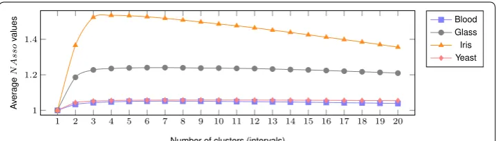
The examples of the trend of NAsso value (average of all numeric attributes) of 4 real datasets obtained from the benchmark UCI repository [58] of blood, glass, iris, and yeast are illustrated in Fig. 6. It shows that, for all 4 datasets, when increasing the num-ber of clusters (numnum-ber of intervals), the NAsso values drastically increase at the begin-ning, then slowly increase and finally slowly decrease. To prevent over partitioning at the slowly increasing of NAsso value, the new NAsso value, NAsso(πi), should be signifi-cantly better than the previous NAsso value, NAsso(πi−1). This study sets the new NAsso value should have 1% higher in significance than the previous value i.e., β=1.01 (see “Parameter analysis” for details).
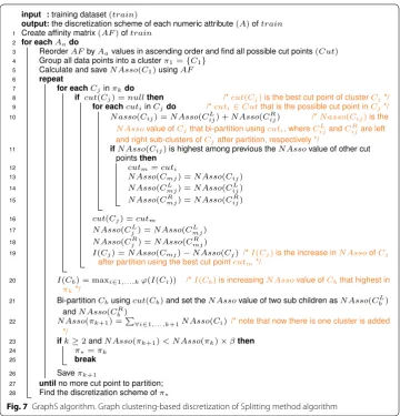
The details of the proposed splitting graph clustering-based discretization algorithm is shown in Fig. 7.
The proposed merging discretization algorithm
In contrast to splitting methods, the basic merging methods (bottom–up methods) start from many initial clusters. Each initial cluster contains data points that have the same attribute value. The algorithm iteratively merges the adjacent pair of clusters that the data points of the pair are most similar until the stopping criterion is met.
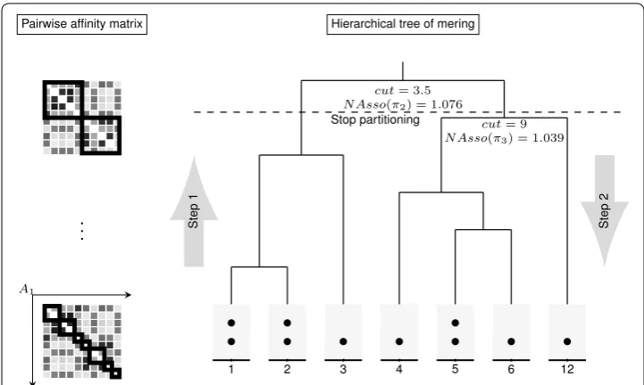
The proposed merging discretization algorithm includes 2 main steps. The first step is creating initial clusters, the data points in the clusters have the same attribute value. After that, the adjacent initial clusters that are given highest NAsso value after merging are selected to merge. The algorithm iterates merging the adjacent clusters, one by one until all of the clusters is grouped into a single cluster (1 interval), its forming is like a hierarchical tree as shown in Fig. 8. The next step is finding the best set of clusters (π∗) by examining top-down. This step starts from two intervals. It selects three intervals or higher intervals if significantly improve the NAsso value.
For demonstrating an example of this process, the Toy dataset is used again as shown in Fig. 8. In the first step, the initial clusters are created by grouping the data points of attribute A1 that have the same attribute values and reordered the values in ascend-ing. The initial clusters have 7 clusters, π7= {C1,C2,. . .,C7}. After that, two adjacent
(13) NAsso(πi) <NAsso(πi−1)×β
clusters that have highest NAsso values are merged until all clusters are grouped into one cluster (π1). In Fig. 8, the adjacent clusters of the cut point at 1.5, two initial clusters
that contain attribute values of 1 and 2 possess the highest NAsso value, therefore, this pair is merged first. The adjacent clusters (intervals) are merged further until only one cluster whose NAsso value is 1 remained. In the second step, the best set of clusters (π∗) is searched by evaluating the NAsso values top–down. This bottom–up algorithm uses the stopping criterion as in the top–down algorithm (see Eq. 13). As one can see that, the set of 3 clusters (π3) separated by the cut point of 9, the NAsso(π3) value is 1.039 that less than 1.076 of the NAsso(π2) value in the set of 2 clusters, hence π∗=π2.
The detail of the proposed merging graph clustering-based discretization algorithm is shown in Fig. 9.
Numeric to nominal transformation
In Fig. 7 (GraphS algorithm) and Fig. 9 (GraphM algorithm), each cluster in π∗ is equal to the interval, which contains the data point values. The intervals are transformed to discretization scheme as Eq. 14, where DA is a discretization scheme of attribute A, and cuti is the result of cut point selection of attribute A.
In the example of attribute A1 of the Toy dataset, the cut point list has only 1 cut point at
3.5. The discretization scheme of the attribute is {(−∞, 3.5],(3.5,+∞]}. In this study, the numeric values of A1 that are equal or less than 3.5 would be changed to “(inf_3.5]” and (14)
DA= {(−∞,cut1],(cut1,cut2],. . .,(cutk,+∞)}
Fig. 8 GraphM. The affinity matrix and hierarchical tree views of the proposed merging discretization algo‑ rithm
the values that are higher than 3.5 are denoted as “(3.5_inf]”. Each value of the numeric attribute is transformed to the interval name by checking the condition in the discretiza-tion scheme.
Performance evaluation
This section presents the performance evaluation of the graph clustering-based approaches that are splitting approach (GraphS) and merging approach (GraphM). In order to show the goodness of the proposed approaches that can handle with real world applications, this study investigated 30 real standard datasets and 20 imbalanced data-sets. This study evaluates the proposed methods by comparing with 11 discretization algorithms using 4 classifiers with the objective to evaluate and compare the perfor-mance of the selected discretization algorithms.
Investigated datasets
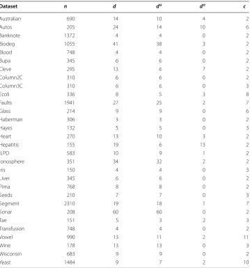
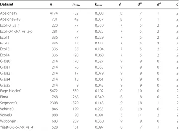
The experimental evaluation is conducted on 30 standard datasets and 20 imbalanced datasets. The standard datasets obtained from the benchmark UCI repository [58] as summarized in Table 1. The imbalanced datasets achieved from Keel-dataset reposi-tory [59, 60] as described in Table 2. In these datasets, some datasets have only numeric attributes and some have both numeric and nominal attributes. Because a small number of distinct values of a numeric attribute could be ambiguous with the nominal attribute. In the table, a numeric attribute with no more than two distinct values is regarded as a nominal attribute. This study also evaluated the Toy dataset (see Fig. 3 for details) in order to compare the different results of the algorithms of interest.
Experiment design
An experiment is set up to investigate the performance of the proposed algorithms com-pared to 11 discretization algorithms, which have variously different techniques. For comparison, 4 classifiers of: C4.5 (j48) [61], K-Nearest Neighbors (KNN) [62], Naive Bayes (NB) [63], and Support Vector Machine (SVM) [64] classifiers which are in the top 10 algorithm in data mining [65, 66] are examined.
The standard datasets considered are partitioned using the tenfold cross-validation procedure [67]. Each discretization algorithm performed with pairs of 10 training and 10 testing of each dataset. For the imbalanced datasets, each dataset was separated in five-fold already, this study evaluates them using fivefive-fold cross-validation procedure.
The performance measures
To evaluate the quality of the discretization algorithms, the following 3 measures are employed: number of intervals, running time, and predictive accuracy, respectively.
The number of intervals The result of the number of intervals is expected to be a small number as a large number of intervals may cause the learning to be slow and ineffec-tive [7, 19], and the small number of intervals is easier to understand. However, too sim-ple, too small discretization schemes may lead to lose classification performance [16].
Furthermore, this study compared the average number of intervals per attribute of the discreteization algorithms. Let Du= {d1u,d2u,. . .} be a set of numeric attributes,
intervals per attribute of dataset rx, AI(rx) is computed as Eq. 15, where NC(diu,rx)+1 is the number of intervals of attribute diu in the dataset rx.
The running times To create a discretization scheme (cut points model), the process of discretization is done only once with the training dataset. It seems to be an important evaluation; however, it should not take too long in order to be able to discretize with the real world dataset, which normally high number of data points.
The predictive accuracy The successful discretization algorithm should perform discre-tization such that the predictive accuracies are increased or without significant reduc-tion of predictive accuracy. This study evaluates the classificareduc-tion performance of 30
(15)
AI(rx)=
1
|Du| |Du|
i=1
NC(diu,rx)+1
Table 1 Description of 30 standard datasets
n, number of instances; d, number of attributes; du, number of numeric attributes; do, number of nominal attributes; c,
number of classes
Dataset n d du do c
Australian 690 14 10 4 2
Autos 205 24 14 10 6
Banknote 1372 4 4 0 2
Biodeg 1055 41 38 3 2
Blood 748 4 4 0 2
Bupa 345 6 6 0 2
Cleve 295 13 6 7 2
Column2C 310 6 6 0 2
Column3C 310 6 6 0 3
Ecoli 336 8 5 3 8
Faults 1941 27 25 2 7
Glass 214 9 9 0 6
Haberman 306 3 3 0 2
Hayes 132 5 5 0 3
Heart 270 13 10 3 2
Hepatitis 155 19 6 13 2
ILPD 583 10 9 1 2
Ionosphere 351 34 32 2 2
Iris 150 4 4 0 3
Liver 345 6 6 0 2
Pima 768 8 8 0 2
Seeds 210 7 7 0 3
Segment 2310 19 18 1 7
Sonar 208 60 60 0 2
Tae 151 5 3 2 3
Transfusion 748 4 4 0 2
Vowel 990 13 11 2 11
Wine 178 13 13 0 3
Wisconsin 683 9 9 0 2
standard datasets using predictive accuracy. The predictive accuracy results of the data-set are summarized by the mean of its 10 folds.
AUC Because the predictive accuracy is not a suitable measure for imbalanced data, this study evaluates 20 imbalanced datasets using AUC (area under the ROC curve) [68,
69]. The AUC is wildly used for classification evaluation for imbalanced data [70, 71], which measure the diagnostic accuracy of a test. The AUC value lies between 0 and 1, the higher value is the better average accuracy test. This study summarized AUC results of 20 imbalanced dataset by the mean of its 5 folds.
Statistical analysis
In this study, the ranking of discretization algorithms is obtained from the Friedman test [72, 73]. The discretization algorithm that obtains the lowest rank value is the better performance. Friedman test is non-parametric statistical test for assessing the difference between several related samples. It gives the mean rank for each discretization algorithm based on median difference, such that the algorithm with high averaged accuracy may not be in the first rank. If the Friedman test can show that at least one algorithm is signif-icantly different from at least another algorithm (using a level of significance α=0.05 ),
two post-hoc tests of Nemenyi and Holm are used to find the significantly different.
1. The Nemenyi post-hoc test [74] is used to find the critical difference (CD). Two algo-rithms are significantly different if the corresponding average ranks differ by at least the CD (using 95% confident level).
Table 2 Description of 20 imbalanced datasets
n, number of instances; nmin, number of minority classes; kmin minority class ratio; d number of attributes; du, number of numeric attributes; do, number of nominal attributes; c, number of classes
Dataset n nmin kmin d du do c
Abalone19 4174 32 0.008 8 7 1 2
Abalone9‑18 731 42 0.057 8 7 1 2
Ecoli‑0_vs_1 220 77 0.350 7 5 2 2
Ecoli‑0‑1‑3‑7_vs_2‑6 281 7 0.025 7 5 2 2
Ecoli1 336 77 0.229 7 5 2 2
Ecoli2 336 52 0.155 7 5 2 2
Ecoli3 336 35 0.104 7 5 2 2
Ecoli4 336 20 0.060 7 5 2 2
Glass0 214 70 0.327 9 9 0 2
Glass1 214 76 0.355 9 9 0 2
Glass2 214 17 0.079 9 9 0 2
Glass4 214 13 0.061 9 9 0 2
Glass5 214 9 0.042 9 9 0 2
Page‑blocks0 5472 559 0.102 10 10 0 2
Pima 768 268 0.349 8 8 0 2
Segment0 2308 329 0.143 19 18 1 2
Vehicle0 846 199 0.235 18 18 0 2
Vowel0 988 90 0.091 13 11 2 2
Wisconsin 683 239 0.350 9 9 0 2
2. The Holm post-hoc test [75, 76] is used to find the p-value of the post-hoc Holm (pHolm) of each pair comparison. The discretization algorithm that obtains the lowest
rank value is set as a control algorithm. The control algorithm is compared against the rest algorithms.
These tests performed with three comparisons of: a ranking of the number of intervals, ranking of running time, and ranking of classification performances (predictive accuracy and AUC).
Compared discretization algorithms
In order to properly examine the potential of the proposed discretization algorithms (GraphS, GraphM), they are evaluated against 11 well-known discretization algorithms. Those algorithms are Ameva, CAIM, ChiMerge, EMD, FFD, FUSINTER, HDD, MChi2, PKID, ur-CAIM, and Zeta, which various discretization types as shown in Fig. 10. EMD and ur-CAIM are recently published which show high classifier’s performance. This study takes ur-CAIM program that is distributed from the authors ur-CAIM2, EMD pro-gram is derived from the authors of EMD, and the rest discretization propro-grams are taken from KEEL software [59, 60]. The programs of GraphS and GraphM are included as an Additional file 1. The details of comparison algorithms are described as:
Ameva [77] An autonomous discretization algorithm (Ameva) is univariate, supervised and splitting methods. The discretization criterion of the algorithm based on χ2 values. There are two objectives of Ameva: maximize the dependency relationship between the target class and an attribute, and minimize the minimum number of intervals.
CAIM [15] Class-Attribute Interdependence Maximization discretization algorithm (CAIM) is a splitting method proposed by Kurgan and Cios. The goal of the algorithm is to find the minimum number of discrete intervals, while minimizing the loss of class-attribute interdependency for the optimal discretization with a greedy approach. It iteratively finds the best cut point in order to split into two intervals until the stopping criterion is satisfied. The algorithm mostly generates discretization schemes that the number of intervals equal to the number of classes [16, 78].
ChiMerge [11] ChiMerge is a merging method introduced by Kerber. It uses a χ2 val-ues as a discretization criterion. It divides the instances into intervals of distinct valval-ues and then iteratively merges the best adjacent intervals until the stopping criterion is ful-filled. The stopping criterion of ChiMerge is related to the χ2−threshold, and in order to compute the threshold the user must specify the significance level.
EMD [31] The Evolutionary Multivariate Discretizer (EMD) is a multivariate method based on CHC algorithm [79], the subclass of Genetic algorithm that is one of the pow-erful search methods. The algorithm defines a fitness function for two objectives of: the lower classification error (based on C4.5 and NB classifiers) and the lower number of cut points. A chromosome is encoded as a binary array of the cut-points selection, 1 is selected and 0 otherwise. The chromosome is encoded for all possible cut-points of con-tinuous attributes. Therefore, the algorithm requires a lot of time in order to search for the optimal result, especially in high dimension of data and large number of instances.
FFD and PKID [21] These algorithms are unsupervised method proposed by Young and Webb. The key of the algorithms is to maintain discretization bias and variance by tuning the interval frequency and the interval numbers, especially used in Naive-Bayes classier. The fixed frequency discretization (FFD) sets a sufficient interval frequency m, then discretizes such that all intervals have approximately the same number m of train-ing instances with adjacent values. The proportional discretization (PKID) sets the inter-val frequency and the interinter-val number to be proportional to the amount of training data in order to achieve a low variance and a low bias.
FUSINTER [80] This algorithm is a greedy merging method. It uses the same strategy as ChiMerge. The main characteristic of the algorithm is that it is based on the sensitiv-ity measure of the sample size to avoid very thin partitioning. The algorithm first merges the adjacent intervals that all instances of the intervals are the same target class, and continues until no improvement is possible or the number of intervals reaches 1. The user must specify 2 parameters, α and , which are significance level and variable tuning, in order to control the performances of the discretization procedure.
HDD [3] HDD extends CAIM by improving the stopping criterion and discretization by taking other attributes into account (multivariate method). The algorithm considers the distribution of both target class and continuous attributes. The algorithm divides the continuous attribute space into a finite number of hypercubes that the objects within each hypercube belongs to the same decision class. However, the algorithm mostly gen-erates a large number of intervals and has slow discretization time [16].
MChi2 [13] Modified Chi2 (MChi2) is proposed by Tay and Shen. It is a merging method using statistic-based (χ2) to determine the similarity of the adjacent intervals. The algorithm enhances Chi2 algorithm [12] by making the discretization process com-pletely automatic. It replaces the inconsistency check in the Chi2 with a level of consist-ency that is approximated after each step of discretization. The algorithm also considers the factor of degree of freedom in order to improve the accuracy.
ur-CAIM [16] The algorithm proposed by Janssens et al. It improves CAIM which combines the CAIR [81], CAIU [82], and CAIM discretization criterion together in order to generate more flexible discretization schemes, require lower running time than CAIM, and improve predictive accuracy, especially in unbalanced data.
Zeta [83] This algorithm is introduced by Ho and Scott. It is a direct method that the user must specify the number of intervals, k, where each attribute is discretized into k intervals. The discretization criterion of the algorithm is based upon lambda [84] that is
widely used to measure strength association between nominal variables. This criterion is defined as the maximum accuracy achievable when each value of a feature predicts a different class value.
Parameter settings
Many discretizaion algorithms desire the input parameters from the user before discre-tization. Same parameters of the classifiers must also be set. Since the different parame-ters affect the performance, in order to evaluate the quality of discretization algorithms, those parameters of discretization algorithms and classifiers specified in Table 3 are set as recommended by [7] and [31] .
Experiment results and analysis of standard datasets
Number of intervals
The average numbers of intervals per attribute of 30 standard datasets for 13 discretiza-tion algorithms are shown in Fig. 11a (calculated with Eq. 15). The details of the result are included as an Additional file 2.
In the figure, the lowest average number of intervals per attribute of all datasets belongs to EMD (2.04), the second is Ameva (2.51), and the third is ChiMerge (2.99). Since EMD uses the predictive accuracy of C4.5 and NB as a part of the fitness function, some attributes excluded from the final classification model will have no cut-point, i.e., the whole attribute domain is considered as only 1 interval. For ChiMerge, the number of intervals depends on the user’s specification on the significant level (α). If the user sets this value high (α close to 0), the algorithm will over merging, leading to a low number of intervals. EMD and ChiMerge generate one number of intervals of some attributes, the attributes are removed in classification learning. Unlike EMD and ChiMerge that are an implicit coupling of supervised feature selection and discretization, GrpahM and GraphS concentrate on the later, with the possibility to combine with many advanced feature selection methods. The average number of remove attributes of all discretization algorithms is summarized in Fig. 11c.
Many datasets of CAIM, and Zeta have the lowest number of intervals. CAIM discre-tizes with the number of intervals close to the number of target classes. If there are many target classes, the number of intervals of CAIM is high too (if there is enough number of
Table 3 Parameters of classifiers and discretizers
Method Parameters
Classifier
C4.5 Pruned tree =true, confidence =0.25, minimum example per leaf =2
KNN k=3, distanced function =EuclideanDistance
Discretizer
ChiMerge Confidence threshold =0.05
EMD Population size =50,Me=10, 000, α=0.7,Rrate=0.1,Rperc=0.5
FFD Frequency size =30
FUSINTER α=0.975,=1
HDD Coefficient =0.8
cut points to split). Zeta is a direct method that fixes the number of intervals equal the number of target classes. Resulting in all attributes having the equal number of intervals.
Running time
Figure 11b presents the actual computational time (in seconds) required for creating the discretization scheme and discretization from the experimented datasets. These algorithms are implemented in Java and all experiments are conducted on an Intel(R) Xeon(R) [email protected] GHz and 4 GB RAM. The execution time is measured using the System.currentTimeMillis() Java method (endTime−startTime).
The execution time averages from tenfold discretization (the time of classifier learning not included). The fastest technique over 30 standard datasets is PKID (0.109 s), while the slowest is EMD (113.435 s). With these, EMD is more than a 1000 times slower than PKID. That is because EMD is designed as an evolutionary process, which uses a wrap-per fitness function with the chromosome encoding all cut-point of examined attributes. Without applying any approximation heuristics, EMD naturally requires a long time to look for the optimal fitness value.
GraphS and GraphM are multivariate method similar to EMD and HDD, however, their running times are similar to the other univariate discretization algorithms. The
a
b
c
average running time of GraphM is more than ten times faster than GraphS. It is because GraphM iteratively merged considering two adjacent intervals. In contrast, GraphS con-sidered all cut points in order to find the best cut point and hence lose some time in searching. More details are discussed in “Time complexity and parameter analysis”.
Predictive accuracy
Based on the classification predictive accuracy, Fig. 12 summarizes the average predic-tive accuracies over C4.5, KNN, NB, SVM, and all classifiers. The details of these results are included as an Additional file 2.
According to these results, the three discretization algorithms with the highest average predictive accuracy across 30 standard datasets with C4.5 classifier are EMD (78.20%), GraphS (77.88%), and GraphM (77.79%), respectively. The similar observation with KNN classifier are GraphS (78.04%), ur-CAIM (77.95%), and GraphM (77.73%). The three highest average predictive accuracy with NB classifier are ur-CAIM (77.24%), GraphS (77.20%), and EMD (77.12%). The results indicate that GraphS, GraphM, ur-CAIM, and EMD generally performed better than the rest techniques included in this experiment. With respect to the overall measures across three classifiers, the first highest accuracy belongs to GraphS (77.42%), the second is ur-CAIM (77.2%), and the third is GraphM (77.16%). As such, it has been demonstrated that the graph clustering-based discretiza-tion algorithm is usually more accurate than many other well-known counterparts.
Friedman rankings with critical differences (CD)
The average ranking of 13 discretization algorithms with three comparisons of: number of intervals, running times, and predictive accuracy is shown in Figs. 13 and 14. Because all the p value of these comparisons based on Friedman test are 0.000, all the algorithms are not equivalent ranking. Therefore, the critical differences (CD) based on Nemenyi post-hoc test and pHolm of Holm post-hoc test can be computed. Each figure, the left top horizontal line is the CD interval, the second line that rank from 1 to 13 is the axis that contains average ranks of 13 algorithms, and the best value ranking is given as a small value. Note that the tick horizontal lines are the marked intervals. If the distance between algorithm ranks does not over the CD interval, the marked interval will be shown, i.e., they are not significantly different.
In the ranking of average number of intervals, EMD and ChiMerge are the first and second lowest ranking, there is no significantly different of the pair. Otherwise, EMD shows significantly lower number of intervals than the rest algorithms. In the ranking of average running times, ur-CAIM obtains the first ranking, whereas EMD appears to be the last. In addition, ur-CAIM is not significantly different to GraphM, CAIM, Chi-Merge, FFD, PKID, Zeta, and GraphS.
ranking for SVM classifier, GraphS obtains the lowest ranking, but it is not significantly better than ChiMerge, ur-CAIM, GraphM, and CAIM. In summary, the average ranking over all classifiers, GraphM, GraphS, and ur-CAIM obtain the first, second, and third lowest rankings, respectively, there are no significantly different. However, GraphM and GraphS are significantly better than the rest algorithms.
Given these findings, GraphM and GraphS can be useful not only for data analysis with high accuracy, but also with a reasonable time requirement. Also, the resulting dis-cretized dimensions can be coupled with many effective feature selection approaches found in the literature.
a
b
d
c
e
Friedman rankings with pHolm
Because the Friedman test of all comparisons are not equivalent ranking, pHolm of Holm post-hoc test can be computed. All results of the tests are provided in Table 4. In order to compare the pHolm, This study used a level of significance is 0.01. If the pHolm value is lower than 0.01, there is significantly different of the pair.
The results of pHolm test for a number of intervals, running times, and predictive accu-racy of all classifiers is similar to the Nemenyi post-hoc test. EMD is not significantly lower number of intervals than ChiMerge. ur-CAIM is not significantly faster than GraphM, CAIM, ChiMerge, FFD, PKID, and GraphS. For average ranking of predictive accuracy over all classifiers, GraphM, GraphS, and ur-CAIM obtain the first, second, and third lowest ranking. By using significant level α=0.1, GraphM is not significantly better accuracy than GraphS and ur-CAIM, in fact, GraphM is significantly better accuracy than the rest discretization algorithms. Besides, by using α=0.05, GraphM
shows significantly better predictive accuracy than the other well-known discretization algorithms.
Experiment results and analysis of imbalanced datasets
Number of intervals
The average numbers of intervals per attribute of 20 imbalanced datasets for 13 discre-tizers are shown in Fig. 15a. The details of the result are included as an Additional file 3.
a
b
Fig. 13 The average rankings of: a average number of intervals and b average running times for standard datasets. These rankings obtain from the non‑parametric Friedman test and the critical difference (CD) of
the Nemenyi post hoc test. Note that, the ranking of number of intervals in a is tested with 300 samples (30
a
b
c
d
e
Table 4 Average Friedman rankings and pHolm of the number of intervals, running time, and predictive accuracy for standard datasets
Discretizer Raking pHolm Discretizer Raking pHolm
Number of intervals Running times
EMD 2.7533 – ur‑CAIM 3.05 –
ChiMerge 3.3883 0.045827 GraphM 3.5167 0.642579
Ameva 4.39 0.000001 CAIM 4.35 0.392135
CAIM 4.4767 0 ChiMerge 4.85 0.220322
Zeta 4.7017 0 FFD 5.5667 0.058782
GraphM 5.735 0 PKID 5.5833 0.058782
GraphS 5.98 0 Zeta 5.8333 0.033841
ur‑CAIM 6.1883 0 GraphS 6.15 0.014349
MChi2 8.2133 0 FUSINTER 9.0667 0
FFD 9.7033 0 Ameva 9.2667 0
PKID 10.5367 0 MChi2 9.5 0
FUSINTER 11.9667 0 HDD 11.2667 0
HDD 12.9667 0 EMD 13 0
Accuracy of C4.5 Accuracy of KNN
EMD 5.3033 – GraphM 4.5667 –
GraphM 5.4417 0.888248 ur‑CAIM 5.0667 0.05
GraphS 5.5467 0.888248 GraphS 5.0833 0.025
ur‑CAIM 5.7417 0.504152 EMD 5.5167 0.016667
Ameva 6.2867 0.007941 Ameva 5.7667 0.0125
ChiMerge 6.615 0.000185 Zeta 6.4167 0.01
Zeta 6.7117 0.000057 ChiMerge 6.8 0.008333
CAIM 6.735 0.000047 CAIM 6.8333 0.007143
MChi2 6.94 0.000002 MChi2 7.1833 0.00625
FFD 7.7 0 FFD 8.25 0.005556
PKID 8.4983 0 PKID 8.65 0.005
HDD 9.5333 0 FUSINTER 9.5333 0.004545
FUSINTER 9.9467 0 HDD 11.3333 0.004167
Accuracy of NB Accuracy of SVM
GraphM 5.0333 – GraphS 4.7667 –
GraphS 5.4333 0.208413 ChiMerge 4.95 0.638626
EMD 5.9 0.012839 ur‑CAIM 5.0833 0.638626
ChiMerge 6.1 0.002385 GraphM 5.45 0.094907
ur‑CAIM 6.1833 0.001194 CAIM 5.8167 0.003839
CAIM 6.2833 0.000423 EMD 6.55 0
Zeta 6.9 0 MChi2 6.7333 0
FFD 7.0167 0 Zeta 6.7833 0
Ameva 7.1833 0 Ameva 7.0333 0
MChi2 7.4333 0 PKID 8.3167 0
PKID 7.6 0 FFD 8.7333 0
FUSINTER 9.6167 0 FUSINTER 10.1 0
HDD 10.3167 0 HDD 10.6833 0
Accuracy of all classifiers
GraphM 5.1229 –
GraphS 5.2075 0.594723
ur‑CAIM 5.5188 0.025572
EMD 5.8175 0.000037
ChiMerge 6.1163 0
The average number of intervals per attribute result is similar to the standard data-sets, which the lowest and the highest average number of intervals belong to EMD (1.48) and HDD (154.51), respectively. Some discretization algorithms are an implicit coupling with supervised feature selection, especially EMD, ChiMerge, and MChi2 as shown in Fig. 15c, average number of remove attributes. The proposed methods obtain the lower number of intervals, the average values of GraphS and GraphM is 2.4. They do not remove any attributes. The proposed methods can be combined with advanced feature selection methods on the latter, the classification performance may improve.
Table 4 continued
Discretizer Raking pHolm Discretizer Raking pHolm
Ameva 6.5675 0
Zeta 6.7029 0
MChi2 7.0725 0
FFD 7.925 0
PKID 8.2663 0
FUSINTER 9.7992 0
HDD 10.4667 0
a
b
c
Running time
The running time result is averaged from fivefold discretization, including two processes of the crating discretization scheme and transform numeric to nominal dataset. The fast-est running time belongs to ur-CAIM (0.0757 s), while the slowfast-est is EMD (36.4306 s) as shown in Fig. 15b, average running time in seconds. Generally a multivariate method requires higher running time than univariate method. GraphS and GraphM are mul-tivariate methods same as EMD and HDD. However, their running time is faster than EMD and HDD, which the running time is similar to univariate method. The details of running time results are included as an Additional file 3.
AUC
Based on the classification performance of AUC, Fig. 16 summarizes the average AUC of 20 imbalanced datasets over C4.5, KNN, NB, SVM, and all classifiers. For more details of these results, this study included the results as an Additional file 3. The proposed meth-ods usually achieve high AUC value. For the average of all classifiers, GraphS, GraphM, and ur-CAIM show the first, second, and third highest AUC values that are 0.8324, 0.8299, and 0.8188, respectively. The results suggest that the proposed methods can han-dle with imbalanced datasets, which usually achieve high AUC value than many well-known discretizers.
Friedman rankings with critical differences (CD)
Based on Friedman ranking test, 20 imbalanced datasets, Figs. 17 and 18 show the rank-ing of: number of intervals, runnrank-ing times, and AUC. Each rankrank-ing is not equivalent ranking (p value of the test is 0.000), the critical differences (CD) based on Nemenyi post-hoc test is included in the figures.
This ranking of average number of intervals is similar to the ranking of the standard datasets, EMD and ChiMerge show the first and second lowest ranking, while HDD shows the highest ranking. In the ranking of average running times, GraphM obtains the first ranking, however, it is not significantly different to ur-CAIM, Zeta, ChiMerge, FDD, PKID, and GraphS. The slowest running time still belongs to EMD.
The average ranking of AUC for C4.5, KNN, NB, SVM, and all classifiers shown in Fig. 18. In the ranking of AUC for C4.5 and SVM classifiers, the top three lowest rank-ings belong to EMD, GraphM, and GraphS. These tree discretizers are close in the rankings and are not significant differences. In the average ranking of AUC for KNN classifier, GraphS and GraphM obtain the lowest ranking. However, they are not signif-icant differences to FFD, PKID, ur-CAIM, and MChi2. For NB classifier, the first and second lowest ranking belongs to FFD and PKID, where GraphS and GraphM lie in the fourth and seventh ranking, respectively. In summary, the average ranking over all clas-sifiers, GraphS and GraphM obtain the first and second best ranking. However, they are not significantly different to ur-CAIM.
Friedman rankings with pHolm
Because the Friedman ranking test of the number of intervals, running times, and AUC of imbalanced datasets are not equivalent ranking test, these tree ranking can compute
pHolm of Holm post-hoc test. The pHolm results of these rankings are provided in Table 5. In order to compare pHolm of the rankings, the significant level (α) is set to 0.01. If the
pHolm value is lower than 0.01, there is significantly different of the pair.
a
b
c
d
e
The pHolm results of the average ranking number of intervals shows that EMD is not a significant difference to ChiMerge. However, it is significant lower number intervals to the rest discretizers. In the average ranking running time, GraphM is not significantly faster than ur-CAIM, Zeta, ChiMerge, FFD, PKID, and GraphS. For an average ranking of AUC over all classifiers, GraphS is not significantly better AUC than GraphM and ur-CAIM. However, by using α=0.05, GraphS shows significantly better AUC than the
other well-known discretization algorithms.
Experiment results of Toy dataset
This section aims at showing characteristics of different discretization algorithms on the Toy dataset. The discretization results of Toy dataset are represented as a scatter plot as shown in Fig. 19, where the vertical dashed lines represent the cut points of attribute A1
and horizontal dashed lines represent the cut points of attribute A2.
The results show that, ChiMerge and FFD created no cut points. The number of cut points selected by ChiMerge depends on the significant level (α), and in this study α is set to 0.05 (recommended by the authors of ChiMerge). Too high significant level (α is close to 0) will lead to over merging. In order to allow the algorithm to select the cut points, the significant level should be reduced. FFD algorithm is an unsupervised method that the user must specify the frequency size. In this study the frequency size is set 30 (recommended by the authors of FFD). Since the number of the data points is
a
b
Fig. 17 The average rankings of: a average number of intervals and b average running times for imbalanced datasets. These rankings obtain from the non‑parametric Friedman test and the critical difference (CD) of
the Nemenyi post hoc test. Note that, the ranking of number of intervals in a is tested with 100 samples (20
imbalanced datasets and fivefolds), the ranking of running times in b is tested with 20 samples (20 imbal‑
a
b
c
d
e
Fig. 18 Ranking of AUC for imbalanced datasets. Average AUC ranking with different classifiers of: a C4.5, b KNN, c NB, d SVM, and e all classifiers, obtain from the non‑parametric Friedman test and the critical dif‑ ference (CD) of the Nemenyi post hoc test. Note that, the ranking in a–d are tested with 100 samples (20
imbalanced datasets and fivefolds), while the ranking in e is tested with 400 samples (20 imbalanced datasets
Table 5 Average Friedman rankings and pHolm of the number of intervals, running time, and AUC for imbalanced datasets
Discretizer Raking pHolm Discretizer Raking pHolm
Number of intervals Running times
EMD 1.51 – GraphM 2.65 –
ChiMerge 2.095 0.288157 ur‑CAIM 2.875 0.855034
CAIM 3.73 0.000167 Zeta 4.3 0.360623
Zeta 3.73 0.000167 ChiMerge 5.05 0.15396
GraphM 6.295 0 FFD 5.225 0.14615
GraphS 6.325 0 PKID 5.55 0.092665
ur‑CAIM 6.47 0 GraphS 6.45 0.012189
Ameva 6.91 0 FUSINTER 7.775 0.000221
MChi2 8.715 0 CAIM 8.6 0.000011
FFD 10.22 0 MChi2 8.9 0.000003
PKID 11.1 0 Ameva 9.85 0
FUSINTER 11.81 0 HDD 10.825 0
HDD 12.09 0 EMD 12.95 0
AUC of C4.5 AUC of KNN
EMD 4.8 – GraphS 4.525 –
GraphM 4.8 1.855328 GraphM 4.525 1.501358
GraphS 4.85 1.855328 FFD 4.7 1.501358
Ameva 5.9 0.137394 PKID 5.425 0.306705
ur‑CAIM 6.05 0.092927 ur‑CAIM 5.825 0.073023
ChiMerge 7 0.000389 MChi2 6.1 0.021202
MChi2 7 0.000389 Ameva 6.6 0.000989
CAIM 7.275 0.000049 ChiMerge 6.8 0.000253
FFD 7.875 0 CAIM 8.125 0
Zeta 7.975 0 EMD 8.15 0
PKID 8.45 0 FUSINTER 9.05 0
HDD 9.025 0 HDD 10.05 0
FUSINTER 10 0 Zeta 11.125 0
AUC of NB AUC of SVM
FFD 3.375 – EMD 5.05 –
PKID 4.025 0.237923 GraphS 5.15 1.949658
MChi2 5.3 0.000947 GraphM 5.225 1.949658
GraphS 5.875 0.000017 ur‑CAIM 5.3 1.949658
ur‑CAIM 6.05 0.000005 CAIM 5.675 1.025834
FUSINTER 6.15 0.000002 ChiMerge 5.95 0.511174
GraphM 6.375 0 Ameva 6.35 0.109535
Ameva 6.825 0 Zeta 6.575 0.03937
ChiMerge 8.2 0 MChi2 6.9 0.006258
CAIM 8.325 0 FFD 9.6 0
EMD 8.8 0 PKID 9.625 0
HDD 9.475 0 FUSINTER 9.725 0
Zeta 12.225 0 HDD 9.875 0
AUC of all classifiers
GraphS 5.1 –
GraphM 5.2312 0.633635
ur‑CAIM 5.8062 0.020656
MChi2 6.325 0.000026
FFD 6.3875 0.000012
no more than 30, all data points are grouped into one interval. In order to achieve the desired cut points, the frequency size should be smaller than the number of data points.
The result cut-point selection using EMD is only a single cut-point at 2.5 of attribute A1. Because the fitness function of EMD is weighted from the lower predictive error and
the lower number of intervals, the attributes that do not use to create the classifier model Table 5 continued
Discretizer Raking pHolm Discretizer Raking pHolm
EMD 6.7 0
PKID 6.8812 0
ChiMerge 6.9875 0
CAIM 7.35 0
FUSINTER 8.7312 0
Zeta 9.475 0
HDD 9.6062 0
a
b
c
d
e
f
g
h
i
j
mostly generate null point. Specific to the aforementioned result, this selected cut-point also damages the natural groups of data, which is illustrated by the upper-left 5 data points.
The proposed algorithms of GraphS and GraphM show the same discretization results. The cut points of A1 and A2 are 3.5. Although the adjacent data points at the cut point
3.5 of A1 (3:7, 4:1) are the same target class, they highly different in natural groups, which
the upper left 5 data points are the same natural group and the lower 5 data points is the other. The graph-based algorithms could preserve the natural groups of data points by selected this cut point. In addition, the proposed algorithm do not partition a right data point (12:5) to be alone same as FUSINTER, MChi2, and HDD. It is clearly shown that the graph clustering-based discretization algorithms give a finite number of cut points, prevent an unnatural bias for undesiredly partitioning out some data points, and pre-serve the natural groups of data points. It is different from CAIM, Zeta, Ameva, and ur-CAIM that only considered the target class. Based on the purity class, CAIM, Zeta, Ameva, and ur-CAIM selected the cut point at 2.5 of A1. The result damaged the upper
left natural group.
PKID is an unsupervised method that does not consider the target class and the nat-ural groups. The algorithm discretizes by giving all intervals similar numbers of data points. Considering A1, there are 3 intervals and the number of data points in the
inter-vals are 4, 4, and 2. For A2, the number of data points in the divided intervals are 3, 4,
and 3.
FUSINTER, MChi2, and HDD algorithms resulted in very large numbers of intervals, especially HDD algorithm that selected every single possible cut point.
Time complexity and parameter analysis
Time complexity
Besides previous quality assessments, the computational requirements of the graph clus-tering-based methods are discussed here. To estimate the time complexity, only the time taken to discretize a single attribute is considered. As the AF matrix is created once and share resources to discretize other attributes, the complexity time did not include the time of creating the matrix. In addition, for the ease of computing the denominator of NAsso, ω(Ci,Ci)+ω(Ci,Ci¯) (see Eq. 7), the sum of each row is calculated and stored in
sumRowsVector.
For GraphS algorithm (see Fig. 7 for details), the primary time complexity of the rithm is spent at line 9 to line 15, which is the step of finding the best cut point. The algo-rithm selected the best cut point from all possible cut points (c) by computing NAsso. As the denominator of NAsso could easily be calculated by summing all of the rows in the sumRowsVector, the primary time is only spent on calculating the numerator, ω(Ci,Ci) (inter-cluster). In Fig. 20 balance partition and balance the number of cut points are assumed; therefore at each parallel step of finding the best cut points, only half of the original or previous matrices are taken into account, the time complexity is diminished. Hence, the time complexity is formulated as Eq.16.
(16)
T(n)=2T
cn2 8
+ n
2
where, n2/2 is the time complexity of NAsso and c is the number of possible cut points. In this case, it is straightforward to sum across each row of the recursion tree to obtain the total time complexity. However, the depth of the tree does not really matter because the amount of time at each level drastically decrease as it expands deeper such that the total time is only a constant factor more than the time spent at the root. Therefore, the time complexity of GraphS is O(cn2). However, if each data value of an attribute is the
distinction, the number of possible cut points is n−1. Hence, the time complexity is O(n3).
For GraphM algorithm (see Fig. 9 for details), the time complexity of NAsso is similar to GraphS but GraphM does not take any time to find the best cut point. From line 7 to line 9, GraphM computes NAsso of a small matrices many times; however, the process is very fast. After that, from line 10 to line 17 the algorithm iteratively merges until all intervals merge into one. Each merging computes NAsso twice as that of the adjacent interval; therefore, the time complexity of GraphM is O(2n2)=O(n2).
Parameter analysis
The proposed algorithms include one parameter that is the β, the significant better rate, which is used in the stopping criterion. This study sets β =1.01. A good β value will resulting finite number of intervals that leads to achieve high classification perfor-mance. The parameter analysis aims to provide a practical means that users can make the best use of the graph clustering-based framework. To this extent, Fig. 21 illustrates such a relationship, based on the predictive accuracy of standard datasets, the number of intervals of standard dataset, AUC of imbalanced datasets, and number of intervals of imbalanced datasets across all classifiers. In the figure, the value of β is varied from 1.00 through 1.05, in steps of 0.005.
An important observation of average accuracy of the standard dataset is that the pro-posed