R E G U L A R A R T I C L E
Open Access
Product assortment and
customer mobility
Michele Coscia
1*, Diego Pennacchioli
2,3and Fosca Giannotti
2*Correspondence:
[email protected] 1CID, Harvard University, 79 JFK St,
Cambridge, USA
Full list of author information is available at the end of the article
Abstract
Customers mobility is dependent on the sophistication of their needs: sophisticated customers need to travel more to fulfill their needs. In this paper, we provide more detailed evidence of this phenomenon, providing an empirical validation of the Central Place Theory. For each customer, we detect what is her favorite shop, where she purchases most products. We can study the relationship between the favorite shop and the closest one, by recording the influence of the shop’s size and the customer’s sophistication in the discordance cases, i.e. the cases in which the favorite shop is not the closest one. We show that larger shops are able to retain most of their closest customers and they are able to catch large portions of customers from smaller shops around them. We connect this observation with the shop’s larger
sophistication, and not with its other characteristics, as the phenomenon is especially noticeable when customers want to satisfy their sophisticated needs. This is a confirmation of the recent extensions of the Central Place Theory, where the original assumptions of homogeneity in customer purchase power and needs are challenged. Different types of shops have also different survival logics. The largest shops get closed if they are unable to catch customers from the smaller shops, while medium size shops get closed if they cannot retain their closest customers. All analysis are performed on a large real-world dataset recording all purchases from millions of customers across the west coast of Italy.
Keywords: marketing; complex systems; mobility
1 Introduction
Customers in the retail market are rational entities, driven by more complex rules than the ones usually considered by classical economic theory. For instance, they are creatures of habit, making their movements rather predictable on the long run, as they will tend to visit the same shops []. More importantly, customers are characterized by different levels of sophistication. Some customers purchase only basic products, while others have more sophisticated needs. The amount of sophistication that a customer requires and a shop can satisfy have been shown to be good predictors of the customer’s probability of visiting a particular shop []. This predictive power is stronger than traditional economic variables, such as the product’s price. On top of this result, we discovered that the retail market behaves like a complex system driven by the sophistication needs of each customer [].
In this paper, we expand this related literature. Specifically, we connect it to the Central Place Theory (CPT). CPT states that human settlements emerge as a hierarchical system
of centers of various sizes. The few larger centers provide a higher order of goods and services, which have a larger range, which in turn causes people to be willing to travel longer distances to acquire them []. In this paper, we provide empirical evidences of this very decision-making process happening among customers in a retail scenario: customers decide to ignore the closest shop to their location if it is unable to satisfy their complex needs. The shop type has a great influence over customer movements. Larger shops, that can provide a more differentiated offer of products, attract more customers, whether they are the closest or not.
According to the classical theory, only the product type matters. In fact, we observe that customers are more likely to go to a non-closest shop to buy more expensive products, products they need in lower quantity and more complex products. The strength of the effect is larger for complex products, then for low quantity products and finally for prices, that is the weakest variable. When customers go more frequently to a shop that is not their closest, on average their behavior differs only to a limited extend. However, focusing on the set of costumers who are modifying their behavior, the effect is clear. Further, this paper sustains more modern formulations of CPT [], developed to address some of the oversimplifications of the original theory []. The observed effects are stronger for more sophisticated customers, challenging the assumption of homogeneity in consumers, who are assumed to have the same income level and the same shopping behavior.
To show these results we divide shops in different types. Shops can be either ‘Iper’, ‘Super’ or ‘Gestin’ depending on their size and product variety offer. For each pair customer-shop, we can classify the shop in favorite if it is the shop where the customer purchases most of her products; and closest, if it is the shop that is most easily reachable starting from the customer’s home location. We can also classify products in high/low expenditure prod-ucts, products that are needed often/rarely and products that satisfy sophisticated and non-sophisticated needs.
We define retention rate of a shop as the share of the customers that have that shop as closest and favorite. On the other hand, the catch rate of a shop is the share of customers that have that shop as favorite even if it is not their closest one. The retention and catch rates are calculated for every shop and product type, showing the diverging patterns we described before.
With the retention and catch rates, we can uncover useful patterns related to the odds of a shops to be closed down. The size of the shop interacts with the decision of closing it or keeping it open. From our data, we see that larger shops are expected to have high catching rates. If large shops are unable to catch customers from the smaller shops, then they get closed down. On the other hand, medium size shops are evaluated according to their ability of preserving their nearby customers. These medium shops get closed if they cannot retain their closest customers. Smaller shops appear to follow neither logic.
2 The data
Our analysis is based on real world data about customer behavior. The dataset we used is the retail market data of one of the largest Italian retail distribution companies. The data source of this work is the same used in our previous works [, ]. We refer to these papers for a more detailed description of the general dataset, its conceptual schema and the dis-cussion of representativeness of the data. Here, we only describe the data we selected for the analysis of this paper.
Our data covers the time span going from January st, to February th, . The data has been collected from shops, that cover the whole west coast of Italy. Shops are organized by the company in different classes. In increasing order of size we have ‘Gestin’, ‘Super’ and ‘Iper’. ‘Gestin’ are usually low area shops, occupying the ground floor of a build-ing, usually in the city center and in smaller towns and villages. ‘Super’ are larger, usually occupying their own building and built into larger cities just outside the city center. ‘Iper’ are usually an Italian equivalent of US malls. The data includes two extra metadata about the shop: its address; and its dates of operation, including the opening date and, if the shop has been closed, its closing date.
All transactions recorded by any shop active during this period of time is included in our data. We can associate an individual customers to each item she purchased and the time of her purchase if she used her membership card. The overall number of recognizable cus-tomers is ,,. When a customer obtains her membership card, she has to provide some information to the retail company, including her home address. We use this infor-mation to locate the customer on the territory. This allows us to clean the data. Many customers have moved from a different area of Italy, or they are tourists living far away from the west coast of Italy and they have a membership card only for the few weeks in which they visit the area. In either case, these population groups would introduce noise in the analysis. We drop all customers whose closest shop is kilometers away or farther (calculated using straight line distance). We end up with , customers.
Later in the paper we need to estimate the price, quantity of need and sophistication of products. For efficiency purposes, we do not count each different item as a separate product, because this type of distinction, e.g. different sizes of bottles containing the same liquid, is not of interest in our study. We use the marketing classification of the retail com-pany to aggregate equivalent classes of products. We also exclude from the analysis all segments that are either too frequent (e.g. the shopping bag) or meaningless for the pur-chasing analysis (e.g. discount vouchers, errors, segments never sold, etc.). Note that, in the rest of the paper, when we use the term ‘product’ we refer to this aggregated marketing category (i.e. ‘milk’ is a product), while the term ‘item’ is used when we refer to a specific instantiation of the product (i.e. a specific physical bottle of milk).
3 Methods
3.1 Definitions
Definition (Favorite) Given a shop and a customer, the shop is defined as the customer’s favorite iff the person bought more than % of her items there.
This definition implies that a customer can have only one favorite shop, but she is al-lowed to have none. As for closest shops, there are two ways to define spatial proximity. One involves considering the route from the customer’s location to the shop location, the other considers how much time it takes to actually travel along this route. Our definitions of closest shops are then the following:
Definition (Closest (Space)) Given a shop and a customer, the shop is defined as the customer’s closest iff the there is no other shop that can be reached from the customer’s home location using a shorter road route.
Definition (Closest (Time)) Given a shop and a customer, the shop is defined as the customer’s closest iff the there is no other shop that can be reached from the customer’s home location in a shorter time.
In both cases, ties are allowed, i.e. customers are allowed to have more than one ‘closest’ shop. The spatial granularity of our data is meters, while the temporal granularity of our data is the minute. Therefore, two shops can both be spatially close if they are within our meters resolution, and they can be both temporally close if it takes the same num-ber of minutes to reach them from the customer’s location. Note that a shop that is the closest spatially might not be closest temporally. We decided to use both a spatial and a temporal definition of distance in this paper to ensure the robustness of our discussion. If the two distance measures would show different patterns then our results would have been non existent.
3.2 Customer-shop connections
As introduced before, we need to connect each customer with its favorite and closest shop. To detect the favorite shop of a customer is a trivial task. For each customer we have a trace of all the items she purchased, in which shopsshe purchased them and when. We simply aggregate this information by counting how many single items she purchased in each shop she visited. IfIc,sis the set of all itemsipurchased by customercin shops, then the fidelity
measureφ(c,s) is defined as:
φ(c,s) =|Ic,s|
|Ic,·|, whereIc,·=
∀s∈SIc,s. If∃sfor whichφ(c,s) > . then customerchassas her favorite
shop.
To detect closest shops is less trivial. We cannot use a straight line distance as done in [], because it is unrealistic and it will not represent well the actual distance from the customer to the shop. Moreover, the straight line distance does not help us in evaluating our temporal definition of distance. Since we have the addresses of both the shop and the customer, we systematically query the Google Directions APIs of Google Maps.aQuerying
filter, each customer has only up to - alternative shops, with most customers having shops or less.
The APIs return us the shortest path taking into account the road graph, which is a reasonable estimate of the route the customers will actually use to reach the shop.bFor this route, the APIs report both the total distance in meters and the estimate number of seconds the trip would take. We round up this data into a resolution of meters and of a minute to avoid taking into consideration meaningless distinctions between routes that have a time difference in the order of seconds.
3.3 Product classifications
For our analysis, we need to classify products according to different criteria, to test the effect of different product characteristics on customer’s mobility. We use three different criteria: price, quantity of purchase and sophistication.
.. Price
A product is part of the high price class if its unit price is above the median, otherwise it is part of the low price class. We know how much customers pay for each item. A product
pis a set of itemsi. Each item has a priceπi. The product unit priceπpis calculated as
follows:
πp=
∀i∈pπi
|p| ,
that is the average item price of all items inp. Considering all observedpsold at all the observed shops, we have a distribution ofπp. We calculateπas the median of this
distri-bution. Then,pindicatesp’s price class as follows:
p=
⎧ ⎨ ⎩
, ifπp>π,
, otherwise.
.. Quantity
A product is part of the high quantity class if its number of units sold is above the median, otherwise it is part of the low quantity class. This classification step is specular to the one described above for the price. The difference is that all items weigh the same in the calculation (namely they weigh ), instead of having their ownπiweight. So each product
quantityγpis simply|p|,γ is the median of the distribution, andp’s quantity classQpis
calculated as:
Qp=
⎧ ⎨ ⎩
, ifγp>γ,
, otherwise.
.. Sophistication
concept of product complexity in international trade data [], which can be defined in dif-ferent ways []. We refer to these papers for a deeper understanding of the sophistication measure.
As in the previous cases, each productpis associated with a sophistication valueσp, with
σ we refer to the median of this distribution, andp’s sophistication classSpis calculated
as:
Sp=
⎧ ⎨ ⎩
, ifσp>σ,
, otherwise.
3.4 Retention and catch rates
The two final central concepts used in this paper are the retention and the catch rates. Informally, the retention rate is the share of customers who have their closest shop as favorite. The catch rate is the share of customers who have the shop as favorite even if it is not the closest.
More formally, a shopsis characterized by two customer sets. The first set is the set of customers that havesas their closest shop,Cs. The second set is the set of customers that
havesas their favorite shop,Fs. The retention rate ofs,R(s), is the share of customers that
havesboth as favorite and closest on the total number of closest customers, or:
R(s) =|Cs∩Fs|
|Cs|
.
The catch rate of shops,S(s), is defined as the share of customers that havesas favorite even ifsis not their closest shop, or:
S(s) = |Fs\Cs|
|C·\Cs|
,
whereC·represents the set of all customers and\indicates the set difference operator.
4 Results
4.1 Null hypothesis
Before moving to the main results of the paper, we have to address one important concern. In the following sections we are going to show that product sophistication plays a signifi-cant role in the decision-making process of customers. However, it might be the case that the real factor influencing customers is the shop size. The null hypothesis is that larger shops have the more sophisticated products, therefore it is impossible to disentangle the sophistication effect from the shop size effect.
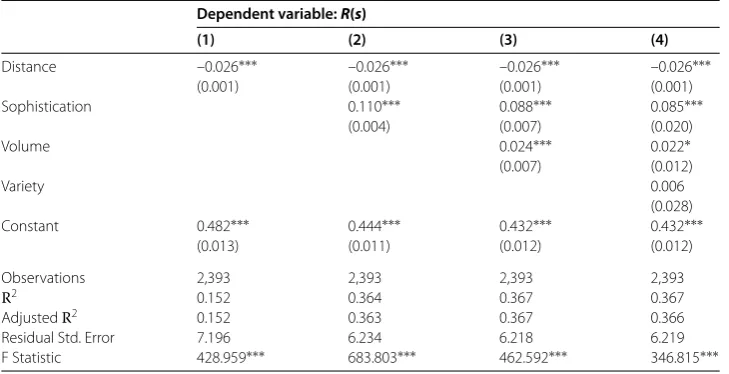
Table 1 Explaining retention with shop distance and size
Dependent variable:R(s)
(1) (2) (3) (4)
Distance –0.026∗∗∗ –0.026∗∗∗ –0.026∗∗∗ –0.026∗∗∗
(0.001) (0.001) (0.001) (0.001)
Sophistication 0.110∗∗∗ 0.088∗∗∗ 0.085∗∗∗
(0.004) (0.007) (0.020)
Volume 0.024∗∗∗ 0.022∗
(0.007) (0.012)
Variety 0.006
(0.028)
Constant 0.482∗∗∗ 0.444∗∗∗ 0.432∗∗∗ 0.432∗∗∗
(0.013) (0.011) (0.012) (0.012)
Observations 2,393 2,393 2,393 2,393
R2 0.152 0.364 0.367 0.367
AdjustedR2 0.152 0.363 0.367 0.366
Residual Std. Error 7.196 6.234 6.218 6.219
F Statistic 428.959∗∗∗ 683.803∗∗∗ 462.592∗∗∗ 346.815∗∗∗
∗p< 0.1;∗∗p< 0.05;∗∗∗p< 0.01. Retention rate goes from 0 to 1. Distance is calculated in minutes. The three measures of size (sophistication, volume and variety) are normalized with average 0 and standard deviation 1.
The null hypothesis states that the largest shops in terms of variety and/or volume will retain more customers, and that there is no variance left to explain for the shop’s sophis-tication. In other words, customers just shop preferentially in larger and more variegated shops. However, our theory gives more importance to complex factors such as the shop’s sophistication. We test a series of models that gradually introduce these factors into ex-plaining the retention rate. All variables except distance have been normalized, fixing their average to and their standard deviation to , so that they are comparable even if dis-tributed on different scales. Table reports the results of our linear model.
First, we examine the effect of distance, calculated in number of minutes. As expected, the further a shop is, the lower the retention rate. SinceR(s) is computed as a share taking values from to , we can say that for each additional minute it takes to reach a shop, we lose two percentage points in the retention rate. If at minutesR(s) equals %, at minutes it is expected to drop to %. The shop’s sophistication plays a significant role: an increase of one standard deviation in sophistication increases the retention rate by percentage points. Disproving the null model, sophistication persists in being significant even accounting for the shop’s volume and variety. In particular, variety is not significant because it is already contained in the sophistication measure, which in turns corrects some of variety’s issues.cNot only sophistication is significant, but its effect size also dominates the others.
4.2 Retention and catch rates facts
We now turn to describing the retention and catch rates for the different shop types. In all the following figures we always report on thexaxis the progressive distance of the shop from the customer and on theyaxis either the retention or the catch rate. BothR(s) and
S(s) are aggregated per shop type. In practice, this means that we collapse all ‘Iper’sinto the single entity ‘Iper’ and the same holds for ‘Super’ and ‘Gestin’.
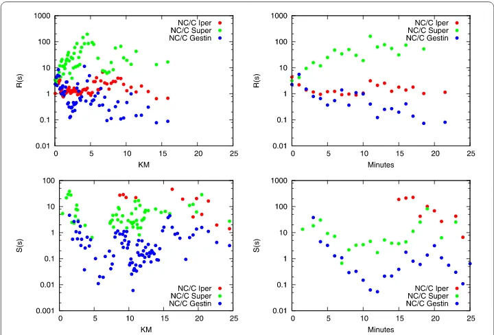
Figure depicts the retention rates for different shop types at progressive spatial (left) and temporal distances (right). Note that the retention power is supposed to be high, as we assume the null hypothesis that the customer should go to the closest shop, choosing a different one only in case of distance ties. Instead, there is a strong difference between the retention power of different types of shops. Larger shops with more sophisticated products (‘Iper’) have the expected attraction power (around % if they are very close, around % when farther). Smaller shops (‘Super’) span from % to % on the same scales. Smallest shops (‘Gestin’) never retain % of the closest customers even if they are literally across the street.
With Figure , we report the catch rates for different shop types, again at progressive distances (spatial on the left, temporal on the right). Note that in the catch rate we are focusing only on customers that have a different shop type as the closest to their home.
Figure 1 Degree of retention per shop type of the closest customers.On thexaxis we have the customer-shop distance, both in kilometres (left) and minutes (right). On theyaxis the share of the customers at the given distance who have that shop as ‘favorite shop’, over all customers at the given distance for which that shop is the closest. We focus only on customers who have that shop as closest, i.e. there is no shop closer than it to the customers (it is allowed to have other shops at the very same distance). Every data point in the plot represents at least 5,000 customers.
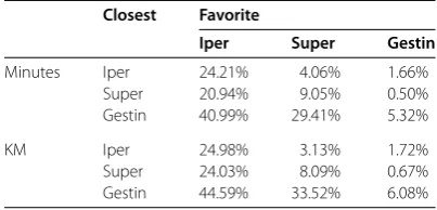
Table 2 Catch rates by shop type
Closest Favorite
Iper Super Gestin
Minutes Iper 24.21% 4.06% 1.66%
Super 20.94% 9.05% 0.50%
Gestin 40.99% 29.41% 5.32%
KM Iper 24.98% 3.13% 1.72%
Super 24.03% 8.09% 0.67%
Gestin 44.59% 33.52% 6.08%
The table counts how many times a customer has as a favorite a shop that is not the closest to her.
The plot describes, for each shop type, the rate of customers attracted that should have chosen to go to a different shop, because closest. Peak catch rates are very different for the different shop types, from ‘Iper’ to ‘Super’ to ‘Gestin’ they respectively stop at -%, -% and -%. Asymptotic behavior is different only for the largest ‘Iper’ shops, resting at around -%. ‘Super’ and ‘Gestin’ do not show significant difference, resting both around % and % respectively. The conclusion from Figures and seems to be that the shop type has a large influence in the customer movement choice. Larger shops retain their closest customer base easily and they can attract significant portions of the customer bases of smaller shops, even at large distances.
In Table , we aggregate the information of the catch rates per shop type presented in Figure . In this case, we add the information about which shop type was the alternative for the customer, i.e. the closest one from which the favorite shop is catching the cus-tomer. Table reports that, for instance, in .% of the cases a customer who had as closest shop (in minutes) a ‘Super’ chose as her favorite shop a ‘Iper’. In .% of the cases, customers who had as closest (in minutes) a ‘Gestin’ chose as favorite a ‘Iper’. The interpretation of the data is that not only the attractive power is proportional to shop’s sophistication (as seen in Figure ), but also this attractive power is more effective the less sophisticated the alternative closest shop is.
4.3 Product-dependent rates
So far we have seen that the shop type plays a significant role in determining whether a customer will choose her closest shop as favorite or not. The result is not surprising: larger shops have greater attractive power. In this section, we present some facts propos-ing a possible motivation. We propose that customers decide to travel farther to larger shops because these shops can offer a larger assortment of more sophisticated products. This is an explanation based on the characteristics of the products that satisfy the needs of the customers, rather than based on other factors. We explore three main product char-acteristics: price, quantity needed and sophistication.
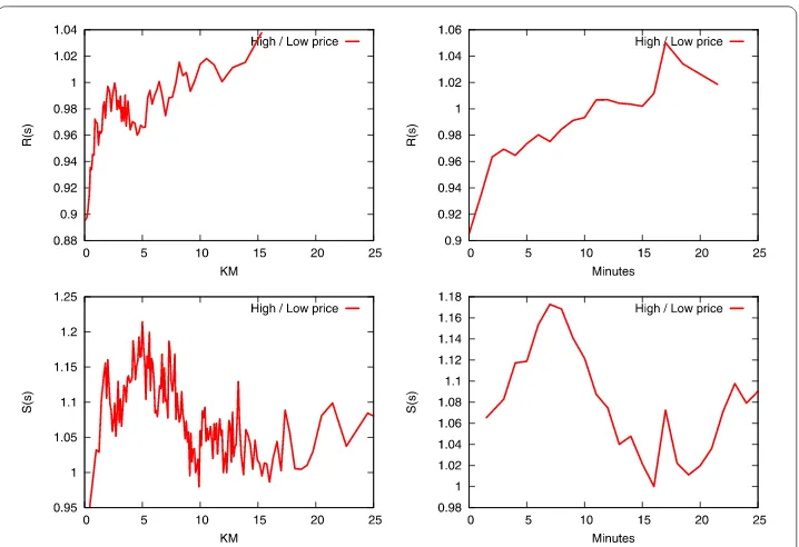
Figure depicts the effect of price on the retention and catch rates. In theyaxis, we con-sider the ratio of high on low price product-seeking customers. A customer is high price seeking set if, in a given shop, she buys mostly products in the high price class (p= ).
She is low price seeking if most of her purchased products in a given shop are from the low price class (p= ). A point on in theyaxis means that customers at a given
Figure 3 Relative degree of retention (top) and catch rate (bottom) per product price type.Same plot as Figures 1 and 2, this time considering all shops together and distinguishing between the two product price classes.
Table 3 Catch rates by shop type for high and low price products
Closest Favorite
High price Low price
Iper Super Gestin Iper Super Gestin
Minutes Iper 24.13% 3.58% 1.59% 24.22% 4.09% 1.67%
Super 23.31% 9.49% 0.38% 20.83% 9.05% 0.52%
Gestin 45.78% 28.60% 4.01% 40.74% 29.51% 5.38%
KM Iper 24.89% 2.71% 1.65% 24.99% 3.16% 1.72%
Super 26.61% 7.91% 0.52% 23.91% 8.13% 0.69%
Gestin 49.57% 32.68% 4.54% 44.31% 33.62% 6.16%
Same as Table 2, but focusing on high and low price products.
given distance from their favorite shop is % larger than the set of low price seeking cus-tomers. This interpretation applies to all figures in this section, substitutingpwithQp
andSpwhere appropriate.
Figure (top) shows that a nearby shop has -% higher likelihood to be the favorite shop of a customer for low price products. A far away shop has % higher likelihood to be the favorite shop of a customer for high price products. Figure (bottom), focuses on the catch rate: if the shop is not the closest, it is more likely to catch customers from closest shops in high price products. This likelihood is around % higher if not too far, and it goes down to % higher for faraway shops. As a conclusion, we say that product price seems to play some role in the choice of the distance to be traveled. Customers are slightly more likely to travel more if they have to buy more expensive products.
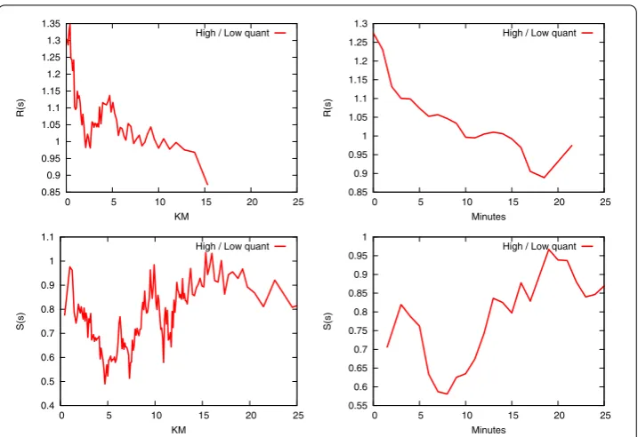
cus-Figure 4 Relative degree of retention (top) and catch rate (bottom) per product quantity type.Same plot as Figure 3, this time distinguishing between products who are bought in large and small quantities.
tomer. The catch rate for high price products for ‘Iper’ shops is higher, while for ‘Super’ and ‘Gestin’ is lower. The opposite holds for low price products. We can confirm that price plays a role when deciding to have a favorite shop.
We now turn our attention to the quantity variable. From Figure (top), we see that a nearby shop has -% higher likelihood to be the favorite shop of a customer for high quantity products. A far away shop has % higher likelihood to be the favorite shop of a customer for low quantity products. Figure (bottom) shows that if the shop is not the closest, it is more likely to catch customers from closest shops in low quantity products. This likelihood is around % higher if not too far, and it goes down to % higher for faraway shops. As a conclusion, we say that product quantity seems to play a significant role in the choice of the distance to be traveled. Both indicators are higher than the price effect discussed in Figure . Customers are more likely to travel more if they have to buy products they need in lower quantities.
We again reinforce this result by splitting the catch rates according to which shop type was the closest to the customer, in Table . The catch rate for low quantity products for ‘Iper’ shops is higher, while for ‘Super’ and ‘Gestin’ is lower. The opposite holds for low quantity products. The differences are larger than the ones seen in Table . On this basis, we conclude that quantity of purchase seems to play a larger role than the unit price when deciding to have a favorite shop.
Table 4 Catch rates by shop type for high and low quantity products
Closest Favorite
High quantity Low quantity
Iper Super Gestin Iper Super Gestin
Minutes Iper 24.21% 4.06% 1.66% 24.39% 3.39% 1.51%
Super 20.90% 9.04% 0.51% 30.39% 12.79% 0.54%
Gestin 40.91% 29.45% 5.34% 53.82% 26.97% 2.57%
KM Iper 24.98% 3.14% 1.72% 25.16% 2.53% 1.57%
Super 23.99% 8.10% 0.68% 34.02% 10.13% 0.66%
Gestin 44.51% 33.55% 6.10% 57.31% 30.59% 2.89%
Same as Table 3, but focusing on high and low quantity products, rather than price.
Figure 5 Relative degree of retention (top) and catch rate (bottom) per product complexity type.
Same plot as Figures 3 and 4 this time distinguishing between high and low complexity products.
goes down to % for faraway shops. As a conclusion, we say that product sophistication seems to play a significant role in the choice of the distance to be traveled. The indicators are comparable to the ones of product quantity seen in Figure , only marginally higher. Customers are more likely to travel more if they have to buy sophisticated products.
Table reports the same rates by splitting them according to the closest shop type. The catch rate for high complexity products for ‘Iper’ shops is higher, while for ‘Super’ and ‘Gestin’ is lower. The opposite holds for low complexity products. The differences are larger than the ones seen in Tables and . We conclude that the complexity of a prod-uct seems to play the largest role, larger than both price and quantity of purchase, when deciding to have a favorite shop.
cus-Table 5 Catch rates by shop type for high and low complexity products
Closest Favorite
High complexity Low complexity
Iper Super Gestin Iper Super Gestin
Minutes Iper 24.27% 2.78% 1.48% 24.21% 4.13% 1.67%
Super 31.22% 12.43% 0.42% 20.67% 9.06% 0.51%
Gestin 55.93% 26.19% 2.02% 40.45% 29.71% 5.41%
KM Iper 25.02% 2.07% 1.54% 24.99% 3.19% 1.72%
Super 35.08% 9.64% 0.54% 23.73% 8.14% 0.68%
Gestin 59.55% 29.91% 2.27% 44.02% 33.84% 6.18%
Same as Tables 3 and 4, but focusing on high and low complexity products.
Figure 6 Relationship between what customers buy in their closest shop and in their favorite shop, when different.In all plots, each dot is a customer. Thexaxis represents the average product characteristics of the products she bought in the closest shop. In theyaxis, we have the same product characteristics of her purchases, this time calculated over the products bought in her favorite shop, when this is not the closest. Point color is proportional to the number of customers sharing the same values. The products characteristics are the product price (top left), the product quantity (top right) and the product complexity (bottom). Product price and quantity are in natural logarithm.
tomer if the closest and the favorite shops are different. Figure depicts the resulting distributions: price on the left, quantity in the middle and sophistication on the right. The plots can be summarized as follows:
• Most customers tend to behave in the same way in their closest and in their favorite shops. The high concentration of data points corresponds to equivalent prices, quantities and sophistications on both axes;
• There is a pervasive L-shaped pattern. This means that the sophisticated customers (and the ones that spend more on average per item) tend to have two wildly different behaviors in the closest and favorite shops. They tend to buy the expensive and sophisticated products only in one of the two shops and use the other one for bulk, not sophisticated purchases.
Our conclusion is that the customers who actually have different behaviors in the closest and in the favorite shop are the ‘extreme’ ones, the one buying products at high sophistica-tion (low quantities, high prices). When a customer instead has a low sophisticasophistica-tion (high quantity, low prices), her behavior does not change between closest and favorite shops.
4.4 Shop survival
We conclude by looking at the relationship between the retention and catch rates of shops, and their success. As reported in the data section, we know whether a shop was closed during our observation period. We then aggregate the data by splitting shops not only ac-cording to their type (‘Iper’, ‘Super’ and ‘Gestin’), but also acac-cording to their status (Closing ‘Iper’, if the ‘Iper’ was closed during our observation period, Non Closing ‘Iper’ if it was not, and so on). We end up with six shop classes, that we analyze as we did in the previous sections.
Figure reports the degrees of retention and of catch rate for the six classes. Instead of reporting all of them directly, we just calculate the rate ratios of Non Closing (NC) versus Closing (C) for the same shop type. We can see that different shop types have very different behaviors.
In Figure (top) we can see that for ‘Super’ the degree of retention of surviving shops is around times higher, for ‘Iper’ is around times higher, while for ‘Gestin’ it ap-pears that the degree of retention of closed shops was actually higher for faraway shops.
Figure (bottom) shows that catch rates are subject to higher variation. For ‘Iper’ shops the catch rate of surviving shop was much higher than for ‘Super’ shops. ‘Gestin’ shops have higher variation, but it averages around (no difference).
As a conclusion, it looks like ‘Super’ shops get closed if they have a lower degree of retention on their closest customers, while ‘Iper’ shops get closed if they have lower catch rates on non-closest customers. ‘Gestin’ shops are harder to describe.
5 Discussion
5.1 Results in context with previous literature
This work is part of the literature effort of creating models of human mobility. In particular, we focus on the mobility of customers in a market environment. How do customers decide when and where to shop? What are the most important factors influencing these choices? This research literature is very prolific and it is touched from a number of approaches. We depart from classical marketing analysis [–] and the classic data mining community [–], to embrace the more systemic view, putting together the social physics approach with the classical Central Place Theory developed in the s []. We do so by collecting a large amount of data about the overall behavior of the retail population as a whole sys-tem and empirically validate the CPT prediction. Namely, we focus on the idea that shops providing a higher order of goods and services, which have a larger range, cause people to be willing to travel longer distances to visit them.
CPT has a long history, not exempt from criticism []. In this paper, we show that CPT’s central idea holds in retail when tested against real world data, which mandate to drop some of the most troubling assumptions. For instance, the geographical space investigated is not boundless, there is no perfect competition, customers do not have the same needs nor the same purchasing power. In fact, we have shown that it is exactly the behavioral difference of customers, the different sophistication of their needs, that drives their will-ingness to travel. Our work is in line with more recent formulations of CPT, which discuss more sophisticated network dynamics [, ] and a relaxation of CPT with overlapping regions of influence []. We are also not the first to test CPT in the retail scenario []. However, this previous literature focuses on a more coarse view of the retail system, with-out investigating the actual micro behavior of each individual customer, which we can and do observe in our work.
Focusing on social physics applied to retail, a classic result shows the high degree of predictability in customer behavior over a long term temporal span []. In our previous work, we proposed the sophistication explanation: customers travel more to satisfy their most sophisticated needs []. This result shows that customers are self-organizing parts of a complex system []. There have been attempts on improving the resolution of the mobility prediction on shorter time scales []. Here we improve over our previous work by using a more realistic measure of customer-shop distance, and investigating deeper implications of shop and product types on customer mobility.
Works like the one presented in this paper and the ones discussed in this section are affected by a number of methodological and ethic issues. As for the methodology, one challenge is the necessity of controlling for place distributions. Cities are not built in a random way and this distribution of interesting hot spots might influence the results []. On the ethics side, we note that the predictability of human movement always carries an identification hazard, as it has been shown multiple times in literature, for example in []. Work has been done to create location-based apps that can ensure the privacy of its users [].
We conclude the literature review by reporting that the human mobility prediction works like the one presented here have a number of different applications. One of the clas-sical application is in disease prevention. To understand how people move, both at a macro and at a micro scale, would empower us to prevent disease outbreaks, or at least to ensure that they can be effectively confined in restricted areas [–]. There are also market applications to improve the way in which citizens are able to use the public transportation infrastructure. A very novel and fast evolving research track studies the dynamics of car sharing and on demand taxi services [, ].
5.2 Strength and limitations of this study
In this study, we improve over previous works on four factors:
• we frame our results in a more coherent theoretical framework, namely the one created with the idea of the Central Place Theory,
• we use a more realistic distance measure to evaluate customer mobility, • we improve the description precision of the customer mobility decision making
process by considering both product and shop characteristics,
• and we provide a description of the logic with which different shop types are pushed out of business.
These are the main strengths of the paper, because they increase the precision and scriptive ability of researchers and market analysts when dealing with the problem of de-scribing human mobility in a market context, and they connect this ability with the Central Place theoretical foundation.
Our study is not exempt from some limitations. The main limitations we see are the following two: the disentanglement of intrinsic shop characteristics and the uncertainty of the actual customer location. We now briefly discuss both.
In the paper we show different dynamics for different shop types. Larger shops (‘Iper’) have higher retention and catch rates, especially against the smallest shops (‘Gestin’). The hypothesis still to be tested is if this effect has anything to do with the shops’ intrinsic power (shops are larger, thus fulfill more needs), or if there are external explanations (larger shops have better infrastructure). We need to integrate our data sources with other information about how people access the shops: do the shops have larger parking lot? Are they better served by public transportation? Are the customers visiting them by car or by foot? These and other questions need to be answered to have a fully controlled experi-ment on customer mobility. Our results partially address these concerns. Given that we find strong product-dependent variables, it means that the object of the purchase is play-ing an effect on customer’s mobility. If infrastructure-type variables would be the only important factor, we would not see the rates we described in this paper.
customers will go to a retail shop after their work day. This would contaminate the results, because the starting location of the retail trip would be different from the one we think it is. However, the noise introduction is minimal. What changes is the origin of the retail trip, but the destination is bounded to always be the same. In any case, the end point of a retail visit is always the customer’s home location.
5.3 Conclusion
In this paper we provided further insights about the mobility of customers in a market system. We made use of actual routes from the customers’ home locations to the shop they visit, along with the actual time it takes to use these routes. On top of this data, we are able to identify, for each customer, what is their closest shop and what is their fa-vorite one, i.e. the one from which they buy most of the products they need. When the two are different, we showed that different shop types have different rates of retaining their closest customers and of attracting customers that are closer to a different shop. We show evidences that these differences in attraction and retention rates are partially ex-plained by the characteristics of the products customers buy: more expensive and more sophisticated products are the ones for which customers travel the most. This is an em-pirical validation of the more modern formulations of the Central Place Theory, where central places are more attractive depending on the variety of needs they can satisfy. We showed that different shop types have a different relationship with their market audi-ence: larger shops are unsuccessful if they cannot attract customers from other nearby shops, while medium size shops are unsuccessful if they cannot retain their nearby cus-tomers.
Our work opens the way to several future developments. First, we need to better estab-lish the relationship between shop size and the quality of the infrastructure surrounding the shop. Larger shops might have better parking lots, being more accessible even if farther away and so on. By controlling for these factors, we can actually evaluate the net effect of product price and sophistication on customer’s mobility decisions. Second, we can move towards the data mining community and use these features in a predictive framework that, given a customer and a product, will be able to suggest the amount of time the customer is willing to invest to obtain the product. There are a number of marketing applications that could benefit both customers and retailers. Finally, we can explore what are the pri-vacy implications of such systems. These applications will have to ensure that the personal information of the customers is never jeopardized.
Competing interests
The authors declare that they have no competing interests.
Authors’ contributions
DP and MC performed research, prepared figures, carried out empirical analysis and wrote the manuscript. All authors designed research and reviewed the manuscript.
Author details
1CID, Harvard University, 79 JFK St, Cambridge, USA.2IMT, P.za San Ponziano 6, Lucca, Italy.3ISTI, CNR, Via G. Moruzzi, 1,
Pisa, Italy.
Acknowledgements
Endnotes
a https://developers.google.com/maps/documentation/directions/.
b At least more reasonable than straight line distance. The few helicopter-owning customers should not skew the
results too much.
c In fact, adding a non-sophisticated product like water increases variety but decreases complexity, and arguably no
customer would decide to travel more because a shop sells also water.
Received: 14 April 2015 Accepted: 28 September 2015 References
1. Krumme C, Llorente A, Cebrian M, Moro E et al (2013) The predictability of consumer visitation patterns. Sci Rep 3:1645
2. Pennacchioli D, Coscia M, Rinzivillo S, Pedreschi D, Giannotti F (2013) Explaining the product range effect in purchase data. In: 2013 IEEE international conference on big data, pp 648-656
3. Pennacchioli D, Coscia M, Rinzivillo S, Giannotti F, Pedreschi D (2014) The retail market as a complex system. EPJ Data Sci 3(1):33
4. Berry BJ, Garrison WL (1958) Recent developments of central place theory. Pap Reg Sci 4(1):107-120
5. Meijers E (2007) From central place to network model: theory and evidence of a paradigm change. Tijdschr Econ Soc Geogr 98(2):245-259
6. Parr JB, Denike KG (1970) Theoretical problems in central place analysis. Econ Geogr 46(4):568-586
7. Hausmann R, Hidalgo C, Bustos S, Coscia M, Chung S, Jimenez J, Simoes A, Yildirim M (2011) In: The atlas of economic complexity. Puritan Press, Hollis
8. Caldarelli G, Cristelli M, Gabrielli A, Pietronero L, Scala A, Tacchella A (2011) Ranking and clustering countries and their products; a network analysis. arXiv:1108.2590
9. Foxall GR (2005) Understanding consumer choice. Palgrave Macmillan, Basingstoke
10. Shen Z-JM, Su X (2007) Customer behavior modeling in revenue management and auctions: a review and new research opportunities. Prod Oper Manag 16(6):713-728. doi:10.1111/j.1937-5956.2007.tb00291.x
11. Underhill P (2000) Why we buy: the science of shopping. Simon & Schuster, New York. http://www.amazon.com/exec/obidos/redirect?tag=citeulike07-20&path=ASIN/0684849143
12. Agrawal R, Imielinski T, Swami AN (1993) Mining association rules between sets of items in large databases. In: SIGMOD international conference, pp 207-216
13. Kocakoç ID, Erdem S (2010) Business intelligence applications in retail business: OLAP, data mining & reporting services. J Inf Knowl Manag 9(2):171-181
14. Li H (2005) Applications of data warehousing and data mining in the retail industry. In: Proceedings of ICSSSM’05. 2005 international conference on services systems and services management, vol 2, pp 1047-1050
15. Taylor PJ, Hoyler M, Verbruggen R (2010) External urban relational process: introducing central flow theory to complement central place theory. Urban Stud 47(13):2803-2818
16. South R, Boots B (1999) Relaxing the nearest centre assumption in central place theory. Pap Reg Sci 78(2):157-177 17. Dennis C, Marsland D, Cockett T (2002) Central place practice: shopping centre attractiveness measures, hinterland
boundaries and the UK retail hierarchy. J Retail Consum Serv 9(4):185-199
18. Schneider CM, Belik V, Couronné T, Smoreda Z, González MC (2013) Unravelling daily human mobility motifs. J R Soc Interface 10(84):20130246
19. Cho E, Myers SA, Leskovec J (2011) Friendship and mobility: user movement in location-based social networks. In: Proceedings of the 17th ACM SIGKDD international conference on knowledge discovery and data mining, pp 1082-1090
20. De Domenico M, Lima A, Musolesi M (2013) Interdependence and predictability of human mobility and social interactions. Pervasive Mob Comput 9(6):798-807
21. Miritello G, Lara R, Moro E (2013) Time allocation in social networks: correlation between social structure and human communication dynamics. In: Temporal networks. Springer, Berlin, pp 175-190
22. Toole JL, Herrera-Yaqüe C, Schneider CM, González MC (2015) Coupling human mobility and social ties. J R Soc Interface 12(105):20141128
23. Amini A, Kung K, Kang C, Sobolevsky S, Ratti C (2014) The impact of social segregation on human mobility in developing and industrialized regions. EPJ Data Sci 3(1):6
24. Noulas A, Scellato S, Lambiotte R, Pontil M, Mascolo C (2012) A tale of many cities: universal patterns in human urban mobility. PLoS ONE 7(5):37027
25. de Montjoye Y-A, Hidalgo CA, Verleysen M, Blondel VD (2013) Unique in the crowd: the privacy bounds of human mobility. Sci Rep 3:1376
26. Sweatt B, Paradesi S, Liccardi I, Kagal L, Pentlandz A (2014) Building privacy-preserving location-based apps. In: 2014 twelfth annual international conference on privacy, security and trust (PST), pp 27-30
27. Bajardi P, Poletto C, Ramasco JJ, Tizzoni M, Colizza V, Vespignani A (2011) Human mobility networks, travel restrictions, and the global spread of 2009 H1N1 pandemic. PLoS ONE 6(1):16591
28. Belik V, Geisel T, Brockmann D (2011) Natural human mobility patterns and spatial spread of infectious diseases. Phys Rev X 1(1):011001
29. Halloran ME, Vespignani A, Bharti N, Feldstein LR, Alexander K, Ferrari M, Shaman J, Drake JM, Porco T, Eisenberg J et al (2014) Ebola: mobility data. Science 346(6208):433
30. Shmueli E, Mazeh I, Radaelli L, Pentland AS, Altshuler Y (2015) Ride sharing: a network perspective. In: Social computing, behavioral-cultural modeling, and prediction. Springer, Berlin, pp 434-439