A Hierarchical Gene-Set Genetic Algorithm

(1)

A Hierarchical Gene-Set Genetic Algorithm

Tzung-Pei Hong

Department of Computer Science and Information Engineering, National University of Kaohsiung, Kaohsiung, Taiwan Email: [email protected]

Min-Thai Wu

Department of Electrical Engineering, National University of Kaohsiung, Kaohsiung, Taiwan Email: [email protected]

Abstract—In this paper, gene sets, instead of individual genes, are used in the genetic process to speed up convergence. A gene-set mutation operator is proposed, which can make several neighboring genes to simultaneously mutate. A gene-set crossover operator is also designed to choose the crossover points at the boundary of gene sets. The proposed gene-set mutation and crossover operators will cause a larger diversity than the conventional ones. A hierarchical gene-set genetic algorithm is then proposed, which uses adjustable gene-set lengths to find final solutions. Different phases of populations use different gene-set lengths to perform the genetic operations. The gene-set length is shortened in half in each phase until the length is 1. Experiments on three problems are also made to show the effectiveness of the proposed gene-set genetic algorithm.

Index Terms—genetic algorithm, chromosome, gene, gene set, crossover, mutation

I. INTRODUCTION

Genetic algorithms (GAs) have become increasingly important to solving difficult problems because they can provide feasible solutions in a limited amount of time. Ref. [9] Holland et al. first proposed this GAs in 1975. GAs have been successfully applied to the fields of optimization [4][10][21][22], machine learning[8][18], neural networks [15][19][25][26], and fuzzy logic controllers [14][31], among others [13][16][17].

When genetic algorithms are used to solve a problem, a representation that describes the problem states must first be defined. An initial population is then generated and three genetic operations (crossover, mutation, and reproduction) are performed to generate the next generation. In the past, a gene was usually regarded as the basic unit for performing crossover and mutation operations. In this paper, gene sets, instead of individual genes, are used in the genetic process. The operation length can thus be logically thought of as the number of

gene sets, which is much shorter than the total chromosome length. The convergence speed can be faster than that in the original GA and the execution time needed can be reduced. Since the gene-set representation is a little different from the current one, the original crossover and mutation operators also need to be modified. A hierarchical gene-set genetic algorithm is then proposed, which uses adjustable gene-set lengths to find final solutions. At beginning, a larger gene-set length is set and the genetic process is run for a fixed number of generations. Then the gene-set length is shortened in half and the genetic process is run again for a fixed number of generations. The same process is repeated until the gene-set length is 1. In this way, the proposed genetic algorithm can search more flexibly in the solution space. Experiments on three problems are also made to show the effectiveness of the proposed genetic algorithm.

The paper is organized as follows. Some related works are reviewed in Section 2. The gene-set genetic representation is proposed and the crossover and mutation operators for this representation are designed in Section 3. The hierarchical gene-set genetic algorithm is proposed in Section 4. Experimental results for showing the performance of the proposed algorithm are described in Section 5. Conclusion and future works are given in Section 6.

II. REVIEW OF RELATED WORKS

(2)

representation used in GA. Each position in a chromosome is a real value. Real-value vectors are especially useful for solving real-value optimization problems. Permutations are a popular representation for some combinatorial optimization problems [7][23][27] [32]. They encode the set of objects into numbers and then arrange them into a chromosome. As to the finite-state representation [1][6][12], it first constructs a state transition table according to the given problems, and then evolve according to the transitive table. This method is used for the environment in which a sequence of states have some implicit relations and must be generated with the relation. In addition, the parse-tree representation [2] [20][24] is often used for evolving executable structures, such as a program. Each chromosome is represented by a parse tree.

After a representation has been chosen for a problem, the genetic process begins. An initial population is generated and three genetic operations (crossover, mutation, and reproduction) are performed to generate the next generation. The simple genetic algorithm uses a single crossover operator and a single mutation operator throughout the entire genetic process. The same procedure is then repeated until the termination criterion is satisfied. The simple genetic algorithm is described as follows.

The Simple Genetic Algorithm:

Step 1: Define a suitable representation for the problem to be solved.

Step 2: Create an initial population of N individuals for evolution.

Step 3: Define a suitable fitness function for the individuals.

Step 4: Perform genetic operations (crossover and mutation) to generate possible offspring.

Step 5: Evaluate the fitness value of each individual. Step 6: Select superior N individuals according to their fitness values.

Step 7: If the termination criterion is not satisfied, go to Step 4; otherwise, stop the algorithm.

The simple genetic algorithm uses several parameters such as population size, crossover probability pcrossoverand

mutation probability pmutation. The crossover operator

usually exchanges some bits between two individuals with probability pcrossover. Valuable information of the

parents can thus be shared among the offspring. The mutation operator is applied to each single individual with a small probability pmutation. The mutation operator

preserves a reasonable level of population diversity and prevents premature convergence to local optima. The values of pcrossover and pmutation are known to critically

affect the behavior and performance of the genetic algorithm[29].

Some researches about dynamical adjustment of crossover and mutation rates were thus proposed. Srinivas and Patnaik proposed the adaptive genetic algorithm (AGA), in which pcrossover and pmutation are varied

according to the fitness values of the solutions [29]. Fogarty used a varying mutation rate and demonstrated that a mutation rate decreasing exponentially over

generations has superior performance [5]. Davis defined five fixed operators to replace the original crossover and mutation operators [3]. The operators that caused generations with better strings were allocated higher probabilities. Hong et al. proposed a dynamic genetic algorithm (DGA), which simultaneously used more than one crossover and mutation operators to generate the next generation. The crossover and mutation ratios changed along with the evaluation results of the respective offspring in the next generation[11]. This paper tries to improve the performance of the genetic algorithms from a different aspect. Gene sets, instead of individual genes, are used and dynamically adjusted in the genetic process to speed up convergence.

Some common crossover operators are multiple-point crossover[28], uniform crossover[30], one-point crossover, substring crossover, etc. They are briefly described as follows.

1. Multi-point crossover method: This method defines a mask to determine which bits should be exchanged between two individuals. For the positions which are 1 on the mask, the parents exchange the corresponding bits.

2. Uniform crossover method: This method defines a mask to determine which bits should be exchanged between two individuals. Bit values of 1 and 0, however, alternative with each other on the mask.

3. One-point crossover method: There is only one bit with value 1 on the mask. That is, the operator randomly selects a single bit within two parents to perform crossover.

4. Substring crossover method: This method changes arbitrary substrings between two individuals. Lengths and positions of these substrings are chosen at random, but are the same for both individuals.

Some common mutation operators are swapping mutation, inversion mutation, and bit-change mutation, among others. They are briefly described as follows :

1. One-point mutation method: This method changes one bit of a chromosome.

2. Swapping mutation method: This method exchanges arbitrary two bits in a chromosome.

3. Inversion mutation method: This method changes the order of the bits in an arbitrary interval of a chromosome.

4. Bit-change mutation method: This method changes the bit value 0 to 1 and 1 to 0 in an entire chromosome.

III. THE GENE-SET REPRESENTATION AND OPERATORS In this paper, the gene-set genetic algorithm is proposed to speed up the convergence of the genetic process. The representation is first described below.

A. Gene-Set Representation

(3)

2a/2b, which is 2a-b. Fig. 2 shows an example in which 8 gene sets are formed from a chromosome with 32 genes.

ngenes

a gene-set

g_n-m₊₁g_n-m₊₂…g_n

… … …

g_m₊₁g_m₊₂…g₂_m g₁g₂…g_m

Figure 1. Gene-set representation

When gene sets, instead of individual genes, are used in the genetic process, the operation length can be logically thought of as the number of gene sets, which is much shorter than the total gene length. The convergence speed is thus faster than that in the original GA, and the execution time needed can be reduced. The experimental results described in Section 5 will show the effect. Note that the gene-set representation can also be easily extended to other gene types in addition to binary bits.

B. The Proposed Gene-Set Mutation Operator

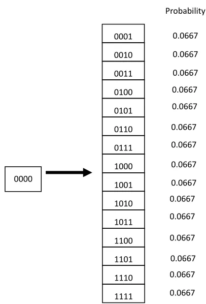
Since the gene-set representation is a little different from current one, the genetic operations must also be modified or re-designed. The gene-set mutation operation is first proposed here. As mentioned above, a gene set is a unit which is operated as a whole. Assume each gene set in a chromosome is chosen for mutation with the probability of pmu. If a gene set has been chosen for

mutation, the proposed mutation operator will convert the original gene set into another possible one with the same probability except itself. For binary-bit genes, the probability can be easily derived as 1/(2m-1), where m is the length of a gene set. Fig. 3 shows an example of the proposed mutation operation for a 4-bits gene set. Assume the gene set “0000” has been chosen for mutation. It may be converted into one of the other 15 different gene sets with the same probability, 0.0667.

Note that the conventional single-point mutation operator sets a mutation rate for each gene. That is, each gene may be mutated from 0 to 1 or vice verse according to the given mutation rate. In this way, the probability for several neighboring genes to simultaneously mutate will be much smaller than that for a single gene. For example, assume the four genes “0000” are to be mutated and the mutation rate is 0.04. Fig. 4 shows that the fifteen possible mutation results with their probability by the conventional single-point mutation operator.

Note that the proposed gene-set mutation operator will assign the same probability to all the possible offspring. It will thus have a larger diversity than the conventional one.

0001 1101 1111 1100 1011 1011 1100 1000

Figure 2. An example of 4-bit gene sets for a chromosome with 32 bits

0000

0001 0010 0011 0100 0101 0110 0111 1000 1001 1010 1011 1100 1101 1110 1111

0.2349 0.2349 0.0098 0.2349 0.0098 0.0098 0.0004 0.2349 0.0098 0.0098

0.0004 0.0098 0.0004 0.0004 0.00002 Probabilityy

Figure 4. The probability distribution from the conventional

single-point mutation operator

0000

0001

0010

0011

0100

0101

0110

0111

1000

1001

1010

1011

1100

1101

1110

1111

0.0667

0.0667 Probability

Figure 3. The mutation operation for a four-bit gene set “0000”.

0.0667

(4)

Figure 6. An example for gradually adjusting gene-set length

1 ~ n Generations

n+1~ 2n Generations

2n+1~ 3n Generations

1011 1111 1000 1010

11 10 11 11 00 10 10 10

1 1 0 1 1 1 1 1 0 0 0 1 0 1 0 1 C. The Proposed Gene-Set Crossover Operator

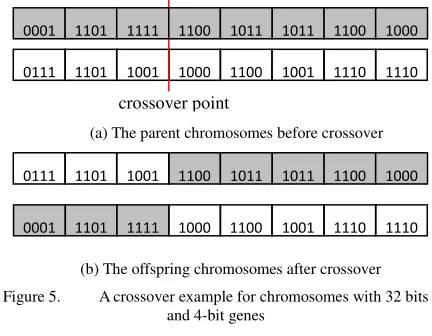
In this paper, a gene-set substring crossover operator is proposed for generating possible offspring. The conventional substring crossover operator exchanges arbitrary substrings between two individuals. In the proposed gene-set substring crossover operator, the crossover points at two parents must be the same and are randomly chosen at the boundary of gene sets. Fig. 5 shows an example for the proposed gene-set crossover operator, and where the crossover point is chosen at the end of the third gene set. The two parent chromosomes in Fig. 5(a) will crossover to produce two possible offspring chromosomes shown in Fig. 5(b).

Note that the average length of the shorter substring in a parent chromosome by the gene-set substring crossover operator will be a little longer than that of the conventional one. For example in a 32-bit chromosome, the gene-set substring crossover will set the crossover point at the boundary. There are thus seven possible crossover points. The average length of the shorter substring for the proposed crossover operation is calculated as (2×(4+8+12)+16)/7, which is 9.1428. The average length of the shorter substring by the original substring crossover operation is (2×(1+2+3+…+15)+16)/ 31, which is 8.2580. It is easily observed that the average length of the shorter substring by the proposed crossover operator is longer than that by the conventional one. The proposed crossover operator will thus in average cause wider discrepancy between offspring and parents.

Formally, let the length of each chromosome is n and the length of each gene set is m. When both n and m are two’s exponential expressions, the number of gene sets will be even. In this case, the average length (AL1)of the

shorter substring by the proposed crossover operator is calculated as follows:

AL1=[(m+2m+…+((n/2)-m)+n/2+((n/2)-m)+((n/2)-2m+

…+m)]/(n/m-1)

= [2×((m+n/2-m)×((n/2)/m-1)/2)+n/2]/(n/m-1) = [(m+n/2-m)×((n/2)/m-1)+n/2]/(n/m-1) = [(n/2×((n/2)/m-1)+n/2)]/ (n/m-1) = ((n/2)2/m)/((n/m)-1)

=(n/2)2/(n-m).

Similarly, the average length (AL2) by the original

crossover operator is calculated as follows:

AL2=[1+2+3+…+(n/2-1)+n/2+(n/2-1)+(n/2-2)+…+] /(n-1)

= [2×((1+n/2-1)×(n/2-1)/2)+n/2]/(n-1) = [(1+n/2-1)×(n/2-1)+n/2]/(n-1) = [n/2×(n/2-1)+n/2]/(n-1) = (n/2)2/(n-1).

The following theorem can then be derived.

Theorem:Let n be the length of each chromosome, m

be the length of each gene set. Assume n and m are two’s exponential expressions, m<n and gcd(m,n)=m. If m>1, the average length of the shorter substring by the proposed gene-set substring crossover operator is longer than that by the original substring crossover operator.

Proof: According to the above derivation, the average

length of the shorter substring by the proposed crossover operator is (n/2)2/(n-m), and is (n/2)2/(n-1) by the original one. If m>1, then n-m<n-1. Thus, (n/2)2/(n-m) >(n/2)2/(n-1).

IV. THE HIERARCHICAL GENE-SET GENETIC ALGORITHM

A genetic process is rough when the gene-set length is large as the entire large gene set is processed as a whole. It is thus suitable to the beginning of a genetic process. On the contrary, the genetic process can be refined if the length is set at a small value. A hierarchical gene-set genetic algorithm is thus proposed here to effectively and efficiently find nearly optimal solutions to a problem. At beginning, a larger gene-set length is set, and the genetic process is run for a fixed number of generations (or until convergence). Then the gene-set length is shortened in half and the genetic process is run again for a fixed number of generations (or until convergence). The same process is repeated until the gene-set length is 1. In this way, the proposed genetic algorithm can search more flexibly in the encoding space. Fig. 6 shows a simple example, where the gene-set length is initially set at 4. The genetic process for each gene-set length is run for n

generations. After n generations have been run, the length will be shortened to 2, and then to 1.

The proposed hierarchical gene-set algorithm is described below.

0001 1101 1111

1100 1011 1011 1100 1000 0111 1101 1001 1000 1100 1001 1110 1110 1100 1011 1011 1100 1000

0111 1101 1001

1000 1100 1001 1110 1110 0001 1101 1111

Figure 5. A crossover example for chromosomes with 32 bits and 4-bit genes

crossover point

(a) The parent chromosomes before crossover

(5)

Figure 7. The fitness values along with different generations for Function A

A. The hierarchical gene-set genetic algorithm:

INPUT: A population size P, a chromosome size w, an initial gene-set length l, a mutation rate rm,, a crossover

rate rc, and a number N of generations in each phase.

OUTPUT: A nearly optimal solution.

Step 1: Define a suitable chromosome representation with size w for the problem to be solved.

Step 2: Define a suitable fitness function for evaluating the individuals.

Step 3: Randomly generate a population of P

individuals.

Step 4: Set k = l, where k is used to keep the gene-set length currently being processed.

Step 5: Set n = 1, where n is used to count the number of generations.

Step 6: Execute gene-set crossover and mutation operations on the population.

Step 7: Evaluate the fitness value of each individual. Step 8: Select the superior P individuals according to their fitness values.

Step 9: Set n = n+1.

Step 10: If n < N, repeat Steps 6 to 10; otherwise, do the next step.

Step 11: set k = k/2.

Step 12: If k < 1, stop the algorithm and output the best chromosome in the current generation as the result; otherwise, go to Step 5.

After the process of the hierarchical gene-set genetic algorithm, a nearly optimal solution to the given problem can be found.

V. EXPERIMENTAL RESULTS

This section reports on experiments made to show the performance of the proposed genetic algorithm. They were implemented in C Language on an AMD K7 2300 with the Linux OS. Also presented are experiments made to compare the time required by the proposed genetic algorithm and by the simple genetic algorithm. The following three problems to find the maximum were used for test:

( )

x = −

(

350 − x

)

2 + 500

fA (1)

( ) (

x = x−2.6

) (

× −19−x

) (

× x+56.5

) (

× x−3

)

fB (2)

( )

x x

( )

x

π

f_C ₌ 4_×sin 2 _{for 0 < x < 100 (3)} The first function is a simple one-peak function with only one local (also global) optimal solution. The second one has two peaks, and the third one has multiple peaks. In all the experiments, the chromosome length was 32 and the initial gene-set length was 4. The termination criterion was the generation number, with each phase being run for the same number of generations.

Experiments were first made for Function A. The problem could actually be solved by calculus. It was used here to compare the performance of the proposed approach and the simple GA. Fig. 7 shows the relations between fitness values and generations for Function A, where the mutation rate was set at 0.06, the population

size at 100, and the total generation number at 2100 (each phase has 700 generations).

-8000 -7000 -6000 -5000 -4000 -3000 -2000 -1000 0 1000

0 300 600 900 1200 1500 1800 2100 2400

fi

tn

e

ss

v

a

lu

e

generations

Population size: 100, Mutation rate: 0.06, Function A

HGSGA SGA

It can be observed from Fig. 7 that the fitness values by both the algorithms increased along with the increase of generations. It was quite consistent with the characteristics of GAs. The gene-set size in the proposed approach was long at the beginning generations, which were regarded as a rough optimization phase. In this phase, the offspring generated by HGSGA lacked delicate local search but focused on big escape movement. The fitness of HGSGA was thus worse than that of SGA in this phase. Along with the gene-set size becoming smaller, the local search in HGSGA was performed more and more delicately and the escape effect was still better than that in simple GA. HGSGA thus soon generated better fitness values than SGA. Fig. 8 shows the execution time along with generations by the two algorithms for Function A. The proposed approach needed less computational time than SGA. Experiments were then made for showing the relations between fitness values and termination generations.

0 20 40 60 80 100 120 140

0 350 700 1050 1400 1750 2100

e

x

e

c

u

ti

o

n

t

im

e

(

s

e

c

)

HGSGA SGA

Fig. 9 shows the results for Function A with mutation rate set at 0.06. It shows that the fitness values by both the algorithms increased along with the increase of termination generations. When the number of termination

(6)

Figure 9. The fitness values along with different termination generations for Function A.

generations was small, convergence could not be achieved. HGSGA had a worse effect than SGA since the former had run only 1/3 of total generations for each phase.

-12000 -10000 -8000 -6000 -4000 -2000 0 2000

0 300 600 900 1200 1500 1800 2100 2400

fi

tn

e

ss

v

a

lu

e

generations

HGSGA SGA

But along with the number of termination generations increased, HGSGA generated better fitness values than SGA. The execution time along with termination generations for Function A by the two algorithms is shown in Fig. 10. Fig. 10 indicates that the proposed approach needed less computational time than SGA for different termination generations. Next, experiments were made to show the effect of the mutation rate on the proposed algorithm. The genetic process was terminated at 600 generations.

0 20 40 60 80 100 120 140

0 300 600 900 1200 1500 1800 2100 2400

ex

ec

u

ti

o

n

ti

m

e

(s

ec

)

generations

HGSGA SGA

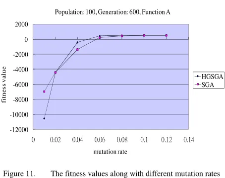
Fig. 11 shows that the final best fitness values along with different mutation rates for Function A by both the two algorithms. It can be observed from Fig. 11 that the fitness value increased along with the increase of the mutation rates. Mutation rates were thus very important to the final results of both the algorithms. The proposed approach needed higher numbers of generations and mutation rates to achieve batter results. Besides, the fitness value of the proposed approach was better than that of the simple GA.

-12000 -10000 -8000 -6000 -4000 -2000 0 2000

0 0.02 0.04 0.06 0.08 0.1 0.12 0.14

fi

tn

e

s

v

a

lu

e

mutation rate

Population: 100, Generation: 600, Function A

HGSGA SGA

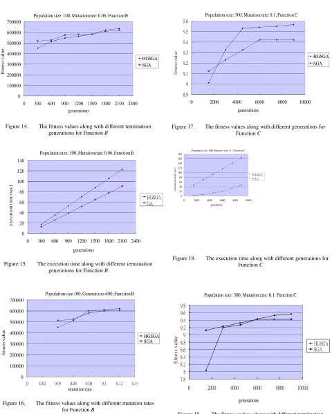
Experimental results for Function B are shown in Figures 12 to 16, which are similar to those for Function

A.

0 100000 200000 300000 400000 500000 600000 700000

0 300 600 900 1200 1500 1800 2100 2400

fi

tn

es

s

v

al

u

e

generations

Population size: 100, Mutation rate: 0.06, Function B

HGSGA SGA

0 20 40 60 80 100 120 140

0 350 700 1050 1400 1750 2100

generations

ex

ec

u

ti

o

n

t

im

e

(s

ec

)

HGSGA SGA

Figure 13. The execution time along with different generations for Function B

Figure 12. The fitness values along with different generations for Function B

Figure 11. The fitness values along with different mutation rates for Function A

(7)

Figure 18. The execution time along with different generations for Function C

0 100000 200000 300000 400000 500000 600000 700000

0 300 600 900 1200 1500 1800 2100 2400

fi

tn

es

s

v

al

u

e

generations

HGSGA SGA

0 20 40 60 80 100 120 140

0 300 600 900 1200 1500 1800 2100 2400

e

x

e

c

u

ti

o

n

t

im

e

(

s

e

c

)

generations

HGSGA GA

0 100000 200000 300000 400000 500000 600000 700000

0 0.02 0.04 0.06 0.08 0.1 0.12 0.14

fi

tn

e

s

v

a

lu

e

mutation rate

Population size 100, Generations 600, Function B

HGSGA SGA

At last, experiments were made for Function C, which is a complex multi-peak function. It has several local optimal solutions. The experimental results are shown in Figures 17 to 21, where the population size was set at 300. The results are also similar to those for the other two functions.

8.9 9 9.1 9.2 9.3 9.4 9.5 9.6

0 2000 4000 6000 8000 10000

fi tn es s v al ue

generations

Population size: 300, Mutation rate: 0.1, Function C

HGSGA SGA

0 20 40 60 80 100 120 140 160 180

0 2000 4000 6000 8000 10000

e

x

e

c

u

ti

o

n

t

im

e

(

se

c

)

generations Population size: 300, Mutation rate: 0.1, Function C

HGSGA SGA

7.88 8.2 8.4 8.6 8.8 9 9.2 9.4 9.6 9.8

0 2000 4000 6000 8000 10000

generations

fi

tn

es

s

v

al

u

e

HGSGA SGA

Figure 19. The fitness values along with different termination generations for Function C.

Figure 17. The fitness values along with different generations for Function C

Figure 16. The fitness values along with different mutation rates for Function B

Figure 15. The execution time along with different termination generations for Function B

(8)

Figure 21. The fitness values along with different mutation rates for Function C

0 20 40 60 80 100 120 140 160 180

0 2000 4000 6000 8000 10000

e

x

e

c

u

ti

o

n

t

im

e

(

s

e

c

)

generations

HGSGA SGA

Population size 300, Generations 9000, Function C

9 9.1 9.2 9.3 9.4 9.5 9.6

0 0.02 0.04 0.06 0.08 0.1 0.12 0.14

mutation rate

fi

tn

es

s

v

al

u

e

(e

+

7

)

HGSGA SGA

VI. Conclusion and Future Works

In this paper, gene sets, instead of individual genes, have been used in the genetic process to speed up the convergence. A gene-set mutation operator has been proposed, which can make several neighboring genes to simultaneously mutate. A gene-set crossover operator has also been designed to choose the crossover points at the boundary of gene sets. The proposed gene-set mutation and crossover operators will cause a larger diversity than the conventional ones.

A hierarchical gene-set genetic algorithm has been proposed, which uses adjustable gene-set lengths to find final solutions. The gene-set length is shortened in half in each phase until the length is 1. In this way, the proposed genetic algorithm can search more flexibly in a solution space. Three problems have been used for experiments, respectively with one-peak, two-peak, and multi-peak solution spaces. From the experimental results, the proposed hierarchical gene-set GA (HGSGA) spends less computational time and gets better fitness values than simple GA. HGSGA can reduce the number of fitness evaluation since the offspring chromosomes generated for gene-sets is smaller than those by the conventional one. Besides, when the termination generations and mutation rates increase, the performance of HGSGA is

significantly improved. In the future, we will attempt to further improve the performance of the proposed approach, such as adding other mechanisms to help the escape from local optimums.

ACKNOWLEDGEMENT

This research was supported by the National Science Council of the Republic of China under contract NSC 96-2213-E-390-003.

REFERENCES

[1] P. J. Angeline and J. B. Pollack, "Evolutionary module acquisition", The Second Annual Conference on Evolutionary programming, pp 154-63, 1993.

[2] P. J. Angeline, "Genetic programming's continued evolution", Advances in Genetic Programming, Vol. 2, MIT Press, pp 1-20, 1996.

[3] L. Davis, "Adapting operator probabilities in genetic algorithms", The Third International Conference on Genetic Algorithms, 1989, pp.61-69.

[4] B. Filipic and D. Juricic, "An interactive genetic algorithm for controller parameter optimization", The International Conference on Artificial Neural Nets and Genetic Algorithms, 1993, pp.458-462.

[5] T. C. Fogarty, "Varying the probability of mutation in genetic algorithms," The Third International Conference on Genetic Algorithms, 1989, pp. 104-109.

[6] L. J. Fogel, A. J. Owens and M. J. Walsh, Artificial Intelligence through Simulated Evolution, Wiley, 1966. [7] B. R. Fox and M. B. McMahon, "Genetic operators for

sequencing problems,” Foundation of Genetic Algorithms, G.. J. E. Rawlins (Ed), Morgan Kaufmann, pp. 284-300, 1991.

[8] D. E. Goldberg, Genetic Algorithms in Search, Optimization & Machine Learning, Addison Wesley, 1989. [9] J. H. Holland. Adaptation in Natural and Artificial Systems,

University of Michigan Press, 1975.

[10]A. Homaifar, S. Guan, and G. E. Liepins, "A new approach on the traveling salesman problem by genetic algorithms," The Fifth International Conference on Genetic Algorithms, 1993, pp.460-466.

[11]T. P. Hong, H. S. Wang, W. Y. Lin and W. Y. Lee, "Evolution of appropriate crossover and mutation operators in a genetic process," Applied Intelligence, Vol. 16, No. 1, 2002, pp. 7-17.

[12]D. Jefferson, R. Collins, C. Cooper, M. Dyer, M. Flowers, R. Korf, C. Taylor and A. Wang, Evolution as a Theme in Artificial Life: the Genesys/Tracker System Artificial Life II, Addison-Wesley, 1991.

[13]D. Jong, "Adaptive system design: a genetic approach," IEEE Transactions on Systems, Man and Cybernetics, Vol. 10, 1980, pp.566-574.

[14]C. L. Karr, "Design of an adaptive fuzzy logic controller using a genetic algorithm," The Fourth International Conference on Genetic Algorithms, 1991, pp.450-457. [15]H. Kitano, "Empirical studies on the speed of convergence

of neural network training using genetic algorithms," The Eighth National Conference on Artificial Intelligence, 1990, pp.789-795.

[16]L. Kuncheva, "Genetic algorithm for feature selection for parallel classifiers," Information Processing Letters, 46, 1993, pp.163-168.

[17]M. A. Lee and H. Takagi, "Dynamic control of genetic algorithms using fuzzy logic techniques," The Fifth Figure 20. The execution time along with different termination

(9)

International Conference on Genetic Algorithms, 1993, pp.76-83.

[18]R. A. McCallum and K. A. Spackman, "Using genetic algorithms to learn disjunctive rules from examples," The Seventh International Conference on Machine Learning, 1990, pp.149-152.

[19]G. F. Miller, P. M. Todd and S. U. Hedge, "Design neural networks using genetic algorithms," The Third International Conference on Genetic Algorithms, 1989, pp.379-384.

[20]D. J. Montana, "Strongly typed genetic programming", Evolutionary Computation, 1995.

[21]T. Munakata and D. J. Hashier, "A genetic algorithm applied to the maximum flow problem," The Fifth International Conference on Genetic Algorithms, 1993, pp.488-493.

[22]P. Prinetto, M. Rebaudengo and M. S. Reorda, "Hybrid genetic algorithms for the traveling salesman problem," The International Conference on Artificial Neural Nets and Genetic Algorithms, 1993.

[23]N. Radcliffe, “Forma analysis and random respectful recombination,” The Fourth International Conference on Genetic Algorithms, R. Belew and L. Booker (Eds), pp. 222-229, 1991.

[24]C. W. Reynolds, "Evolution of obstacle avoidance behavior: using noise to promote robust solutions", Advances in Genetic Algorithms, MIT Press, pp. 221-43, 1994.

[25]P. Robbins, A. Soper and K. Rennolls, "Use of genetic algorithms for optimal topology determination in back propagation neural networks," The International Conference on Artificial Neural Nets and Genetic Algorithms, 1993, pp.726-729.

[26]W. Schiffmann, M. Joost and R. Werner, "Application of genetic algorithms to the construction of topologies for multilayer perceptions," The International Conference on Artificial Neural Nets and Genetic Algorithms, 1993, pp.675-682.

[27]C. Shaefer, "The ARGOT strategy: adaptive representation genetic optimizer technique", The Second International Conference on Genetic Algorithms, pp. 50-58, 1987. [28]W. M. Spears and K. A. Dejong, "An analysis of

multipoint crossover," The Workshop of the Foundations of Genetic Algorithms, 1991, pp. 301-315.

[29]M. Srinivas and L. M. Patnaik, "Adaptive probabilities of crossover and mutation in genetic algorithms," IEEE Transactions on Systems, Man and Cybernetics, Vol. 24, No. 4, 1994, pp.656-666.

[30]G. Syswerda, "Uniform crossover in genetic algorithms," The Third International Conference on Genetic Algorithms, 1989, pp.2-9.

[31]P. Thrift, "Fuzzy logic synthesis with genetic algorithms," The Fourth International Conference on Genetic Algorithms, 1991, pp.509-513.

[32]C. H. Wang, T. P. Hong, S. S. Tseng and C. M. Liao, "Automatically integrating multiple rules sets in a distributed-knowledge environment," IEEE Transactions on Systems, Man, and Cybernetics, Part B, Vol. 28, No. 3, 1998, pp. 471-476.

Tzung-Pei Hong received his B.S. degree in chemical engineering from National Taiwan University in 1985, and his

Ph.D. degree in computer science and information engineering from National Chiao-Tung University in 1992.

He was an associate professor at the Department of Computer Science in Chung-Hua Polytechnic Institute from 1992 to 1994, and at the Department of Information Management in I-Shou University (originally Kaohsiung Polytechnic Institute) from 1994 to 1999. He was a professor in I-Shou University from 1999 to 2001. He was in charge of the whole computerization and library planning for National University of Kaohsiung in Preparation from 1997 to 2000 and served as the first director of the library and computer center in National University of Kaohsiung from 2000 to 2001 and as the Dean of Academic Affairs from 2003 to 2006. He is currently a professor at the Department of Electrical Engineering and at the Department of Computer Science and Information Engineering. He is also the Vice President of National University of Kaohsiung from 2007.

Dr. Hong is a member of the Association for Computing Machinery, the IEEE, the Chinese Fuzzy Systems Association, the Taiwanese Association for Artificial Intelligence, and the Institute of Information and Computing Machinery.

Min-Tai Wu received his B.S degree in the Department of Electrical Engineering from National University of Kaohsiung, Taiwan. He is currently a Ph.D. student in the Department of Computer Science and Engineering, National Sun Yat-sen University, Kaohsiung, Taiwan.