The Complexity of Computing the Optimal Composition of Differential Privacy

www.theoryofcomputing.org

The Complexity of Computing the Optimal

Composition of Differential Privacy

Jack Murtagh

∗

Salil Vadhan

†

Received Month 1, 2012; Revised July 29, 2017; Published June 2, 2018

Abstract: In the study of differential privacy, composition theorems (starting with the original paper of Dwork, McSherry, Nissim, and Smith (TCC’06)) bound the degradation of privacy when composing several differentially private algorithms. Kairouz, Oh, and Viswanath (ICML’15) showed how to compute the optimal bound for composingkarbitrary (ε,δ)-differentially private algorithms. We characterize the optimal composition for the more general case ofkarbitrary(ε1,δ1), . . . ,(εk,δk)-differentially private algorithms where

the privacy parameters may differ for each algorithm in the composition. We show that computing the optimal composition in general is#P-complete. Since computing optimal composition exactly is infeasible (unlessFP=#P), we give an approximation algorithm that computes the composition to arbitrary accuracy in polynomial time. The algorithm is a modification of Dyer’s dynamic programming approach to approximately counting solutions to knapsack problems (STOC’03).

A conference version of this paper appeared in the Proceedings of the 13th IACR Theory of Cryptography Conference

(TCC), 2016-A [14].

∗_{Supported by NSF grant CNS-1237235 and a grant from the Sloan Foundation.}

†_{Supported by NSF grant CNS-1237235, a grant from the Sloan Foundation, and a Simons Investigator Award.}

ACM Classification:F.2

AMS Classification:68Q17, 68W25, 68Q25

1

Introduction

Differential privacy is a framework that allows statistical analysis of private databases while minimizing the risks to individuals in the databases. The idea is that an individual should be relatively unaffected whether he or she decides to join or opt out of a research dataset. More specifically, the probability distribution of outputs of a statistical analysis of a database should be nearly identical to the distribution of outputs on the same database with a single person’s data removed. Here the probability space is over the coin flips of the randomized differentially private algorithm that handles the queries. To formalize this, we call two databasesD0,D1withnrows eachneighboringif they are identical on at leastn−1

rows, and define differential privacy as follows.

Definition 1.1(Differential Privacy [5,4]). A randomized algorithmMis(ε,δ)-differentially privatefor ε,δ ≥0 if for all pairs of neighboring databasesD0andD1and all output setsS⊆Range(M)

Pr[M(D0)∈S]≤eεPr[M(D1)∈S] +δ

where the probabilities are over the coin flips of the algorithmM.

In the practice of differential privacy, we generally think ofε as a small, non-negligible, constant (e. g.,ε =.1). We viewδ as a “security parameter” that is cryptographically small (e. g.,δ =2−30). One of the important properties of differential privacy is that if we run multiple distinct differentially private algorithms on the same database, the resulting composed algorithm is also differentially private, albeit with some degradation in the privacy parameters(ε,δ). In this paper, we are interested in quantifying the degradation of privacy under composition. We will denote the composition ofkdifferentially private algorithmsM1,M2, . . . ,Mkas(M1,M2, . . . ,Mk)where

(M1,M2, . . . ,Mk)(x) = (M1(x),M2(x), . . . ,Mk(x)).

A handful of composition theorems already exist in the literature. The first basic result is the following. Theorem 1.2(Basic Composition [4]). For every ε ≥0, δ ∈[0,1], and (ε,δ)-differentially private algorithms M1,M2, . . . ,Mk, the composition(M1,M2, . . . ,Mk)satisfies(kε,kδ)-differential privacy.

This tells us that under composition, the privacy parameters of the individual algorithms “sum up,” so to speak. We care about understanding composition because in practice we rarely want to release only a single statistic about a dataset. Releasing many statistics may require running multiple differentially private algorithms on the same database. Composition is also a very useful tool in algorithm design. Often, new differentially private algorithms are created by combining several simpler algorithms. Composition theorems help us analyze the privacy properties of algorithms designed in this way.

Theorem 1.3(Advanced Composition [7]). For everyε>0,δ,δ0>0,k∈N,and(ε,δ)-differentially private algorithms M1,M2, . . . ,Mk, the composition(M1,M2, . . . ,Mk)satisfies(εg,kδ+δ0)-differential

privacy for

εg=

p

2kln(1/δ0)·ε+k·ε·(eε−1).

Theorem 1.3shows that privacy under composition degrades by a function ofO(pkln(1/δ0))which is an improvement ifδ0 =2−O(k). It can be shown that a degradation function ofΩ(pkln(1/δ))is necessary even for the simplest differentially private algorithms, such as randomized response [15].

Despite giving an asymptotically correct upper bound for the global privacy parameter,εg, Theo-rem 1.3is not exact. We want an exact characterization because, beyond being theoretically interesting, constant factors in composition theorems can make a substantial difference in the practice of differential privacy. Furthermore,Theorem 1.3only applies to “homogeneous” composition where each individual algorithm has the same pair of privacy parameters,(ε,δ). In practice we often want to analyze the more general case where some individual algorithms in the composition may offer more or less privacy than others. That is, given algorithmsM1,M2, . . . ,Mk, we want to compute the best achievable privacy

parameters for(M1,M2, . . . ,Mk). Formally, we want to compute the following function.

OptComp(M1,M2, . . . ,Mk,δg) =inf{εg≥0 :(M1,M2, . . . ,Mk)is(εg,δg)-DP}.

It is convenient for us to viewδgas given and then compute the bestεg, but the dual formulation,

viewingεgas given, is equivalent (by binary search). Actually, we want a function that depends only on

the privacy parameters of the individual algorithms,

OptComp((ε1,δ1),(ε2,δ2), . . . ,(εk,δk),δg)

=sup{OptComp(M1,M2, . . . ,Mk,δg):Miis(εi,δi)-DP∀i∈[k]}. (1.1)

In other words we want OptComp to give us the minimum possibleεg that maintains privacy for

every sequence of algorithms with the given privacy parameters(εi,δi). A result from Kairouz, Oh, and

Viswanath [12] characterizes OptComp for the homogeneous case.

Theorem 1.4(Optimal Homogeneous Composition [12]1). For everyε≥0andδ ∈[0,1), OptComp((ε,δ),(ε,δ), . . . ,(ε,δ)

| {z }

k

,δg)

equals the least value ofεg≥0such that

1 (1+eε₎k

k

∑

`=lεg_2ε+kεm

k

`

e`ε<sub>−e</sub>εg<sub>e</sub>(k−`)ε_≤1− 1−δg (1−δ)k.

1_{The phrasing ofTheorem 1.4is not exactly how it is presented in [12] (which only refers to}

εgof the form(k−2i)εfor

Empirically (see Section 6), this optimal bound provides a 30-40% savings in εg compared to Theorem 1.3(and a 20% savings compared to an improved asymptotic bound from [12]). The problem remains to find the optimal composition behavior for the more general heterogeneous case. Kairouz, Oh, and Viswanath also provide an upper bound for heterogeneous composition that generalizes the O(pkln(1/δ0))degradation found inTheorem 1.3for homogeneous composition but do not comment on how close it is to optimal.

1.1 Our results

We begin by extending the results of Kairouz, Oh, and Viswanath [12] to the general heterogeneous case. Theorem 1.5(Optimal Heterogeneous Composition). For allε1, . . . ,εk ≥0andδ1, . . . ,δk,δg∈[0,1),

OptComp((ε1,δ1),(ε2,δ2), . . . ,(εk,δk),δg)equals the least value ofεg≥0such that

1

∏ki=1(1+eεi)S⊆{

∑

1,...,k} max

ei∑∈S

εi

−eεg_·ei∑6∈S

εi ,0

≤1− 1−δg

∏ki=1(1−δi)

. (1.2)

Theorem 1.5exactly characterizes the optimal composition behavior for any arbitrary set of differen-tially private algorithms. It also shows that optimal composition can be computed in time exponential in kby computing the sum overS⊆ {1, . . . ,k}by brute force. Of course in practice an exponential-time algorithm is not satisfactory for large k. Our next result shows that this exponential complexity is necessary.

Theorem 1.6. ComputingOptCompis#P-complete, even on instances whereδ1=δ2=· · ·=δk=0

and∑i∈[k]εi≤ε for any desired constantε>0.

Recall that#P is the class of counting problems associated with decision problems in NP. So being#P-complete means that there is no polynomial-time algorithm for OptComp unless there is a polynomial-time algorithm for counting the number of satisfying assignments of Boolean formulas (or equivalently for counting the number of solutions of allNPproblems). So there is almost certainly no efficient algorithm for OptComp and therefore no analytic solution. Despite the intractability of exact computation, we show that OptComp can be approximated efficiently.

Theorem 1.7. There is a polynomial-time algorithm that given rational ε1, . . . ,εk≥0,δ1, . . .δk,δg∈

[0,1),andη∈(0,1), outputsε∗satisfying

OptComp((ε1,δ1), . . . ,(εk,δk),δg)≤ε∗≤OptComp((ε1,δ1), . . . ,(εk,δk),e−η/2·δg) +η.

The algorithm runs in time

O

k3·ε·(1+ε)

η

·log

k2·ε·(1+ε)

η

Note that we incur a relative error ofηin approximatingδgandan additive error ofηin approximating

εg. Since we always takeεgto be non-negligible or even constant, we get a very good approximation when

ηis polynomially small or even a constant. Thus, it is acceptable that the running time is polynomial in 1/η.

In addition to the results listed above, our proof ofTheorem 1.5also provides a somewhat simpler proof of the Kairouz-Oh-Viswanath homogeneous composition theorem (Theorem 1.4[12]). The proof in [12] introduces a view of differential privacy through the lens of hypothesis testing and uses geometric arguments. Our proof relies only on elementary techniques commonly found in the differential privacy literature.

Practical application. The theoretical results presented here were motivated by our work on an applied project called “Privacy Tools for Sharing Research Data”2 [10]. We are building a system that will allow researchers with sensitive datasets to make differentially private statistics about their data available through data repositories using the Dataverse3platform [3,13]. Part of this system is a tool that helps both data depositors and data analysts distribute a global privacy budget across many statistics. Users select which statistics they would like to compute and are given estimates of how accurately each statistic can be computed. They can also redistribute their privacy budget according to which statistics they think are most valuable in their dataset. We implemented the approximation algorithm fromTheorem 1.7and integrated it with this tool to ensure that users get the most utility out of their privacy budget.

Utility-theoretic interpretation. As suggested to us by an anonymous referee, another natural perspec-tive on composition is to maximize the “utility”u(M1, . . . ,Mk)provided bykdifferentially private

algo-rithms for a particular set of analysts subject to a global privacy constraint, OptComp(M1, . . . ,Mk,δg)≤εg.

Our results can be interpreted as studying this problem in the special case whereu(M1, . . . ,Mk) =1 if and

only if for everyi∈[k],Miis a “randomized response” algorithm (seeDefinition 3.1) with privacy

param-etersat leastεi,δi(recall that larger privacy parameters generally yield greater accuracy and hence greater

utility). Following [12], we show inLemma 3.2that randomized response achieves the worst-case bound OptComp((ε1,δ1), . . . ,(εk,δk),δg)over all sequences of algorithmsMithat are(εi,δi)-DP. Studying this

utility maximization problem in greater generality is an interesting direction for future work. (See [1,11] for a general study of utility maximization under one-shot differential privacy, without composition.)

2

Technical preliminaries

A useful notation for thinking about differential privacy is defined below.

Definition 2.1. For two discrete random variablesY andZtaking values in the same output spaceS, the

δ-approximate max-divergenceofY andZis defined as follows.

Dδ

∞(YkZ)≡max

S

lnPr[Y∈S]−δ Pr[Z∈S]

.

2_{https://privacytools.seas.harvard.edu/}

Notice that an algorithmMis(ε,δ)differentially private if and only if for all pairs of neighboring databases,D0,D1, we haveDδ∞(M(D0)kM(D1))≤ε. The standard fact that differential privacy is closed

under “post processing” [5,6] now can be formulated as follows. Fact 2.2. If f:S→R is any randomized function, then

Dδ

∞(f(Y)kf(Z))≤D

δ

∞(YkZ).

Adaptive composition. The composition results in our paper actually hold for a more general model of composition than the one described in the introduction. The model is called adaptive composition and was formalized in [7]. We generalize their formulation to the heterogeneous setting where privacy parameters may differ across different algorithms in the composition.

The idea is that instead of runningkdifferentially private algorithms chosen all at once on a single database, we can imagine an adversary adaptively engaging in a “composition game.” The game takes as input a bitb∈ {0,1}and privacy parameters(ε1,δ1), . . . ,(εk,δk). A randomized adversaryA, tries

to learnb throughk rounds of interaction as follows. On thei-th round of the game, Achooses an (εi,δi)-differentially private algorithmMiand two neighboring databasesD(i,0),D(i,1).Athen receives an

outputyi=Mi(D(i,b))where the internal randomness ofMiis independent of the internal randomness of

M1, . . . ,Mi−1. The choices ofMi,D(i,0),andD(i,1)may depend ony0, . . . ,yi−1as well as the adversary’s

own randomness.

The outcome of this game is called theview of the adversary,Vbwhich is defined to be(y1, . . . ,yk)

along with A’s coin tosses. The algorithms Mi and databases D(i,0),D(i,1) from each round can be

reconstructed fromVb. Now we can formally define privacy guarantees under adaptive composition. Definition 2.3. We say that the sequences of privacy parametersε1, . . . ,εk≥0,δ1, . . . ,δk∈[0,1)satisfy

(εg,δg)-differential privacy under adaptive compositionif for every adversaryAwe have

Dδg

∞(V0kV1)≤εg,

whereVbrepresents the view ofAin composition gamebwith privacy parameter inputs (ε1,δ1), . . . ,(εk,δk).

Computing real-valued functions. Many of the computations we discuss involve irrational numbers and we need to be explicit about how we model such computations on finite, discrete machines. Namely when we talk about computing a function f:{0,1}∗→R, what we really mean is computing f to any desired numberqbits of precision. More precisely, givenx,q, the task is to compute a numbery∈_Qsuch that|f(x)−y| ≤1/2q. We measure the complexity of algorithms for this task as a function of|x|+q. In order to reason about the complexity of OptComp, we will also require that the inputs be rational. So when we talk about computing OptComp exactly, we actually mean givenε1, . . . ,εk≥0,δ1, . . . ,δk,δg∈[0,1)

all rational and an integerq, computeε∗such that

|εg−ε∗| ≤ 1 2q

3

Characterization of OptComp

Following [12], we show that to analyze the composition of arbitrary(εi,δi)-DP algorithms, it suffices to

analyze the composition of the following simple variant of randomized response [15].

Definition 3.1([12]). Define a randomized algorithm ˜M_(ε,δ):{0,1} → {0,1,2,3}as follows, setting α=1−δ.

Pr[M˜_(ε,δ)(0) =0] =δ, Pr[M˜(ε,δ)(1) =0] =0 ,

Pr[M˜_(ε,δ)(0) =1] =α·₁₊eε_eε , Pr[M˜(ε,δ)(1) =1] =α·1+1eε ,

Pr[M˜_(ε,δ)(0) =2] =α·₁₊1_eε , Pr[M˜(ε,δ)(1) =2] =α· e ε

1+eε ,

Pr[M˜_(ε,δ)(0) =3] =0 , Pr[M˜_(ε,δ)(1) =3] =δ.

Note that ˜M_(ε,δ)is in fact(ε,δ)-DP. Kairouz, Oh, and Viswanath showed that ˜M_(ε,δ)can be used to simulate the output of every(ε,δ)-DP algorithm on adjacent databases.

Lemma 3.2([12]). For every(ε,δ)-DP algorithm M and neighboring databases D0,D1, there exists a

randomized algorithm T such that T(M˜_(ε,δ)(b))is identically distributed to M(Db)for b=0and b=1.

For the sake of completeness, we show how this lemma can be deduced from a recent characterization, due to Bun and Steinke [2], of approximate max-divergence as equivalent to exact max-divergence conditioned on events of probability 1−δ.

Lemma 3.3([2]). Let X and Y be random variables. The following are equivalent.

1. Dδ

∞(XkY)≤ε and D

δ

∞(YkX)≤ε.

2. There are probabilistic events E=E(X)and F=F(Y)such that

Pr[E] =Pr[F] =1−δ and D_∞0(X|E kY|F)≤ε and D0∞(Y|F kX|E)≤ε.

3. There are probabilistic events E=E(X)and F=F(Y)such that

Pr[E] =Pr[F]≥1−δ and D0_∞(X|E kY|F)≤ε and D0∞(Y|F kX|E)≤ε.

Bun and Steinke originally provedLemma 3.3usingLemma 3.2, but we give a direct proof here that is in a similar spirit to the proof of an alternate characterization of approximate max-divergence from [7] (which uses statistical distance rather than conditioning on high-probability events). This avoids the need for the hypothesis testing and geometric arguments used in [12] to establish their optimal composition theorem. In an earlier version of our paper, we included a direct proof ofLemma 3.2, without going throughLemma 3.3, but that proof was rather long and tedious, although using similar ideas to the proofs below.

Proof ofLemma 3.3. It is immediate that statement 2 implies statement 3. To see that statement 3 implies

statement 1, note that assuming statement 3, for every setSwe have

Thus we haveDδ

∞(XkY)≤ε and by symmetry we also haveD

δ

∞(YkX)≤ε.

It remains to show that statement 1 implies statement 2, so assume that statement 1 holds. Finding eventsEandFas in statement 2 is equivalent to finding functionseand f such that the following hold.

1. For allx, 0≤e(x)≤Pr[X =x]and 0≤ f(x)≤Pr[Y =x]. 2. For allx,e(x)≤eε_{·f(x)and f(x)≤e}ε_·e(x).

3. ∑xe(x) =∑xf(x) =1−δ.

Indeed, the corresponding eventsE andF are defined by

Pr[E|X=x] =e(x)/Pr[X=x] and Pr[F|Y =x] = f(x)/Pr[Y =x].

Then by Bayes’ Rule, the conditions above imply that

Pr[X=x|E] =Pr[E|X=x]·Pr[X=x]

Pr[E] =

e(x)

∑ye(y)

≤e

ε_·f(x)

∑yf(y) =e

ε_{·Pr[Y =x|F].}

Thus we haveD0_∞(X|E kY|F)≤ε and by symmetry we also haveD0_∞(Y|F kX|E)≤ε.

We now proceed to defining the functionse and f. Define the following disjoint subsets of the domain.

S = {x: Pr[X=x]>eε_{·Pr[Y =x]},} T = {x: Pr[Y =x]>eε_·Pr[X=x]}. Let

α=Pr[X ∈S]−eε·Pr[Y ∈S]≥0 and β =Pr[Y ∈T]−eε·Pr[X ∈T]≥0. We know thatα,β ≤δ, becauseDδ

∞(XkY)≤ε and D

δ

∞(YkX)≤ε. We start by trying to define the

functionseand f as follows.

1. Forx∈S,e(x) =eε_{·Pr[Y =x]and forx∈/S,e(x) =Pr[X=x].} 2. Forx∈T, f(x) =eε_{·Pr[X=x]and forx∈/T, f(x) =Pr[Y =x].}

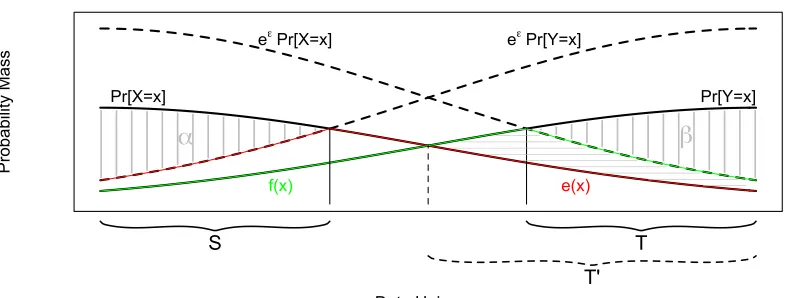
Figure 1shows the functionseand f as defined above as well as the setsSandT and regions whose areas areαandβ. Notice that we have satisfied the conditions

0≤e(x)≤Pr[X=x],

0≤ f(x)≤Pr[Y =x],

e(x)≤eε_{·f(x), and}

f(x)≤eε_·e(x).

Pro

ba

bi

lit

y

Ma

ss

Data Universe eε_Pr[X=x]

Pr[X=x]

eε _Pr[Y=x]

Pr[Y=x]

α

β

f(x) e(x)

S T

T'

Figure 1: Depiction of the functionse(x)(red) and f(x)(green). The solid black curves are the probability mass functions ofX andY and the dashed curves are the solid curves scaled by a factor of eε_{. The regions} with areasα andβ are shaded with vertical lines and the region abovee(x)and below f(x)is shaded with horizontal lines. The setsS,T, andT0from the proof are also depicted.

f(x)over allx, we obtain the following.

∑

x

e(x) =

_∑

x∈S

e(x) +

_∑

x∈/S

e(x)

=

_∑

x∈S

eε_{·Pr[Y=x] +}

∑

x∈/S

Pr[X=x] = eε_{·Pr[Y ∈S] +Pr[X∈/S]} = Pr[X∈S]−α+Pr[X∈/S] = 1−α.

Similarly, we have

∑

x

f(x) =1−β.

Ifα=β=δ, then we’re done. Otherwise, we will modifyeand fto ensure thatα=β and then we will modify them again to achieveα =β =δ. Suppose without loss of generality thatα >β. Then we will reduce the function f on the setT0={x: Pr[Y =x]>Pr[X=x]} ⊇T (seeFigure 1) to reduce the sum

∑x f(x)byα−β (while maintaining all the other conditions). The only condition that might be violated if we reduce the function f is the one thate(x)≤eε_{·f(x). So we just need to confirm that}

∑

x∈T0

is at leastα−β to be able to reduce f as much as we need. We have

∑

x∈T0

(f(x)−e−ε·e(x))≥

_∑

x∈T0

(f(x)−e(x)),

so it suffices to show that the area of the region that is abovee(x)and below f(x)is at leastα−β. To see this, we make the following observations.

1. The area of the region that is above Pr[X =x]and below Pr[Y =x]equals the area of the region that is above Pr[Y =x]and below Pr[X=x].

∑

x∈T0

(Pr[Y =x]−Pr[X=x]) = Pr[Y ∈T0]−Pr[X∈T0]

= (1−Pr[Y ∈/T0])−(1−Pr[X∈/T0])

=

_∑

x∈/T0

(Pr[X=x]−Pr[Y =x]).

(This quantity is simply the total variation distance betweenX andY.)

2. The area of the region that is above Pr[X=x]and below Pr[Y =x]equalsβ plus the area of the region that is abovee(x)and below f(x).

∑

x∈T0

(Pr[Y=x]−Pr[X=x]) =

_∑

x∈T0

(Pr[Y=x]−f(x)) +

_∑

x∈T0

(f(x)−Pr[X=x])

=

_∑

x∈T

(Pr[Y =x]−f(x)) +

_∑

x∈T0

(f(x)−e(x))

= β+

_∑

x∈T0

(f(x)−e(x)).

3. The area of the region that is above Pr[Y =x]and below Pr[X=x]is at leastα.

∑

x∈/T0

(Pr[X=x]−Pr[Y =x]) ≥

_∑

x∈S

(Pr[X=x]−eε_{·Pr[Y =x]} = α.

Putting it all together, we have

∑

x∈T0

(f(x)−e−ε·e(x)) ≥

_∑

x∈T0

(f(x)−e(x))

=

_∑

x∈T0

(Pr[Y =x]−Pr[X=x])−β

≥ α−β.

So we can afford to reduce the sum over allxof f(x)byα−β without violating the other conditions and thus have found two functionseand f such that

2. for allx,e(x)≤eε_{·f(x)and f(x)≤e}ε_·e(x);

3. ∑xe(x) =∑xf(x)≥1−δ.

Suppose∑xe(x) =∑xf(x) =1−δ0>1−δ. Then we can scale them both by a multiplicative factor of

(1−δ0)/(1−δ)and achieve all the desired conditions.

Now we can proveLemma 3.2usingLemma 3.3.

Proof ofLemma 3.2. LetM be an(ε,δ)-DP algorithm and letD0,D1 be neighboring databases. Let

X∼M(D0)andY∼M(D1)be random variables and note that

Dδ

∞(XkY)≤ε and D

δ

∞(YkX)≤ε

becauseMis(ε,δ)-DP.Lemma 3.3says that there exist eventsE,F such that

D0_∞(X|E kY|F)≤ε, D0∞(Y|F kX|E)≤ε, and Pr[E] =Pr[F] =1−δ.

LetRbe the output space ofMand fixr∈R. We define the simulating mechanismT:{0,1,2,3} →Ras follows.

Pr[T(0) =r] =Pr[M(D0) =r|¬E],

Pr[T(1) =r] = 1 eε₋₁·(e

ε_Pr[M(D

0) =r|E]−Pr[M(D1) =r|F]),

Pr[T(2) =r] = 1 eε₋₁·(e

ε_Pr[M(D

1) =r|F]−Pr[M(D0) =r|E]),

Pr[T(3) =r] =Pr[M(D1) =r|¬F].

Note that for each input toT, the probabilities of the outputs sum to 1 and are all non-negative because

D0_∞(X|E kY|F)≤ε and D0_∞(Y|F kX|E)≤ε.

So the outputs ofT form a valid probability distribution. We now show that for allr∈R,

Pr[T(M˜_(ε,δ)(0)) =r] =Pr[M(D0) =r].

It follows that

T(M˜_(ε,δ)(0))∼M(D0)

and by symmetry that

which will complete the proof. We use the shorthandPb(r|H) =Pr[M(Db) =r|H]forb∈ {0,1}and any

eventH. Fixr∈R.

Pr[T(M˜_(ε,δ)(0)) =r]

=δ·Pr[T(0) =r] +(1−δ)e ε

1+eε ·Pr[T(1) =r] +

(1−δ)

1+eε ·Pr[T(2) =r] +0 =δ·P0(r|¬E) +

(1−δ)eε e2ε₋₁ ·(e

ε_P

0(r|E)−P1(r|F)) +

(1−δ) e2ε₋₁ ·(e

ε_P

1(r|F)−P0(r|E))

=δ·P0(r|¬E) +

(1−δ)eε e2ε₋₁ ·e

ε_·P

0(r|E)−

(1−δ)

e2ε₋₁ ·P0(r|E) =δ·P0(r|¬E) + (1−δ)·P0(r|E)

=Pr[¬E]·P0(r|¬E) +Pr[E]·P0(r|E)

=Pr[M(D0) =r].

So ˜M_(ε,δ) can simulate any (ε,δ) differentially private algorithm. Since it is known that post-processing preserves differential privacy (Fact 2.2), it follows that to analyze the composition of arbitrary differentially private algorithms, it suffices to analyze the composition of algorithms ˜M_(εi,δi).

Lemma 3.4. For allε1, . . . ,εk≥0,δ1, . . . ,δk,δg∈[0,1),

OptComp((ε1,δ1), . . . ,(εk,δk),δg) =OptComp(M˜(ε1,δ1), . . . ,M˜(εk,δk),δg).

Proof. Since ˜M_(ε1,δ1), . . . ,M˜_(ε

k,δk)are(ε1,δ1), . . . ,(εk,δk)-differentially private, we have

OptComp((ε1,δ1), . . . ,(εk,δk),δg) =sup{OptComp(M1, . . . ,Mk,δg):Miis(εi,δi)-DP∀i∈[k]}

≥OptComp(M˜_(ε1,δ1), . . . ,M˜_(εk,δk),δg).

For the other direction, it suffices to show that for everyM₁, . . . ,Mk that are(ε1,δ1), . . . ,(εk,δk

)-differentially private, we have

OptComp(M1, . . . ,Mk,δg)≤OptComp(M˜(ε1,δ1), . . . ,M˜(εk,δk),δg).

That is,

inf{εg≥0 :(M1, . . . ,Mk)is(εg,δg)-DP} ≤inf{εg≥0 :(M˜(ε1,δ1), . . . ,M˜(εk,δk))is(εg,δg)-DP}.

So suppose(M˜_(ε1,δ1), . . . ,M˜_(ε

k,δk)) is(εg,δg)-DP. We will show that(M1, . . . ,Mk)is also (εg,δg)-DP.

Taking the infimum overεgthen completes the proof.

We know from Lemma 3.2that for every pair of neighboring databasesD0,D1, there must exist

randomized algorithmsT₁, . . . ,Tk such thatTi(M˜(εi,δi)(b)) is identically distributed to Mi(Db) for all

i∈ {1, . . . ,k}. By hypothesis we have Dδg

∞ (M˜(ε1,δ1)(0), . . . ,M˜(εk,δk)(0))k(M˜(ε1,δ1)(1), . . . ,M˜(εk,δk)(1))

Thus byFact 2.2we have

Dδ∞g (M1(D0), . . . ,Mk(D0))k(M1(D1), . . . ,Mk(D1))

=Dδ∞g (T1(M˜(ε1,δ1)(0)), . . . ,Tk(M˜(εk,δk)(0)))k(T1(M˜(ε1,δ1)(1)), . . . ,Tk(M˜(εk,δk)(1)))

≤εg.

Now we are ready to characterize OptComp for an arbitrary set of differentially private algorithms.

Theorem 1.5(restated). For allε1, . . . ,εk≥0andδ1, . . . ,δk,δg∈[0,1),

OptComp((ε1,δ1),(ε2,δ2), . . . ,(εk,δk),δg)

equals the least value ofεg≥0such that

1

∏ki=1(1+eεi)S⊆{

∑

1,...,k} max

ei∑∈S

εi

−eεg_·ei∑6∈S

εi ,0

≤1− 1−δg

∏ki=1(1−δi) .

Proof ofTheorem 1.5. Given(ε1,δ1), . . . ,(εk,δk)andδg, let ˜Mk(b)denote the composition

(M˜_(ε1,δ1)(b), . . . ,M˜_(εk,δk)(b))

and let ˜P_bk(x)be the probability mass function of ˜Mk(b), forb=0 andb=1. ByLemma 3.4, OptComp((ε1,δ1), . . . ,(εk,δk),δg)

is the smallest value ofεgsuch that

δg≥ max Q⊆{0,1,2,3}k

n ˜

P₀k(Q)−eεg_·P˜k 1(Q),P˜

k

1(Q)−eεg·P˜ k 0(Q)

o

.

Since ˜Mis symmetric, we can instead consider the smallest value ofεgsuch that

δg≥ max Q⊆{0,1,2,3}k

n ˜

P₀k(Q)−eεg_·P˜k 1(Q)

o

, (3.1)

without loss of generality. Givenεg, the setS⊆ {0,1,2,3}k that maximizes the right-hand side is

S=S(εg) =

n

x∈ {0,1,2,3}k

P˜₀k(x)≥eεg·P˜₁k(x) o

.

We can further splitS(εg)intoS(εg) =S0(εg)∪S1(εg)with

S₀(εg) =

n

x∈ {0,1,2,3}k

P˜₁k(x) =0 o

,

S1(εg) =

n

x∈ {0,1,2,3}k

P˜₀k(x)≥eεg·P˜₁k(x),and ˜P₁k(x)>0 o

.

Note thatS0(εg)∩S1(εg) =/0. We have

˜

P₁k(S0(εg)) =0 and P˜₀k(S0(εg)) =1−Pr[M˜k(0)∈ {1,2,3}k] =1− k

∏

i=1

So

˜

P₀k(S(εg))−eεgP˜1k(S(εg)) =P˜0k(S0(εg))−eεgP˜1k(S0(εg)) +P˜0k(S1(εg))−eεgP˜1k(S1(εg))

=1−

k

∏

i=1

(1−δi) +P˜0k(S1(εg))−eεgP˜1k(S1(εg)). (3.2)

Now we just need to analyze ˜

P₀k(S1(εg))−eεgP˜₁k(S1(εg)).

Notice thatS₁(εg)⊆ {1,2}k because for allx∈S1(εg), we have ˜P0(x)>P˜1(x)>0. So we can write

˜

P₀k(S1(εg))−eεg·P˜1k(S1(εg))

=

_∑

y∈{1,2}k

max (

∏

i:yi=1

(1−δi)eεi

1+eεi ·

∏

i:yi=2

(1−δi)

1+eεi −e

εg

∏

i:yi=1

(1−δi)

1+eεi ·

∏

i:yi=2

(1−δi)eεi

1+eεi ,0

)

=

k

∏

i=1

1−δi

1+eεi

∑

y∈{0,1}k

max (

e∑ki=1εi

e∑ki=1yiεi

−eεg_·e∑ik=1yiεi_,0

)

. (3.3)

Combining Equations (3.1), (3.2), and (3.3) together yields

δg≥P˜₀k(S0(εg))−eεgP˜₁k(S0(εg)) +P˜₀k(S1(εg))−eεgP˜₁k(S1(εg))

=1−

k

∏

i=1

(1−δi) + ∏ k

i=1(1−δi)

∏ki=1(1+eεi)S⊆{

∑

1,...,k} max

ei∑∈S

εi

−eεg_·ei∑6∈S

εi ,0

.

We have characterized the optimal composition for an arbitrary set of differentially private algorithms (M1, . . . ,Mk)under the assumption that the algorithms are chosen in advance and all run on the same

database. Next we show that OptComp under this restrictive model of composition is actually equivalent under the more general adaptive composition discussed inSection 2.

Theorem 3.5. The privacy parameters ε1, . . . ,εk ≥0, δ1, . . . ,δk ∈[0,1), satisfy (εg,δg)-differential

privacy under adaptive composition forεg,δg≥0if and only if

OptComp((ε1,δ1), . . . ,(εk,δk),δg)≤εg.

Proof. First suppose the privacy parametersε1, . . . ,εk,δ1, . . . ,δksatisfy(εg,δg)-differential privacy under

adaptive composition. Then OptComp((ε1,δ1), . . . ,(εk,δk),δg)≤εg because adaptive composition is

more general than the composition defining OptComp.

Conversely, suppose OptComp((ε1,δ1), . . . ,(εk,δk),δg)≤εg. In particular, this means

OptComp(M˜_(ε1,δ1), . . . ,M˜_(εk,δk),δg)≤εg.

To complete the proof, we must show that the privacy parametersε1, . . . ,εk,δ1, . . . ,δk satisfy(εg,δg

Fix an adversaryA. On each roundi,Auses its coin tossesrand the previous outputsy1, . . . ,yi−1to

select an(εi,δi)-differentially private algorithmMi=M

r,y1,...,yi−1

i and neighboring databases

D0=Dr₀,y1,...,yi−1, D1=Dr₁,y1,...,yi−1.

LetVbbe the view ofAwith the given privacy parameters under composition gamebforb=0 andb=1.

Lemma 3.2tells us that there exists an algorithmTi=T

r,y1,...,yi−1

i such that

Ti(M˜(εi,δi)(b))

is identically distributed toMi(Db)for bothb=0,1 for alli∈[k]. Define ˆT(z1, . . . ,zk)forz1, . . . ,zk ∈

{0,1,2,3}as follows.

1. Randomly choose coinsrforA. 2. Fori=1, . . . ,k,letyi←T

r,y1,...,yi−1

i (zi).

3. Output(r,y1, . . . ,yk).

Notice that

ˆ

T(M˜_(ε1,δ1)(b), . . . ,M˜_(εk,δk)(b)) is identically distributed toVbfor bothb=0,1. By hypothesis we have

Dδ∞g (M˜(ε1,δ1)(0), . . . ,M˜(εk,δk)(0))k(M˜(ε1,δ1)(1), . . . ,M˜(εk,δk)(1))

≤εg.

Thus byFact 2.2we have Dδg

∞ V0kV1

=Dδg

∞ Tˆ(M˜(ε1,δ1)(0), . . . ,M˜(εk,δk)(0))kTˆ(M˜(ε1,δ1)(1), . . . ,M˜(εk,δk)(1))

≤εg.

4

Hardness of OptComp

#Pis the class of all counting problems associated with decision problems inNP. It is a set of functions that count the solutions to someNPproblem. More formally,

Definition 4.1. A function f:{0,1}∗→Nis in the class#Pif there exists a polynomialp:N→Nand a polynomial time algorithmMsuch that for everyx∈ {0,1}∗,

f(x) = n

y∈ {0,1}p(|x|)_{:M(x,y) =1}o .

Definition 4.2. For functions f,g∈#P, we say that f reduces to g(written f ≤g) if there exists a polynomial time algorithmMsuch that for allx∈ {0,1}∗,M(x) = f(x)whenMis given oracle access to

g. That is, evaluations ofgcan be done in one time step.

If a function is#P-hard, then there is no polynomial-time algorithm for computing it unless there is a polynomial-time algorithm for counting the solutions of allNPproblems.

Definition 4.4. A function f is called#P-easy if there is some functiong∈#Psuch that f can be computed in polynomial time given oracle access tog.

If a function is both #P-hard and#P-easy, we say it is#P-complete. In this section we prove

Theorem 1.6.

Theorem 1.6(restated). ComputingOptCompis#P-complete, even on instances whereδ1=δ2=

. . .=δk=0and∑i∈[k]εi≤ε for any desired constantε>0.

Proving that computing OptComp is#P-complete can be broken into two steps: showing that it is

#P-easy and showing that it is#P-hard. Lemma 4.5. Computing OptComp is#P-easy.

Proof. For convenience we will view rational(ε1,δ1), . . . ,(εk,δk)andεgas given arguments to OptComp

and computeδg. Recall that the two versions of OptComp, viewingεgas given and computingδgand

vice versa, are equivalent up to a polynomial factor (just run binary search over values ofδgcomputing

polynomially many bits of precision). So the formulation we choose for the proof will not affect whether OptComp is in#Por not. Recall that in our model of computing real valued functions, we will take another inputqand we will output an approximation ofδgtoqbits of precision in polynomial time using

a#Poracle whereδgsatisfies the following.

1

∏ki=1(1+eεi)

∑

S⊆{1,...,k}

max

ei∑∈S

εi

−eεg_·e ∑ i6∈S

εi ,0

=1− 1−δg

∏ki=1(1−δi) .

Notice that the only part of the expression above that cannot be computed in polynomial time is the summation over subsets of{1, . . . ,k}. If we knew the sum, computingδgwould be easy given our inputs.

We show how to compute the sum in polynomial time using a#Poracle and it follows that computingδg

is#P-easy.

Define f: 2[k]→_Ras

f(S) =max

ei∑∈S

εi

−eεg_·ei∑6∈S

εi ,0

.

f is computable in polynomial time (to any desired precision). Let ˆf be a function computable in polynomial time wherefˆ(S)−f(S)

<1/2q+k for allS. Setm=10q. Now define the functiong: 2[k]× N→ {0,1}as follows.

g(S,n) =

(

1 ifm·_fˆ_(S)≥n,

0 otherwise.

satisfyingg(S,n) =1) is exactlym·fˆ(S)becausegwill output 1 forg(S,1),g(S,2), . . . ,g(S,m·fˆ(S)). So over all possible setsS, the number of solutions as counted by the#Poracle equalsm·∑S⊆[k]fˆ(S).

Dividing this bymgives us the sum up to an additive error of 2k/2q+k=1/2q, which can be used to computeδgtoqbits of precision in polynomial time. This only required one call to a#Poracle. So

computing OptComp is#P-easy.

Next we show that computing OptComp is also#P-hard through a series of reductions. We start with a multiplicative version of the partition problem that is known to be#P-complete by Ehrgott [9]. The problems in the chain of reductions are defined below.

Definition 4.6. #INT-PARTITION is the following problem. Given a setZ={z1,z2, . . . ,zk}of positive

integers, count the partitionsP⊆[k]such that

∏

i∈P

zi−

∏

i6∈P

zi=0.

All of the remaining problems in our chain of reductions take inputs{w1, . . . ,wk}where 1≤wi≤e

is theD-th root of a positive integerzifor alli∈[k]and some positive integerD. All of the reductions we

present actually hold for every positive integerD, includingD=1 (in which case the inputs are integers). However, we will constrainDto be large enough so that our inputs are in the range[1,e]. This is because in the final reduction to OptComp,εi values in the proof are set to ln(wi). We want to show that our

reductions hold for reasonable values of theεiin a differential privacy setting so throughout the proofs

we use thewi∈[1,e]to correspond to theεi∈[0,1]in the final reduction. In fact, we will later state our

reductions as applying to instances where∏iwi≤eε (and hence∑iεi≤ε) for any desiredε>0.

Definition 4.7. #PARTITION is the following problem. Given a positive integer D∈_N and a set W ={w1,w2, . . . ,wk} of real numbers where 1≤w1, . . . ,wk ≤e are D-th roots of positive integers

z₁, . . .zk, count the partitionsP⊆[k]such that

∏

i∈P

wi−

∏

i6∈P

wi=0.

(The real numbersw₁, . . . ,wkare specified in the input byz1, . . . ,zkandDwith the input size being the

combined bit-length of these integers in binary.)

Definition 4.8. #T-PARTITION is the following problem. Given a positive integer D∈_N, a set W={w1,w2. . . ,wk}of real numbers and apositivereal numberT, where 1≤w1, . . . ,wk≤eareD-th

roots of positive integersz₁, . . .zk, andT = 2D

√

t− 2D√

t0_{for two integerst,t}0_{, count the partitionsP⊆[k]} such that

∏

i∈P

wi−

∏

i6∈P

wi=T.

(The real numbersw₁, . . . ,wkandT are specified in the input byz1, . . . ,zk,t,t0andDwith the input size

Definition 4.9. SUM-PARTITION is the following problem. Given a positive integerD∈_Nand a setW={w1,w2, . . . ,wk}of real numbers where 1≤w1, . . . ,wk≤eareD-th roots of positive integers

z1, . . .zk, and a rational numberr>1, find

∑

P⊆[k]

max (

∏

i∈P

wi−r·

∏

i6∈P

wi,0

)

.

(The real numbersw₁, . . . ,wkare specified in the input byz1, . . . ,zkandDwith the input size being the

combined bit-length of these integers and the numerator and denominator ofrin binary.)

Since the output of SUM-PARTITION is irrational, the actual computational problem is defined according to our convention inSection 2for computing real-valued functions. That is, given an additional inputq, compute a numberysuch that

y−

_∑

P⊆[k]

max (

∏

i∈P

wi−r·

∏

i6∈P

wi,0 )

< 1

2q.

We prove that computing OptComp is#P-hard by the following series of reductions.

#INT-PARTITION≤#PARTITION≤#T-PARTITION≤SUM-PARTITION≤OptComp.

Since #INT-PARTITION is known to be#P-complete [9], the chain of reductions will prove that OptComp is#P-hard.

Lemma 4.10. For every constant c>1,#PARTITIONis#P-hard, even on instances where∏iwi≤c.

Proof. Given an instance of #INT-PARTITION, {z1, . . . ,zk}, we show how to find the solution in

polynomial time using a #PARTITION oracle. SetD=dlogc(∏izi)eandwi= D

√

zi∀i∈[k]. Note that

∏iwi= (∏izi)1/D≤c. LetP⊆[k].

∏

i∈P

wi=

_∏

i6∈P

wi ⇐⇒

_∏

i∈P

wi

!D

=

_∏

i6∈P

wi

!D

⇐⇒

_∏

i∈P

zi=

∏

i6∈P

zi.

There is a one-to-one correspondence between solutions to the #PARTITION problem and solutions to the given #INT-PARTITION instance. We can solve #INT-PARTITION in polynomial time with a #PARTITION oracle. Therefore #PARTITION is#P-hard.

Lemma 4.11. For every constant c>1,#T-PARTITIONis#P-hard, even on instances where∏iwi≤c.

Proof. Let c>1 be a constant. We will reduce from #PARTITION, so consider an instance of the

#PARTITION problem,W ={w1,w2, . . . ,wk} of D-th roots of integersz1, . . . ,zk. We may assume ∏iwi≤

√

SetW0=W∪ {wk+1}, wherewk+1=∏ki=1wi. Notice that k+1

∏

i=1

wi≤(

√

c)2=c.

SetT=√wk+1(wk+1−1). Notice thatwk+1= ∏ki=1zi

D1 _{so by setting integers}

t=

k

∏

i=1

zi

!3

and t0=

k

∏

i=1

zi

we get that

T = 2D√

t− 2D√t0

which meets the input requirement for #T-PARTITION. So we can use a #T-PARTITION oracle to count partitionsQ⊆ {1, . . . ,k+1}such that

∏

i∈Q

wi−

∏

i6∈Q

wi=T.

LetP=Q∩ {1, . . . ,k}. We will argue that∏i∈Qwi−∏i6∈Qwi=T if and only if∏i∈Pwi=∏i6∈Pwi,

which completes the proof. There are two cases to consider:wk+1∈Qandwk+16∈Q.

Case 1:wk+1∈Q. In this case, we have

wk+1·

∏

i∈P

wi

!

−

_∏

i6∈P

wi=

∏

i∈Q

wi−

∏

i6∈Q

wi=T =

√

wk+1(wk+1−1)

⇐⇒

_∏

i∈[k]

wi

!

∏

i∈P

wi

!2

−

_∏

i∈[k]

wi=

s

∏

i∈[k]

wi

∏

i∈[k]

wi−1

!

∏

i∈P

wi

!

multiplied by

_∏

i∈P

wi

⇐⇒





∏

i∈P

wi−

s

∏

i∈[k]

wi



 



∏

i∈[k]

wi

∏

i∈P

wi+

s

∏

i∈[k]

wi



=0 factored quadratic in

∏

i∈P

wi

⇐⇒

_∏

i∈P

wi=

s

∏

i∈[k]

wi

⇐⇒

_∏

i6∈P

wi=

∏

i∈P

wi.

So there is a one-to-one correspondence between solutions to the #T-PARTITION instanceW0where wk+1∈Qand solutions to the original #PARTITION instanceW.

Case 2:wk+16∈Q. Solutions now look like

∏

i∈P

wi−

∏

i∈[k]

wi

∏

i6∈P

wi=

s

∏

i∈[k]

wi

∏

i∈[k]

wi−1

!

One way this can be true is ifwi=1 for alli∈[k]. We can check ahead of time if our input setW

contains all ones. If it does, then there are 2k_{−2 partitions that yield equal products (all exceptP= [k]}

andP=/0) so we can just output 2k−2 as the solution and not even use our oracle. The only other way to satisfy the above expression is for

∏

i∈P

wi>

∏

i∈[k]

wi

which cannot happen becauseP⊆[k]. So there are no solutions in the case thatwk+16∈Q.

Therefore the output of the #T-PARTITION oracle onW0 is the solution to the #PARTITION problem. So #T-PARTITION is#P-hard.

For the next two proofs we will make use of the following fact to bound the amount of precision needed when approximating irrational numbers by rational ones in our reductions.

Fact 4.12. For all real numbers y>x and functions f that are differentiable on the interval[x,y],

f(y)−f(x)≥(y−x)· min

z∈(x,y)

f0(z).

Lemma 4.13. For every constant c>1, SUM-PARTITION is #P-hard even on instances where

∏iwi≤c and where there are no partitions S such that

∏

i∈S

wi=r·

_∏

i6∈S

wi.

Proof. We will use a SUM-PARTITION oracle to solve #T-PARTITION given a setW={w₁, . . . ,wk}

ofD-th roots of positive integersz1, . . . ,zk, and a positive real numberT = 2D

√

t− 2D√

t0for integerst,t0 given in the input. Notice that for everyx>0,

∏

i∈P

wi−

∏

i6∈P

wi=x =⇒

∏

i∈P

wi−

∏i∈[k]wi

∏i∈Pwi

=x

=⇒ ∃ j∈Z+such thatpD j−∏i∈[k] wi

D √

j =x.

Above, jmust be a positive integer greater than ∏ki=1zi

1/2

, which tells us that the gap in products from every partition must take a particular form. This means that for a givenDandW, #X-PARTITION can only be non-zero on a discrete set of possible values ofx. So given our #T-PARTITION instance we can find aT0>T such that the above has no solutions forxin the interval(T,T0). Specifically, solve the above quadratic for √D _{j. If j is not an integer, then we know the answer to the #T-PARTITION}

instance is 0, so assume j is an integer and set T0 = √D _j+1−

∏iwi/D

√

j+1. We can also find an interval(T00,T)just belowT where no value ofxin the interval can yield a solution above by setting T00=√D _j−1−

∏iwi/D

√

j−1. We use these discreteness properties twice in the proof. Also notice that these intervals are not too small.

Claim 4.14. T0−T ≥2−poly(n)_{and T−T}00_≥2−poly(n)_{where n is the input length (i. e., the bit-lengths}

Proof of Claim.

T0−T= pD _j+1−∏i∈[k]wi D √

j+1 −

D

p

j+∏i∈√_D[k]wi

j ≥

D

p

j+1−pD _j≥ 1

D(j+1),

where the last inequality follows fromFact 4.12. This final value is only exponentially small because jis upper bounded by∏ki=1zi, which is at most exponentially large in the bit-length

of thezi. A very similar proof shows that(T00,T)is only exponentially small.

This means that we can always find ˆT ∈(T,T0)such that ˆT is rational and can be fully specified with a bit-length that is polynomial in the input length. Fix such a quantity ˆT. For ally>0, define

Py≡

(

P⊆[k]

∏

i∈P

wi−

∏

i6∈P

wi≥y

)

.

Then, sincex-PARTITION has no solutions forx∈(T,T0), (

P⊆[k]

∏

i∈P

wi−

∏

i6∈P

wi=T

) = P

T_\PTˆ

= 1 T





∑

P∈PT_\PTˆ

∏

i∈P

wi−

_∏

i6∈P

wi

!



= 1

T

∑

P∈PT

∏

i∈P

wi−

∏

i6∈P

wi

!

−

_∑

P∈PTˆ

∏

i∈P

wi−

∏

i6∈P

wi

!!

.

We now show how to compute the two sums in the final term using the SUM-PARTITION oracle. We will give the procedure for computing

∑

P∈PT

∏

i∈P

wi−

∏

i6∈P

wi

!

and the case with ˆT will follow by symmetry. The oracle returns a real number, so by our model of computing real valued functions, we will also give the oracle an additional input that specifies the number of bits of precision in its output. Ultimately we only need to approximate each sum to within±T/4. This will give an approximation to the #T-PARTITION problem to within±1/2, thereby solving it by rounding the approximation because the solution will be an integer. We want to set the inputr to the SUM-PARTITION oracle to ber=rT such that for allP⊆[k], we have

∏

i∈P

wi−rT·

∏

i6∈P

wi≥0 ⇐⇒

∏

i∈P

wi−

∏

i6∈P

wi≥T. (4.1)

Takingw=∏i∈[k]wi and thinking ofv=∏i∈Pwi, it suffices that all positive solutions to each of the

following two inequalities are the same. v−rT

w

v ≥0 and v−

w

The positive solutions to the left one are v≥√rTw, and to the right one arev≥(T+

√

T2_+4w)/2.

Setting the right-hand sides equal gives

rT =

T+√T2_+4w2

4w . (4.2)

SincerT might be irrational and SUM-PARTITION takes as input rational values ofr, we need to

find a rationalrthat approximatesrT and preserves the set of solutionsPT. Recall fromClaim 4.14that

there is an (only) exponentially small interval(T00,T)belowT such that for all ¯T ∈(T00,T),PT =PT¯. This translates to a corresponding interval(rT00,r_T)such that for allr∈(r_T00,r_T), Equivalence (4.1) holds.

Furthermore, this interval is also only exponentially small.

Claim 4.15. rT−rT00 ≥2−poly(n) where n is the input length (i. e., the bit-lengths of the integers

z1, . . . ,zk,t,t0).

Proof of Claim. To see this, view rT from Equation (4.2) as a function r(T) of T, and

calculate the derivative.

r0(T) =

T+√T2_+4w2

2w·√T2_+4w . Fact 4.12says that

rT−rT00=r(T)−r(T00)≥

min

z∈(T00_,T)r

0_(z)

·(T−T00)≥(T−T00)·poly(T).

(Recall that 1≤w=∏iwi≤c). This is only exponentially small in the input length by Claim 4.14.

So we can choose a rationalr∈(rT00,r_T)that can be specified with a number of bits that is polynomial

in the input length and preserves

PT=

(

P⊆[k]

∏

i∈P

wi−r·

∏

i6∈P

wi≥0

)

.

However the SUM-PARTITION oracle gives us

∑

P⊆[k]

max (

∏

i∈P

wi−r·

∏

i6∈P

wi,0 )

=

_∑

P∈PT

∏

i∈P

wi−r·

∏

i6∈P

wi

!

,

SUM-PARTITION oracle forrandr0and receive the output

S₁=

_∑

P∈PT

∏

i∈P

wi−r·

∏

i6∈P

wi

!

,

S2=

∑

P∈PT

∏

i∈P

wi−r0·

_∏

i6∈P

wi

!

.

Then the following linear combination ofS1andS2gives us what we want.

r0−1 r0−r ·S1−

r−1

r0−r·S2=

∑

P∈PT

∏

i∈P

wi−

_∏

i6∈P

wi

!

.

Claim 4.16. Computing S1and S2to within±2−poly(n)yields an approximation of

∑

P∈PT

∏

i∈P

wi−

∏

i6∈P

wi

!

to within±T/4.

Proof of Claim. We just need to approximateS1andS2to within

±T

8 · r0−r r0−1

to get the desired precision. This additive error is only exponentially small byClaim 4.15.

Running this whole procedure again for ˆT ∈(T,T0), which we fixed above gives us all the in-formation we need to count the solutions to the #T-PARTITION instance we were given. We can solve #T-PARTITION in polynomial time with four calls to a SUM-PARTITION oracle. Therefore SUM-PARTITION is#P-hard.

Now we prove that computing OptComp is#P-complete.

Proof ofTheorem 1.6. We have already shown that computing OptComp is#P-easy. Here we prove that

it is also#P-hard, thereby proving#P-completeness.

We are given an instanceD,W={w1, . . . ,wk},r∈Q,andqof SUM-PARTITION, where∀i∈[k], wi is theD-th root of a corresponding integer zi, ∏iwi ≤c, and q specifies the desired number of

bits of precision in the output. If we disregard precision, we would like to setεi =ln(wi)∀i∈[k],

δ1=δ2=. . .δk =0 andεg=ln(r). Note that∑iεi=ln(∏iwi)≤ln(c). Since we can takecto be an

arbitrary constant greater than 1, we can ensure that∑iεi≤ε for an arbitraryε>0.

Again we will use the version of OptComp that takesεg as input and outputsδg. After using an

OptComp oracle to findδgwe know the optimal composition Equation (1.2) fromTheorem 1.5is satisfied.

1

∏ki=1(1+eεi)S⊆{

∑

1,...,k} max

ei∑∈S

εi

−eεg_·ei∑6∈S

εi ,0

=1− 1−δg

∏ki=1(1−δi)

Thus we can compute

δg· k

∏

i=1

(1+eεi_{) =}

∑

S⊆{1,...,k}

max

ei∑∈S

εi

−eεg_·e ∑ i6∈S

εi ,0

=

_∑

S⊆{1,...,k} max

(

∏

i∈S

wi−r·

∏

i6∈S

wi,0 )

.

This last expression is exactly the solution to the instance of SUM-PARTITION we were given. Taking precision into account, the input SUM-PARTITION instance has an additional input qthat specifies the desired number of bits of precision in the output and we can only pass OptComp rational values so we will have to approximateεi=ln(wi)for alliandεg=ln(r). Again there is a worry that

when we approximate these values the set of partitionsSthat make

∏

i∈S

wi−r·

∏

i6∈S

wi>0

might change. We want to get enough precision in our inputs so that the set of partitions over which we sum does not change and enough precision so that the output is accurate toqbits. We will calculate the approximations required for each of these two goals separately and the final precision that we use will just be the maximum of the two. We prove that we can achieve both of these goals with the next two claims. Claim 4.17. There exists a polynomial p(n)in the length n of the input (the bit-lengths of z1, . . . ,zk,q, and

the numerator and denominator of r) such that if|wi−w0i| ≤2

−p(n)_{for each i, then the set of partitions S}

satisfying

∏

i∈S

wi−r·

_∏

i6∈S

wi>0

is the same as the set of partitions satisfying

∏

i∈S

w0_i−r·

_∏

i6∈S

w0_i>0.

Proof of Claim. Recall that SUM-PARTITION is#P-hard even on instances where there

are no partitionsSsuch that

∏

i∈S

wi=r·

∏

i6∈S

wi

so we may assume our input instance of SUM-PARTITION has no such partitions and still prove the hardness of OptComp. So to ensure that we have enough precision such that the set over which we sum does not change, we must make the error smaller than the minimum possible (in absolute value) nonzero outcome of

∏

i∈S

wi−r·

∏

i6∈S

wi.

We now bound this quantity. Let

S=

(

S⊆[k]

∏

i∈S

wi6=

∏

i6∈S

wi

)

Sinceris rational,r=a/bfor two integersaandb. Leta0=aDandb0=bD.

min

S∈_S (

∏

i∈S

wi−r·

∏

i6∈S

wi ) =min

S∈_S   

∏

i∈S

zi

!_D1

− a

0

b0

∏

i6∈S

zi

!_D1    ≥min

S∈_S (

∏

i∈S

zi−

a0

b0

∏

i6∈S

zi · 1

D ∏i∈[k]zi

(D−1)/D )

.

Where the last line follows fromFact 4.12applied to the function f(x) =x1/D.

1/

_∏

i∈[k]

zi

!(D−1)/D

is only exponentially small because∏i∈[k]ziis at most exponentially large in the bit-length

of the integersz₁, . . . ,zk. We claim that

∏

i∈S

zi−

a0 b0

∏

_i6∈Szi

is at least 1/b0for allS∈S. FixS∈S.

∏

i∈S

zi−

a0 b0

∏

_i6∈Szi

=h =⇒

b0·

_∏

i∈S

zi−a0·

∏

i6∈S

zi

=h·b0

=⇒ h≥1/b0.

Where the last implication follows because b0·

_∏

i∈S

zi−a0·

∏

i6∈S

zi

is just a difference of integers so the closest nonzero value it can take on is±1.

Claim 4.18. There exists a polynomial p(n)in the length n of the input (the bit-lengths of z1, . . . ,zk,q,

and the numerator and denominator of r) such that if|wi−w0i| ≤2−p(n)for each i, then

∑

S⊆{1,...,k}

max (

∏

i∈S

w0i−r·

∏

i6∈S

w0i,0

)

−

_∑

S⊆{1,...,k} max

(

∏

i∈S

wi−r·

∏

i6∈S

wi,0 )

≤2−q.

Proof of Claim. We will choosep(n) =p₁(n) +p₂(n)wherep₁(n)is the polynomial that

exists fromClaim 4.17andp2(n)will be determined later. Define

S+=

(

S⊆[k]|

_∏

i∈S

wi−r·

∏

i6∈S

wi>0

)

Claim 4.17says that

S+=

(

S⊆[k]|

_∏

i∈S

w0_i−r·

_∏

i6∈S

w0_i>0 )

.

Now we can write

∑

S⊆{1,...,k}

max (

∏

i∈S

w0_i−r·

_∏

i6∈S

w0_i,0 )

−

_∑

S⊆{1,...,k} max

(

∏

i∈S

wi−r·

∏

i6∈S

wi,0 ) =

∑

S∈S+

∏

_i∈S

w0_i−r·

_∏

i6∈S

w0_i !

−

_∑

S∈S+

∏

_i∈S

wi−r·

∏

i6∈S

wi ! =

∑

S∈S+

∏

_i∈S

w0_i−

_∏

i∈S

wi

!

−

_∑

S∈S+

r·

_∏

i6∈S

w0_i−

_∏

i6∈S

wi ! ≤

∑

S∈S+

∏

_i∈S

w0i−

∏

i∈S

wi ! +

∑

S∈S+

r·

_∏

i6∈S

w0i−

∏

i6∈S

wi ! .

Bounding each term in the final expression above by 2−(q+1)then gives us the accuracy we want. We will show directly how to bound the second term and the argument for the first term follows symmetrically. By hypothesis we have that for allS⊆[k],

∏

i6∈S

w0_i≤

_∏

i6∈S

wi+2−p(n)

≤

_∏

i6∈S

1+2−p(n)

wi≤

1+2−p(n) k

·

_∏

i6∈S

wi

and similarly

∏

i6∈S

w0_i≥1−2−p(n) k

·

_∏

i6∈S

wi.

It follows that for allS⊆[k],

1−2−p(n) k

−1

·

_∏

i6∈S

wi≤

_∏

i6∈S

w0_i−

_∏

i6∈S

wi

!

≤

1+2−p(n) k

−1

·

_∏

i6∈S

wi.

Since|S+| ≤2k_{and 1≤}

∏i6∈Swi≤cfor allSwe get

2k·r·

1−2−p(n)

k

−1

· ≤

_∑

S∈S+

r·

_∏

i6∈S

w0i−

∏

i6∈S

wi

!

≤2k·r·

1+2−p(n)

k

−1

·c.

Pickingp2(n)such that p(n) =p1(n) +p2(n)>2k+log(rc) +q+1 then suffices to bound

the absolute value of the sum by 2−(q+1). Repeating the same calculation for

∑

S∈S+

∏

_i∈S

w0_i−

_∏

i∈S

wi

will yield the same approximation except without the factor ofr. So we can bound both terms by 2−(q+1)_{(and therefore their sum by 2}−q_{) by approximating eachw}

i to a precision

that is polynomial inn, which proves the claim.

So by the two claims above we can get an approximation of the SUM-PARTITION instance toq bits of precision in polynomial time with access to an OptComp oracle. Therefore computing OptComp is#P-hard.

5

Approximation of OptComp

Although we cannot hope to efficiently compute the optimal composition for a general set of differentially private algorithms (assumingP6=NPor evenFP6=#P), we show in this section that we can approximate OptComp to arbitrary precision in polynomial time.

Theorem 1.7 (restated). There is a polynomial-time algorithm that given rational ε1, . . . ,εk ≥0,

δ1, . . . ,δk,δg∈[0,1),andη∈(0,1), outputsε∗satisfying

OptComp((ε1,δ1), . . . ,(εk,δk),δg)≤ε∗≤OptComp((ε1,δ1), . . . ,(εk,δk),e−η/2·δg) +η. The algorithm runs in time

O

k3·ε·(1+ε)

η ·log

k2·ε·(1+ε)

η

whereε=∑i∈[k]εi/k, assuming constant-time arithmetic operations.

We proveTheorem 1.7using the following three lemmas:

Lemma 5.1. Given non-negative integers a1, . . . ,ak, B and weights w1, . . . ,wk∈Q, one can compute

∑

S⊆[k]s.t.

∑ i∈S

ai≤B

∏

i∈S

wi

in time O(Bk).

Notice that the constraint inLemma 5.1 is the same one that characterizes knapsack problems. Indeed, the algorithm we give for computing∑S⊆[k]∏i∈Swiis a slight modification of the known

pseudo-polynomial time algorithm for counting knapsack solutions, which uses dynamic programming. Next we show that we can use this algorithm to approximate OptComp.

Lemma 5.2. Given a rationaleε0 _withε

0≥0andε1=a1·ε0, . . . ,εk=ak·ε0,ε∗=a∗·ε0for positive

integers a1, . . . ,ak,a∗ (given as input), and rational δ1, . . .δk,δg∈[0,1), there is an algorithm that

determines whether or notOptComp((ε1,δ1), . . . ,(εk,δk),δg)≤ε∗and runs in time

O k·

k

∑

i=1

ai

!

In other words, if theε values we are given are all integer multiples of someε0where eε0 is rational,

we can determine whether or not the composition of those privacy parameters is(a∗·ε0,δg)-DP in

pseudo-polynomial time, for every positive integera∗. Running binary search over integersa∗, we can find the minimum such integer. Whenε0is small, this gives us a good overestimate of the optimal composition

of the discrete input privacy parameters. This means that given any inputs(ε1,δ1), . . . ,(εk,δk),δgto

OptComp, we can discretize and polynomially bound theεivalues to new valuesεi0for alli∈[k]and use Lemma 5.2to approximate OptComp((ε₁0,δ1), . . . ,(εk0,δk),δg). The next lemma tells us that this is also a

good approximation of OptComp((ε1,δ1), . . . ,(εk,δk),δg).

Lemma 5.3. For allε1, . . . ,εk,c1, . . . ,ck≥0andδ1, . . . ,δk,δg∈[0,1),

OptComp((ε1+c1,δ1), . . . ,(εk+ck,δk),δg)≤OptComp((ε1,δ1), . . . ,(εk,δk),e−c/2·δg) +c

where c=∑ki=1ci.

Next we prove the three lemmas and then show thatTheorem 1.7follows.

Proof ofLemma 5.1. We modify Dyer’s algorithm for approximately counting solutions to knapsack

problems [8]. The algorithm uses dynamic programming. Given non-negative integersa₁, . . . ,ak,B, and

weightsw1, . . . ,wk∈Q, define

F(r,s) =

_∑

S⊆[r]s.t.

∑ i∈S

ai≤s

∏

i∈S

wi.

We want to computeF(k,B), which we can do by tabulatingF(r,s)for(0≤r≤k,0≤s≤B)using the following recursion.

F(r,s) =   

 

1 ifr=0,

F(r−1,s) +wrF(r−1,s−ar) ifr>0 andar≤s,

F(r−1,s) ifr>0 andar>s.

Each cellF(r,s)in the table can be computed in constant time given earlier cellsF(r0,s0) where r0<r. Thus filling the entire table takes timeO(Bk).

Proof ofLemma 5.2. Given a rational eε0 _{≥0 andε}

1=a1·ε0, . . . ,εk=ak·ε0,ε∗=a∗·ε0 for positive

integersa1, . . . ,ak,a∗and rationalδ1, . . .δk,δg∈[0,1)Theorem 1.5tells us that answering whether or not

OptComp((ε1,δ1), . . . ,(εk,δk),δg)≤ε∗

is equivalent to answering whether or not the following inequality holds. 1

∏ki=1(1+eεi)S⊆{

∑

1,...,k} max

ei∑∈S

εi

−eε∗_·ei∑6∈S

εi ,0

≤1− 1−δg

∏ki=1(1−δi)

The right-hand side and∏ki=1(1+eεi)are easy to compute given the inputs (note that eεi is rational for all

i∈[k]because each is an integer power of eε0_{). So in order to check the inequality, we will show how to}

compute the sum. Define

K=

(

T ⊆[k]|

_∑

i6∈T

εi≥ε∗+

∑

i∈T

εi

)

= (

T ⊆[k]|

_∑

i∈T

εi≤ k

∑

i=1

εi−ε∗ !

/2 )

= (

T ⊆[k]|

_∑

i∈T

ai≤B

)

forB= $

k

∑

i=1

ai−a∗

!

/2 %

and observe that by settingT =Sc, we have

∑

S⊆{1,...,k}

max

ei∑∈S

εi

−eε∗_·ei∑6∈S

εi ,0

=

_∑

T∈K

k

∏

i=1

eεi_·

∏

i∈T

e−εi

!

− eε∗_·

∏

i∈T

eεi

!!

.

We can now useLemma 5.1to compute each term separately sinceKis a set of knapsack solutions. Specifically, settingwi=e−εi ∀i∈[k],Lemma 5.1tells us that we can compute∑T⊆[k]∏i∈Twisubject to

∑i∈Tai≤B, which is equivalent to

∑

T∈K

∏

i∈T

e−εi_.

To compute∑T∈K∏i∈Teεi, we instead setwi=eεi and run the same procedure. (Note that eε

∗

= (eε0₎a∗_,

which is rational.) So we can determine whether or not Inequality (5.1) holds. We used the algorithm fromLemma 5.1so the running time is

O(Bk) =O k·

k

∑

i=1

ai

!

.

Proof ofLemma 5.3. Fix ε1, . . . ,εk,c1, . . . ,ck ≥0 and δ1, . . . ,δk,δg ∈[0,1) and let c=∑i∈[k]ci. Let

OptComp((ε1,δ1), . . . ,(εk,δk),e−c/2·δg) =εg. From Equation (1.2) inTheorem 1.5we know

1

∏ki=1(1+eεi)

∑

S⊆{1,...,k}

max

ei∑∈S

εi

−eεg_·e ∑ i6∈S

εi ,0

≤1−1−e

−c/2_·

δg

∏ki=1(1−δi) .

Multiplying both sides by ec/2gives ec/2

∏ki=1(1+eεi)S⊆{

∑

1,...,k} max

ei∑∈S

εi

−eεg_·ei∑6∈S

εi ,0

≤ec/2· 1−1−e

−c/2_·

δg

∏ki=1(1−δi)

!

≤1− 1−δg