MATLAB FOR ENGINEERS- BASICS AND APPLICATIONS

(1)

(2)

(3)

III

MATLAB FOR ENGINEERS- BASICS AND APPLICATIONS

1

Hazim Nasir Ghafil

Hungary -Miskolc – Miskolc University. [email protected]

2

Shaymaa Mahmood Badr Iraq -Najaf – University of Kufa.

(4)

LIST OF CONTENT

Chapter Content Page Number

1. Basics and concepts 1-3

2. Data Type 4-6

3. MATLAB Basics 7-13

4. Arrzay 14-22

5. M Files 23-30

6. Logical and Comparison Operations 31-35

7. Decision 36-42

8. Loops 43-45

9. Function and Anonymous Function 46-50

10. Plotting 51-69

11. Symbolic Computations 70-72

12. Calculus 73-75

13. Solving Equations and Systems 76-86

LIST OF FIGURE

Sl. No. Name of the figure Page No.

1.1. Graphical user interface for MATLAB R2014a. 1

1.2. Workspace window. 2

1.3. Command History window. 2 1.4. Current Folder window. 3

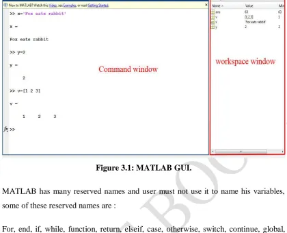
3.1 MATLAB GUI. 8

5.1 New Script button creation. 23

5.2 Run button. 24

5.3 Plotted figure. 26

6.1 The function being called should be in the current folder. 48

10.1 Drawing Line object. 65

10.2 Creating rectangle with sharp corner. 66 10.3 Creating rectangle with curved corners. 66

10.4 Circle scheme. 67

10.5 Circle scheme. 68

(5)

Basics and Concepts World Journal of Engineering Research and Technology

CHAPTER-1

BASICS AND CONCEPTS 1.1 Introduction

MATLAB is acronym of matrix laboratory. It is a high level language powered by several build in function that may need engineers and researchers, MATLAB consider very handy compared with other programming languages like C especially in arithmetical operations.

1.2 graphical user interface GUI

This lecture notes consider MATLAB version R2014a. After installation and starting

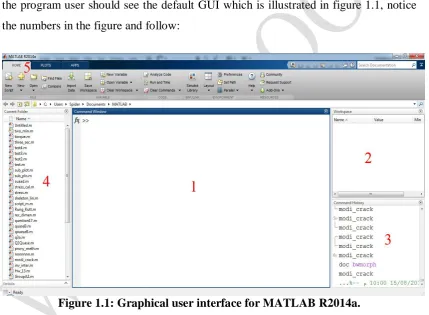
the program user should see the default GUI which is illustrated in figure 1.1, notice the numbers in the figure and follow:

Figure 1.1: Graphical user interface for MATLAB R2014a.

1- Command window

This window where you put your instructions, call functions or commands as well as define variables.

2- Workspace

(6)

double click on the variable name in the Workspace window an excel-like sub window appear containing the numerical values.

Figure 1.2: Workspace window.

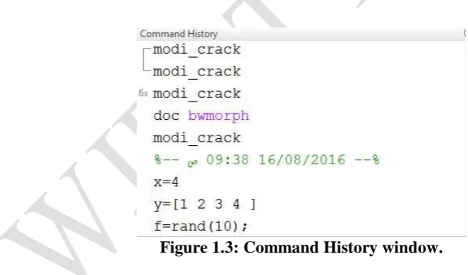
3- Command History

This window shows the last commands used by the user in last sessions and records the time and date at the end of the session, see figure 1.3

Figure 1.3: Command History window.

4- Current Folder

(7)

Basics and Concepts World Journal of Engineering Research and Technology

Figure 1.4: Current Folder window. 1.2 MATLAB tool boxes

MATLAB platform provided with many dedicated tools for a specific scientific field. Users tend to use these tools because they are offer a great deal of facilities and simplify difficult operations that user may need its results without worry about how it really works. We may list some of MATLAB fields operations:

1- Math, Statistics, and Optimization 2- Control Systems

3- Signal Processing and Wireless Communications 4- Image Processing and Computer Vision

5- Test and Measurement 6- Computational Finance 7- Computational Biology

1.3 Simple mathematics

MATLAB enable users to do simple arithmetic operations just like the calculator. These operations called from command window and answer should return by clicking enter button

>> 3+4

(8)

CHAPTER-2 DATA TYPE 2.1 Introduction

In many programming languages users have to declare the type of the variable or and have to state the dimensions of an array. Matlab does not require that. By default, MATLAB stores all numeric variables as double-precision floating-point values, all other types for string, integer etc. will discussed in this chapter.

2.2 Integer and floating-point data

Computer number format are differ from each other by how they stored and how

many bytes occupied in computer memory. Table below lists different data types in MATLAB.

Data type Description

Double Occupies 64 bits in computer memory and represents a wide, dynamic range of values by using a floating point.

Single Occupies 32 bits in computer memory and have less precision and a smaller range.

int8 8-bit signed integer

int16 16-bit signed integer int32 32-bit signed integer

int64 64-bit signed integer

uint8 8-bit unsigned integer

uint16 16-bit unsigned integer uint32 32-bit unsigned integer

uint64 64-bit unsigned integer

True Logical 1

(9)

Data Type World Journal of Engineering Research and Technology

To declare any variable of any type described in above table, use data type name you desire as a function to assign data to the variable

Assign suitable data for a specific data type for example uint16 does not accept negative values, if user do that MATLAB will assign 0 to the variable a instead of the negative number.

2.3 Characters and Strings

In MATLAB char is refer to character data and a vector of it is called string.

Each char type needs 2 bytes to store in computer memory.

(10)

Also user can define char type by holding variable value between two quotations

Now consider this example:

(whos) command return some information about a variables. Notice that x size is 15 which refer to number of characters in x including spaces and occupied size for x in

memory is 30, i.e. 2 byte for each one and x class is char which is mean data type.

2.4 num2str Command

Used to convert number to a string :

y=x/2;

y_val=num2str(y);

2.5 str2num Command

(11)

Matlab Basics World Journal of Engineering Research and Technology

CHAPTER-3 MATLAB BASICS 3.1 Introduction

At the end of this chapter, the reader is expected to know how to define variables, use operators and expressions and work with arrays.

All the matters in this chapter should give reader an ability to write simple programs to solve problems in certain scientific field.

3.2 Variables

Variables refer to a specific area from the memory which hold some value. This value may be any data type we had explained previously.

Variables also can take the form of array and user should take care of the letter case because Matlab is a case sensitive programming language, i.e X differ from x.

3.2.1 Rules of naming variables

There are some rules should obeyed when give a name for a variable

1- The name of the variable must be different from the name of the script file. 2- Start with a letter.

3- It can be consist of more than word divided by underscore. 4- The name of the variable could be up to 63 character.

5- Variable name should not be as the same as name of special variables, we will explain this in section 1.10.

(12)

Figure 3.1: MATLAB GUI.

MATLAB has many reserved names and user must not use it to name his variables, some of these reserved names are :

For, end, if, while, function, return, elseif, case, otherwise, switch, continue, global, break, try, catch.

3.2.2 Special variables

Special variables have some value already reserved by Matlab. the following table describes special ones mostly used.

Special variable Description

pi Ratio of circle circumference to the diameter

Inf Infinity

NaN Not a number

i or j

eps 2.220446049250313*10-16

(13)

We mentioned in section 3.1.2 that user shouldn’t give a names to his variables similar to Matlab special variables, this causes overriding and lost its original value as an example to overriding (pi) value

Restart Matlab will reset special variable to its original values.

3.2.3 clc command

This command cleans the command window of matlab but does not delete variable value from the memory.

3.2.4 clear command

Clear command used to delete variables permanently from the memory and it can be used to clear a specific variable, to do that just type clear followed by variable name in command window

Or you can delete all variables from workspace window by typing only clear in command window

3.2.5 who and whos commands

(14)

3.3 Arithmetic operators

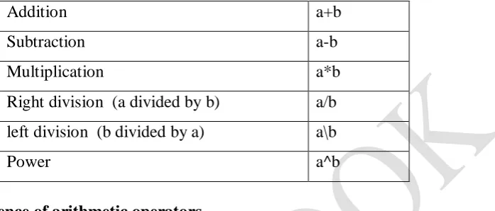
Matlab executes arithmetic operations between two numbers or variables when they written in matlab form. The table below shows the traditional operations.

Table 3.1: Arithmetic operations.

Addition a+b

Subtraction a-b

Multiplication a*b

Right division (a divided by b) a/b

left division (b divided by a) a\b

Power a^b

3.3.1 Precedence of arithmetic operators

A combination of arithmetic operations, such as 2+3*4/5^2, occur in Matlab as the following order :

1- parentheses

2- Power operator executed firstly. 3- Multiplication and division. 4- Addition and subtraction.

Example 3.1

For the expression 2+3*4/5^2*(6+7), Matlab evaluate what inside parentheses (6+7), the expression become

2+3*4/5^2*13 then power operator has been executed so that 2+3*4/25*13 then 3 multiplied by 4

2+12/25*13 Matlab then devide 12 by 25

2+0.48*13 finally 0.48 mutiplied by 13 and the answer added to 2 2+6.24

(15)

It is possible to make Matlab perform 2+3 before other operations just by using parentheses i.e (2+3).

3.4 complex numbers

MATLAB can express complex numbers by means of (i) or (j) which they have

value and do the mathematical operations belong to this type of numbers. Simply complex numbers can be expressed in MATLAB as follows:

Or use j

Mathematical operations can be made for these numbers

(16)

MATLAB also support some useful function relevant to this type of numbers

Function Description

real Return real part of the number imag Return imaginary part of the number

abs Return value of the number

angle Return the angle of the complex number

conj Conjugate of the complex number

3.5 Trigonometric functions

The following table explains trigonometric function used in Matlab

Trigonometric function Explanation

sin(x) Sine function, x in radian

cos(x) Cosine function, x in radian

tan(x) Tangent function, x in radian

cot(x) Cotangent function, x in radian sec(x) Secant function, x in radian

csc(x) Cosecant function, x in radian

sind(x) Sine function, x in degree

cosd(x) Cosine function, x in degree

tand(x) Tangent function, x in degree cotd(x) Cotangent function, x in degree

secd(x) Secant function, x in degree

(17)

To invert any function in the above table just type (a) before trigonometric function such as asin(x) for inverse sine function or acos(x) for inverse cosine function ...etc. Hyperbolic function written as in the following table

Hyperbolic function Explanation

sinh(x) Hyperbolic sine function cosh(x) Hyperbolic cosine function

tanh(x) Hyperbolic tangent function

coth(x) Hyperbolic cotangent function

sech(x) Hyperbolic secant function

csch(x) Hyperbolic cosecant function, asinh(x) Inverse hyperbolic sine function

acosh(x) Inverse hyperbolic cosine function

atanh(x) Inverse hyperbolic tangent function

acoth(x) Inverse hyperbolic cotangent function

asech(x) Inverse hyperbolic secant function

acsch(x) Inverse hyperbolic cosecant function

The following table lists some useful functions

^ power functions Rise to a power exp Exponential function

log Natural logarithm

Log10 Logarithm base 10

Log2 Logarithm base 2 sqrt Square cubic

Approximation functions

All the following resulting in integer numbers

fix Rounds the elements toward zero

floor Round toward negative infinity

ceil Round toward positive infinity

round Round to nearest integer

(18)

CHAPTER-4 ARRAY 4.1 Introduction

Arrays are a sequence of objects arranged in one or more dimensions describe a certain case. In this section we will explain several methods to define a matrices and vectors and introduce mathematical operations that can be applied.

4.2 Vector

You can define a vector of numbers directly by typing in command window a name for the vector then typing its element inside two brackets and separate each other by

comma or space.

4.3 Matrix

Matrix is define by typing row by row separated each other by semicolon [row1; row2; row3…]. Elements of each row separated by comma or space.

4.4 Colon operator

It creates vectors and array subscripting the general expression is

(19)

Array World Journal of Engineering Research and Technology

Also it could be change the step value by the following expression Variable name = start value : step:end value

Step value can be any number positive or negative

4.5 linspace function

It generates a specific equally spaced number of points between to numbers The general expression is

Variable name = lincpace (start value, end value, number of points)

4.6 Semicolon

Writing semicolon at the end of any step or definition prevent the result of that step to show in command window.

(20)

4.7 Calling and modification

It very important to call a specific element, row or column in a matrix. Then you can perform any arithmetic operation on what was called. Matlab very handy to do that.

4.7.1 Call a specific element Let we have a matrix called A

To call any element it must do that by mention its index in the matrix i.e mention its row number and column inside a parentheses. Matlab start indexing from 1 so when it is desired to call 0.1 from matrix A you do that by typing A(1,1)

In the same way when calling element which lay in row 2 and column 3

(21)

4.7.2 Calling row and column

Colon operator was used to call entire row or column. For the matrix A defined previously to call row 2 type A(2,:) this command is read “call all columns in row 2”

Try the command A(:,3) which may be read “call all rows in column 3”.

Also it is possible to call more than one row or column using colon operator

(22)

4.7.3 Delete and change elements

Changing element value in a matrix possible by assign a new value for a specific index for example if it is desired to change 0.1 in matrix A to be 20, just assign the value of 20 the index of 0.1 i.e.

Then Matlab will return matrix A with the newly updated value to the index (1,1). More than that you can assign a new values for entire row or column

(23)

Or linspace to change column 3

(24)

4.7.4 Add a new row or column

Adding a new row or column to a matrix requires attention that the number of the new values match matrix dimension for example to add third column to matrix A you should take consider the A has 2x2 dimensions this mean that the third column must have 2 rows.

(25)

4.8 Array arithmetic operations

Arithmetic operations of matrices and vectors in Matlab is the same as what we learned in mathematics and extra for additional tools.

(26)

The following table describes arithmetic operations that can be applied to an array or between two matrices

Operation Description a+b addition a-b Subtraction

a*b Multiplication

a.*b Element by element multiplication

a/b Left division, this equivalent to the expression inv(b)*a

a./b Element by element division

a\b Right division, this equivalent to the expression inv(a)*b

a^n Power operation where n any positive number. This equivalent to multiplying (a) by itself many times as (n) i.e. for example a^2=a*a

a.^n Each element in matrix a is raised to the power (n) where n any positive number

(27)

M Files World Journal of Engineering Research and Technology

CHAPTER-5 M FILES 5.1 Introduction

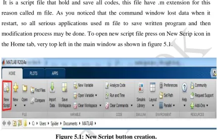
It is a script file that hold and save all codes, this file have .m extension for this reason called m file. As you noticed that the command window lost data when it restart, so all serious applications used m file to save written program and then modification process may be done. To open new script file press on New Scrip icon in the Home tab, very top left in the main window as shown in figure 5.1.

Figure 5.1: New Script button creation.

Or just press Ctrl+n at the keyboard to open new one. User should consider some rules when working with m file 1- File name must not be a name of special function or variable.

2- File name must not be the same as a name of function or variable in the m file itself.

(28)

To run your code, press run in the top tape in editor tab. See figure 5.2.

Figure 5.2: Run button.

5.2 Comment

Matlab executes commands that user input in the script file step by step and the command expression as we learn so far, but in the case of very large code file may be many hundreds of code line it is appear a need to explain some steps or put hints so that any reader can understand what you write in the code.

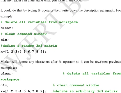
It could do that by typing % operator then write down the description paragraph. For example

% delete all variables from workspace clear;

% clean command window clc;

%define a random 3x3 matrix x=[1 2 3;4 5 6;7 8 9];

Matlab will ignore any characters after % operator so it can be rewritten previous example as:

clear; % delete all variables from workspace

clc; % clean command window

x=[1 2 3;4 5 6;7 8 9]; %define an arbitrary 3x3 matrix

(29)

5.3 disp Command

(disp) command used in m-file to display variable value onto command window. It can display single data

But if it is desired to display multiple objects to command window in single disp command user have to collect all desired objects in one vector.

clear; clc;

x=input('Enter the value of x ');

y=x/2;

y_val=num2str(y);

r='The value of y is equal to '; z=[r,y_val];

disp(z);

5.4 input Command

Used to assign values to a variables in script file by direct input form command window by a user. The default data type for input command is double, for example

x=input('Enter the value of x ');

To assign value of type char use 's' as a set parameter to string

x=input('Enter the value of x ','s');

5.5 Plotting

(30)

Take this example

Where (a) is a vector start with 1 up to 10 with 0.1 as an increment.

b another vector its elements equal to the square of each element in (a) vector.

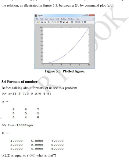
Now by considering (a) as independent variable and (b) as a dependent we can plot the relation, as illustrated in figure 5.3, between a &b by command plot (a,b).

Figure 5.3: Plotted figure. 5.6 Formats of number

Before talking about formats let us see this problem

(31)

Matlab shows number in many formats described in table below. The format function display numbers in command window in a certain style, but do not affect how numbers is saved or calculated in Matlab.

short (default) Short fixed decimal format, with 4

digits after the decimal point. 3.1416

Long

Long fixed decimal format, with 15 digits after the decimal point for double values, and 7 digits after the decimal point for single values.

3.141592653589793

shortE

Short scientific notation, with 4 digits after the decimal point.

Integer-valued floating-point numbers with a maximum of 9 digits do not display in scientific notation.

3.1416e+00

longE

Long scientific notation, with 15 digits after the decimal point for double values, and 7 digits after the decimal point for single values.

Integer-valued floating-point numbers with a maximum of 9 digits do not display in scientific notation.

3.141592653589793e+00

shortG

The more compact of short fixed decimal or scientific notation, with 5 digits.

3.1416

long

The more compact of long fixed decimal or scientific notation, with 15 digits for double values, and 7 digits for single values.

3.14159265358979

shortEng

Short engineering notation, with 4 digits after the decimal point, and an exponent that is a multiple of 3.

3.1416e+000

longEng

Long engineering notation, with 15 significant digits, and an exponent that is a multiple of 3.

3.14159265358979e+000

Bank Currency format, with 2 digits after the decimal point. 3.14

Hex Hexadecimal representation of a binary

(32)

To view the current format type the command get(0,'format')

Now try to change format to long for the previous example

It is clear that b(2,2) equal to a very small number and by set format to short, which is the default one, just 4 digits appear after floating point, so user see an odd value (-0.0000).

Example 5.1

1- A force (P) was applied axially to a circular steel rod of diameter 40 mm. compute the stress in the rod when the applied force raised gradually starting from 1000N up to 20KN, each time force increased by 500N. Finally plot force-stress graph for this

(33)

Answer

clear; clc;

diameter=40*10^-3; % define rod diameter

Force = 1000:500:20000; % assign force range

area = pi/4*(diameter^2); %calculating cross-sectional

area of the rod

stress = Force/area; % computing stress

plot(Force,stress); % plotting force- stress

relation

clear command was used to delete any predefined variables and clc to clean command window to prepare it to show our calculations. The following steps include variables definition i.e. rod diameter and range of applied force. Then cross section area was

calculated to substitute it in the next step which is computing stress at the

(34)

It is clear that the above graph is solid; there are no x or y labels, no hints or information about what we draw. Actually there are more to talk about plotting in MATLAB and will be discussed later.

Example 5.2

Calculate the pressure difference applied on the base of the water tank shown below if the water height increase from 1 to 3 meter with an increment of 0.1 meter

Answer:

clear;

clc;

gamma_water = 9810; % water specific %

weight in N/m3

water_level = 1:0.1:3; % water increased

level in m

pressure = gamma_water*water_level; % pressure applied %

on the tank base in N/m2

(35)

Logical and Comparison Operations World Journal of Engineering Research and Technology

CHAPTER-6

LOGICAL AND COMPARISON OPERATIONS 6.1 Introduction

MATLAB considers, in all logical and comparison operations, any nonzero numbers are true and zero is false. The output of these operations is a logical array contains 1 for true and 0 for false.

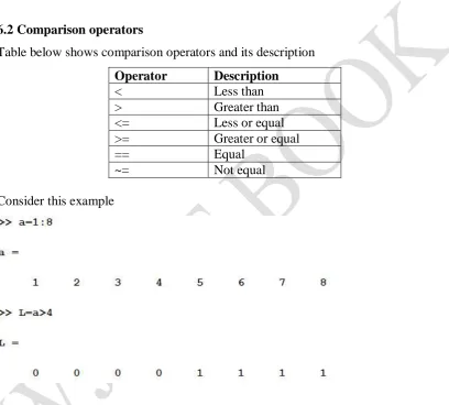
6.2 Comparison operators

Table below shows comparison operators and its description

Operator Description < Less than > Greater than <= Less or equal >= Greater or equal

== Equal

~= Not equal

Consider this example

Where L is a logical vector defined by subjection elements of (a) to the condition (>4). It is clear that the first four elements does not meet the condition therefor it return 0 and the rest of (a) elements meet the condition so, it return 1.

(36)

MATLAB also can performs comparison between two arrays, for example

The operator == test the condition that if any element in (a) is equal to the corresponding element in (b), if they equaled return 1 otherwise return 0.

Mathematical operation can be done between an array and logical array.

6.3 Logical operator

Logical operators offer a way to merge or opposite comparison expressions. The following table show MATLAB logical operators.

Logical operator Description

& AND

| OR

~ NOT

(37)

6.4 logical command

Logical command used to return a logical matrix from numerical one on basis of considering any nonzero element as a true value (one) and zero elements as false value (0)

& (AND) and |(OR) operators work as usual in truth table

& (AND) operator

First value Second value Result

1 1 1

1 0 0

0 1 0

0 0 0

| (OR) operator

First value Second value Result

1 1 1

1 0 1

0 1 1

0 0 0

(38)

6.5 Precedence of logical and comparison operator Consider this expression:

b&w|b

MATLAB does not confused about which operator do first because logical operators run in a precedence like what user know for arithmetic operators.

The following table arrange operators precedence from high to low () Parentheses

< Less than

<= Less than or equal

> Greater than

>= Greater than or equal

== Equal

~= Not equal

& Element-wise logical AND

| Element-wise logical OR

&& Short-circuit logical AND used for scalar values || Short-circuit logical OR used for scalar values

(39)

6.6 Logical Operations

MATLAB supports symbolic expressions which is used for different purposes, these expressions listed in table 6.1.

Expression Description and Logical AND

Syntax: and(A,B)

not Logical NOT Syntax: not(A,B)

Logical OR Syntax: or(A,B)

xor

Logical XOR: performs an exclusive OR operation on the corresponding elements of arrays A and B. The resulting element is logical true if Aor B but not both, is nonzero.

all Check if all the elements in the array are nonzero or true any Check if any of the elements in the array are nonzero or true

(40)

CHAPTER-7 DECISION 7.1 Introduction

User sometimes have to make a decision to choose a specific case among many or changing program stream a according to a condition. MATLAB like many professional programming languages, supported by a decision tools to enable user to make his choice.

7.1 if …end Statement The general expression is

if <logical or comparison operation> Operation

end

Ex1:

write a program to read a number and compares it with (5) and return a sentence show if the entered number is equal to or less or greater than (5).

Solution

(41)

Decision World Journal of Engineering Research and Technology

step which tests that if (x) equal to (5), if (x) meet the condition the program will display “equal to 5”.

Consider this example Ex2:

in this example (x) value was tested if it greater than 4 and less than 6, if the value meet the condition, MATLAB will display “x = 5”.

7.2 if-else Statement

Let you have to assign values for x and y such that they always not equaled and compare between them:

7.3 if-elseif-else-end Statement

(42)

7.4 Nested if-statement

MATLAB can nest a decision inside another one this mean that user can put if or if-else statement inside another if.

Ex3:

Compare between x and y values so that if the condition x>y happened, move x value to another expression to state that if x greater or smaller than or equal to 3, otherwise print x less than y.

Solution

7.5 switch-case Statement

Suppose that user has to make a decision on basis of the case of a parameter, switch-case will be a perfect choice. The general expression is

switch <expression>

case test_condition_1 command_1;

case test_condition_2 command_2;

otherwise command_3; end

(43)

This program read an input of char data type and compare it with different strings and return a suitable text for each case.

Ex:

A bar has a cross sectional area 700 mm2 and length 0.5 m subjected to an axial load 20kN. Write a program to calculate the strain induced in the bar on basis of material type; Steel, Aluminum and Brass which their Young modulus of elasticity are 200

Gpa, 96 Gpa and 125 Gpa respectively.

(44)

Ex:

Analyze the stresses generated in the compound bar shown below

Solution

clear; % clean workspace

clc; % clean command window

% we will assume that any force directed to the right is a acompressive

% force and have positive sign, otherwise the force assumed to be tesile

% force and have negative sign

F1=30*10^3; % first applied force

F2=-20*10^3; % second applied force

F3=-20*10^3; % third applied force

F4=5*10^3; % fourth applied force

F5=5*10^3; % fifth applied force

Area_Br=800*10^-6; % cross sectional area of the Bronze bar

Area_al=1200*10^-6; % cross sectional area of

the Aluminum bar

Area_co=1000*10^-6; % cross sectional area of

the Copper bar

Area_st=900*10^-6; % cross sectional area of

the Steel bar

stress_Br=F1/Area_Br; %stress induced in the Bronze section

if (stress_Br>0) % Checking the stress type

(45)

else

stress_type = ' Tensile stress';

end

stress_Br_val=num2str(stress_Br); % convert stress_Br

from double to

% string so as to add it to the result_one string array

result_one=['Stress in Bronze = ',stress_Br_val,

stress_type ]; disp(result_one);

% repeat the same procedure for other generated stresses

stress_al=(F1+F2)/Area_al; %stress induced in the

Aluminum section

if (stress_al>0) % Checking the stress type

stress_type = ' Compressive stress';

else

end

stress_al_val=num2str(stress_al);

result_two=['Stress in Aluminum = ',stress_al_val,

stress_type ]; disp(result_two);

stress_co=(F1+F2+F3)/Area_co; %stress induced in the Copper section

if (stress_co>0) % Checking the stress

type

else

end

stress_co_val=num2str(stress_co);

result_three=['Stress in Copper = ',stress_co_val,

(46)

stress_st=(F1+F2+F3+F4)/Area_st; %stress induced in the Steel section

if (stress_st>0) % Checking the stress type

else

end

stress_st_val=num2str(stress_st);

result_four=['Stress in Steel = ',stress_st_val,

(47)

Loops World Journal of Engineering Research and Technology

CHAPTER-8 LOOPS 8.1 Introduction

Sometimes user may need to execute a certain code several number of times in what is called loops. MATLAB provides many ways to control loops execution including specifying a certain number to the loop or embedding a logical condition to change loop path. Loop types will be explained in details in this chapter enhanced with many applications examples.

8.2 while statement Syntax: while (condition)

commands

end

while loop should be continued as long as the condition is true, otherwise the loop had broken Example1 clear; clc; a=10; while(a<20) a=a+1 end

8.3 for statement

Syntax: for <expression>

Commands

end

Ex1: write a program to calculate the product of a vector of your choice clear;

clc;

B = linspace(1,100,20);

(48)

prodc = prodc*B(1,a);

end

disp(prodc);

Ex2: write a program to calculate the multiplication of any matrix elements clear;

clc;

a= input('Enter 2D matrix to calculate its elements product ');

summ=0;

for i=1:size(a,1)

for j=1:size(a,2)

summ=summ+a(i,j);

end

disp(summ);

Ex3: Read each matrix elements by writing appropriate block of code in MATLAB clear;

clc;

a= input('Enter 2D matrix to Read its elements ');

for k=1:size(a,1)

for L=1:size(a,2)

disp(a(k,L));

end

Ex4: assume you have the following data

X = 10, 13,32,45,95,82,61,300,70,114, 225,140,103,290,80,77,89 and it is desired to evaluate the gain as follow:

at 70 >x

at 70<x<114

(49)

Loops World Journal of Engineering Research and Technology

clc;

x=[10, 13,32,45,95,82,61,300,70,114, 225,140,103....

290,80,77,89];

gain_mat = zeros(1,size(x,2));

for a=1:size(x,2)

if(x(1,a)<70)

gain = x(1,a)^2/3;

gain_mat(1,a) = gain;

elseif (x(1,a)>70 && x(1,a)<114)

gain = x(1,a)/4;

elseif (x(1,a)>114 && x(1,a)<300)

gain = x(1,a);

end

(50)

CHAPTER-9

FUNCTION AND ANONYMOUS FUNCTION 9.1 Introduction

MATLAB has been holding many preprogrammed functions to do a specific operation like summation of a vector elements or its production with each other in this chapter we will be dealing with how to construct a custom function to meet our needs and works just be calling its name from the command window or another script file.

Also this chapter will describe anonymous functions in MATLAB and how they work. Many applications examples will be giving for best understanding the topics listed above.

9.2 Function

It is a script file which receives data (input) and returns data (output) except for plotting function where there are no output data. Function takes the form:

function [output] = function name (input)

<expression > end

Example 6.1

Write a function that receives any row vector and return its maximum value.

Solution:

First of all we should specify how many inputs and outputs of the desired function, in this example the function receives only one vector that mean there is just one input to the function from the other hand the function return only the maximum value of the received vector, which is mean that there is only one output. The code is :

function [y] = getMax (x)

y=0;

for a=1:size(x,2)

if(x(1,a)>y)

y = x(1,a);

end

(51)

Function and Anonymous Function World Journal of Engineering Research and Technology

In command window : >> x=[2 6 8 90 32 65 78 35] x =

2 6 8 90 32 65 78 35 >> getMax(x)

ans = 90

Important note: the script file for the function must has the same name of the function which is in this example getMax

This function work properly with row vectors but doesn’t work with column vector.

Example 6.2

If we have to make the function in example 6.1 return the maximum value for both column and row vectors we should firstly check the state of the vector if it is row or vector as shown in the following code

function [y] = getMax (x)

% checking the state of the vector

if (size(x,2)>size(x,1))% if the vector is row

y=0;

for a=1:size(x,2)

if(x(1,a)>y)

y = x(1,a);

end

else % if the vector is column

y=0;

for a=1:size(x,1)

if(x(a,1)>y)

y = x(a,1);

end

(52)

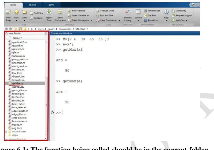
To call the function from the command window successfully, the function must be saved in the current folder that MATLAB read from as shown in figure 6.1.

Figure 6.1: The function being called should be in the current folder. Example 6.3

Write a function that receives two vectors and return the summation, dot product and subtraction of them and plot both vectors where first vector as a dependent variable and the second vector as independent variable.

Solution

Firstly we should specify how many inputs and outputs of the function, the function receives two vectors i.e. there are two inputs and returns summation, dot product and subtraction of the vectors i.e. three outputs, with regard to the plotting it does not consider an output because there is no numerical value returned form plotting

The code should be:

function [x,y,z] = getopr (a,b)

x = a+b;

y = a.*b;

z = a-b;

plot (a,b)

end

(53)

Function and Anonymous Function World Journal of Engineering Research and Technology

>> b=x.^2;

>> [m,n,o] = getopr(a,b)

The expression [m,n,o] was used to save the three outputs of the function in three variable and if we just call the function getopr(a,b), we should get only the first output and lose the others.

9.3 Sub function

For organizational purposes, user may have to call a function inside the main function in this case the main function which call another one is said to be primary function and the called function is said to be sub function.

For the example 6.3 you can write the code as follows

function [x,y,z] = getopr (a,b) % primary function

x = a+b;

y = a.*b;

z = a-b;

plotvec(a,b);

end

function [] = plotvec (n,m) % sub function

plot (n,m)

end

where the primary function getopr call sub function plotvec

9.4 Anonymous function Consider the following equation

If we would like to write it in MATLAB, we should tell it that x is a variable in the

equation y, to do that we can use the following expression: function name = @ (variables) [equation]

Example 6.4:

Find the value of the function

(54)

Solution

y= @(x) [x^3+x^2+3*x-10]; >> y(1)

ans = -5 >> y(5) ans = 155

Example 6.5:

Find the value of the function at the point (2,3)

Solution

In command window type the equation as follows z= @ (x,y) [x^2+y^2+x*y];

(55)

Plotting World Journal of Engineering Research and Technology

CHAPTER-10 PLOTTING 10.1 Introduction

MATLAB support plotting graphs and figures in two and three dimensional space. It supply tools that meet user’s needs.

10.2 plot command

plot function used to plot two quantities which is in general form:

plot(independent variable, dependent variable)

where independent quantity lies on x-axis (horizontal) and the dependent variable lies

on y-axis (vertical).

Example 1:

Let x=1:100; y = x.^2;

To draw the curve formed by x and y vectors you just use plot(x,y) the resulting drawing in the following figure

Example 10.1: if you have defined two vectors a = [1,2,3,4,5] ;

(56)

It is noticed that the drawing line is has fixed color and weight for all drawings.

10.2.1 Combination multiple graphs in one plotting window

MATLAB support plotting two or more graphs in one window by assigning each pair of quantities successively.

Example 10.2:

(57)

10.2.2 Definition drawing line properties

1- line color: MATLAB has basic colors shown its codes in the table below

Color Code

White w

Black k

Yellow y

Blow b

Red r

Green g

Cyan c

Magenta m

For the example 1 it can be change line color to red by the adding color code to plot function

(58)

Or yellow by:

plot(x,y,'y')

10.2.3 Line style specifiers

It can be set line style by assigning line specifier to plot function. Specifiers are listed in the table:

Specifier Line style

‘-’ Solid line (default) ‘--’ Dashed line ‘:’ Dotted line ‘-.’ Dash-dotted line

Return to example 3 and change plot command

(59)

10.2.4 Marker specifiers

The table below list makers specifiers that can be assigned to plot function so as to change the node syle.

Specifier Marker type

‘+’ Plus sign

‘o’ circle

‘*’ Asterisk

‘.’ Point

‘x’ Cross

‘square’ or ‘s’ Square ‘diamond’ or ‘d’ Diamond

‘^’ Upward-pointing triangle ‘>’ Right-pointing triangle ‘<’ Left-pointing triangle

'pentagram' or 'p' Five-pointed star (pentagram)

'hexagram' or 'h' Six-pointed star (hexagram)

Back to example 2 change plot command to:

plot (a,b,'s');

If you specify a marker, but not a line style, only the markers are plotted

(60)

Example 10.3:

x=1:30;

plot(x,sind(2*x),'-mo',...

'MarkerEdgeColor','k',... 'MarkerFaceColor','b',...

'MarkerSize',10)

10.2.5 Line width

Line weight or width can be changed by assigning 'LineWidth' property followed

by a number represent line width. Consider example 2 and change the plot command to : plot (a,b,'LineWidth',6);

(61)

Example 10.4:

x=1:30;

y=sind(20*x); z=cosd(30*x);

plot(x,y,'-ro',x,z,'k:s')

10.3 hold on command

This command enable overriding multiple plot commands to draw their graphs in a single drawing window

Example 10.5 :

x=1:30;

y=sind(20*x); z=cosd(30*x);

plot(x,y,'-mo',...

'LineWidth',2,...

hold on

plot(x,z,'-gs','LineWidth',3,...

(62)

10.4 Figure command

This command used to plot another graph in new window.

In example 6 you can separate the two graphs by insert figure command between the two plot commands:

clear; clc; x=1:30;

y=sind(20*x); z=cosd(30*x);

plot(x,y,'-mo',...

figure;

'MarkerEdgeColor','r',... 'MarkerFaceColor','b',...

(63)

10.5 adding labels, title and grid

By assigning xlabel, ylabel and title next to plot command you can add x label, y label and title respectively to the graph also to show the grid you have to use grid on command.

Example 10.6 Let

x =1:180; y = sin(x);

we do plot x and y by plot command

plot(x, y),

next we can add x label, y label and title to the graph

xlabel('x'),

ylabel('Sin(x)'),

title('Sin(x) Graph'),

to show the grid use grid on command

grid on,

% axis equal

10.6 adding legend

Sometimes it is helpful to add legends to the graph so as to define a specific graph type , so we have modified code in example 6 to show legends

clear; clc; x=1:30;

y=sind(20*x); z=cosd(30*x);

plot(x,y,'-mo',...

hold on

(64)

'MarkerFaceColor','b',...

'MarkerSize',8)

legend('sin (x)','cos (x)');

It is possible to choose where you put your legends on the graph by assign a string value for ‘Location’ property, for example:

legend('sin (x)','cos (x)','Location','northwest');

Table below shows several specifiers for Location property

Specifier Location in Axes

North Inside plot box near top South Inside bottom

East Inside right

West Inside left

NorthEast Inside top right (default for 2-D plots) NorthWest Inside top left

SouthEast Inside bottom right SouthWest Inside bottom left

NorthOutside Outside plot box near top SouthOutside Outside bottom

EastOutside Outside right WestOutside Outside left

NorthEastOutside Outside top right (default for 3-D plots) NorthWestOutside Outside top left

SouthEastOutside Outside bottom right SouthWestOutside Outside bottom left

(65)

10.7 Subplot command

Subplot enable users to separate plotting window to many sub-windows and draw a certain graph in a specific window.

The general formula is subplot(m,n,N)

Where m is number window row, n is number of window column and N is the number of the window that should appear the graph which plotted directly after calling subplot command. Example 10.7 clear; clc; x=1:30; y=sind(20*x); z=cosd(30*x); k=secd(20*x); r=cscd(30*x); subplot(2,2,1)

plot(x,y,'-mo',...

subplot(2,2,2)

'MarkerEdgeColor','r',... 'MarkerFaceColor','b',...

'MarkerSize',8)

subplot(2,2,3)

plot(x,k,'-gs','LineWidth',2,...

'MarkerEdgeColor','c',... 'MarkerFaceColor','r',...

(66)

subplot(2,2,4)

plot(x,r,'-gs','LineWidth',1,...

'MarkerEdgeColor','k',... 'MarkerFaceColor','m',...

'MarkerSize',5)

10.8 Specifying axes for legend

Create a figure with two subplots and return the two axes objects, ax1 and ax2. Plot random data in each subplot. Add a legend to the upper subplot by specifying ax1 as the first input argument to legend.

clear; clc;

y1 = rand(3);

ax1 = subplot(2,1,1); plot(y1)

y2 = rand(5);

ax2 = subplot(2,1,2); plot(y2)

(67)

10.9 Axis property

Sets the limits for the x- and y-axis of the current axes and has the general form : axis([xmin xmax ymin ymax])

where xmin, xmax, ymin and ymax are minimum limit on x-axis, maximum limit on x-axis, minimum limit on y-axis and maximum limit on y-axis respectively.

Example 10.8

x =1:180;

y = sin(0.3*x); plot(x, y), xlabel('x'),

(68)

10.10 Shape drawing

In this section we will focus on drawing different shapes in MATLAB which users may get use of them in solving some engineering problems.

10.10.1 Line object

The function line allow us to plot line object between two points, the general expression is:

line([x1,x2],[y1,y2])

where x1 is the x-coordinate of the first point

x2 is the x-coordinate of the second point y1 is the y-coordinate of the first point y2 is the y-coordinate of the second point

user can add as many properties as he wish to the line object like what we study previously

Example 10.9

Draw a line between the points (2,3) and (4,8) Solution

Let us use command window to call line function line ([2,4],[3,8])

(69)

Figure 10.1: Drawing Line object. 10.10.2 Rectangle object

The function rectangle in MATLAB is responsible for creating rectangle object with sharp or curved corner. The general expression is

1- Rectangle with sharp corner: rectangle(‘Position’, pos)

where ‘Position’ is a rectangle property which assign the position of the rectangle.

while pos is holding the values [x, y, w, h] where x is start point x-axis

y is start point y-axis w is width of the rectangle h is height of the rectangle

Example 10.10

Draw a rectangle its corner at the point (2,3) and has 5 width and 6 height Solution

Type in the command window rectangle('Position',[2 3 5 6]) >> axis([0 10 0 10])

>>

(70)

Figure 10.2: Creating rectangle with sharp corner. 2- Rectangle with curved edge :

rectangle('Position',[x,y,w,h],'Curvature',v)

where curvature is the rectangle property that assign curved shape to the rectangle corners and v is the value of the curvature.

Example 10.11

Draw a rectangle start from the point (2,3) and has 5 width, 6 height and 0.2 radius of the curvature of the corner.

Solution:

rectangle('Position',[2 3 5 6], 'curvature',0.2) >> axis equal

(71)

10.10.3 Circle object

Unfortunately there is no direct function to draw a circle that is defined by its radius coordinate and value, so we have to build our own function. We have known from algebra that the general form of a circle equation having (a,b) radius coordinate and (R) value shown in figure 10.4 is:

Figure 10.4: Circle scheme.

Where:

Thus, we wrote the code below after we had use the equations above % This code function is written by Hazim Nasir

% The function is plots a circle by receiving circle

radius and coordinate

function [] =drawCircle (radius,x_rad,y_rad)

r=radius;

k=0;

a=x_rad;

b=y_rad;

for theta=0:pi/200:2*pi

k=k+1;

(72)

end

x=x_init+a;

y=y_init+b;

plot(x,y)

grid on

end

The previous code considered that R vector has rotated from 0 to 2pi angle with a step of pi/200.

10.11 grid on command

By typing grid on command after plot function a grid will be activated in the plot window.

10.12 data cursor

Figure 10.5 illustrates data cursor icon, after left click on this icon, if the user clicking on a specific point at a graph MATLAB will return information about this clicked point involves its coordinates.

Figure 10.5: Circle scheme. 10.13 ezplot

Easy to use function, This plotter has used for drawing equations with a specific interval and come with many overloads:

1- ezplot(equ) : where equ is f(x) here MATLAB use the default domain .

(73)

3- ezplot(equ,[ Xmin Xmax Ymin Ymax ]): plots f(x) over the domain

and

4- ezplot(string): easy to use plotter accept any equation as a string. For example: ezplot('x^2')

ezplot('x^2-y^4')

5- ezplot(equ,[xymin,xymax]) plots equ(x,y) = 0 over the domain and

Example 10.12

Draw the following using easy to use function:

1.

2. where

3. over the domain

Solution:

ezplot(x^3+1)

ezplot(sin(x),[-pi,pi])

ezplot('x^2-y^4')

Figure 10.6 illustrates the drawings returned by the plotter

(74)

CHAPTER-11

SYMBOLIC COMPUTATIONS 11.1 Introduction

Most of the mathematical operations that the engineers and scientists make are symbolic representation of the quantities or equations or any other relational variables. One can perform different operations on these symbolic representations such as differentiation, integration or solving equations that may appear in design problems. This chapter introduce the symbolic variables definition and lead the way to the following chapters which are deal with very important operations like solving algebraic and differential equations and calculus operations

11.2 Symbolic object

In MATLAB users can use sym function to create symbolic object, for example you can create symbolic variables a and b as follows:

a = sym('a'); b = sym('b');

or you can use a shortcut to simply the above variable definition with syms command: syms a b

if you have y = f(x) you can write it down as syms y(x)

11.2.1 Assumptions

state can be assigned to the symbolic variable, state can be either real or positive for example if we assume that a is real and b is positive:

a = sym('a','real'); b = sym('b','positive');

These assumptions can be checked by the command assumptions

(75)

Symbolic Computations World Journal of Engineering Research and Technology

11.2.2 Number representation

sym function was used for representation technique for numbers by assigning second

argument which is either ‘r’, ‘f’, ‘d’ or ‘e’ where ‘r’ refer to rational for example:

If there is no exact rational number MATLAB will return expression of the form

y*2^x with very large integers x and y. ‘d’ refer to decimal

‘e’ stands for estimate error

‘f’ refer to "floating-point."

(76)

11.3 Symbolic matrices Use the general form:

matrix name = sym('variable', [matrix dimension]) to produce an array of symbolic variables, for example:

where %d refer to element index. Another example:

11.4 Finding symbolic variables in expression

To determine the symbolic variables forming an equation, symvar is used to do that symvar ‘equ’ where equ is the equation which is desired to determine its symbolic

variables for example if we would like to get the variables of the equation we should write:

(77)

Calculus World Journal of Engineering Research and Technology

CHAPTER-12 CALCULUS 12.1 Introduction

We will focus in chapter 12 on calculus main subjects differentiation, integration, vector analysis, series, limits and transforms.

12.2 Differentiation

Differentiation of a function or equation can be performed by the function diff( ) which has the following overrides:

1- diff (eqn): differentiate equation (eqn) with respect to variable determined by

synvar function see section (11.4) Example 12.1

Differentiate the equation :

Solution:

In this example diff function differentiate the function with respect to x which is the

default variable determined by symvar

2- diff(eqn,var): differentiate the equation (eqn) with respect to particular variable

(var).

Example 12.2

Differentiate the equation : with respect to the variable r

(78)

3- diff(eqn,var,n): differentiate equation (eqn) to the order (n)with respect to variable (var).

Example 12.3

Differentiate the equation in example 12.2 to the order 2 Solution:

12.3 Integration

MATLAB supports both definite and indefinite integrals by the function int ( ). For

indefinite integral use the general expression: int (expr, var )

where int function integrate the expression (expr) with respect to the variable (var). Example 12.4

Integrate the expression:

Solution:

For definite integral use the expression: int(expre, var ,a, b)

in this expression int function integrate the expression (expre) with respect to the variable (var) from a to b.

Example 12.5

(79)

Calculus World Journal of Engineering Research and Technology

Solution

Example 12.6

Integrate the symbolic matrix:

Solution:

12.3.1 IgnoreSpecialCases property

Assume you have this expression where both x and n are variables. Now if you

integrate this expression with respect to x variable int function will return the answer as a piecewise object ,which is the default option for int function, where each solution is correspond to a specific value or range of values of the equation parameters:

(80)

CHAPTER-13

SOLVING EQUATIONS AND SYSTEMS 13.1 Introduction

Solving equations subject will be covered in this chapter symbolically by using Symbolic Math Toolbox which is supports numeric and symbolic solving for the equations.

13.2 Equation definition

Equations are represent in MATAB by a set of symbolic variables, operators or numerical values on both sides of == operator. For example to represent the equation

we should write the following script: syms x y

sin(x)+3*x-y == 4

you may assign the equation to some variable: d = sin(x)+3*x-y == 4

13.3 Converting linear equations to matrix form

There is equationsToMatrix function to put a set of linear equations in the form of a matrix, the general expression for this function is :

[L,R] = equationsToMatrix([eq1,eq2,…eqn ], [variable])

Where eq1,eq2 are the linear equations desired to convert and n number of equations in the set, the second input argument is variable which is a vector contains a set of the

variables that are form the equations. The output argument L holds the coefficient matrix, the left side of the equations, and R is a vector holds the right side parameters of the equations.

In case of did not assign variable as a second input argument:

[L,R] = equationsToMatrix([eq1,eq2,…eqn, ]) MATLAB will use symvar command to get the symbolic variables in the equations

Example 13.1

(81)

Solving Equations and Systems World Journal of Engineering Research and Technology

Solution

syms x y z k

a1=3*x+2*y+z-2*k==0 ;

a2=x-0.5*y-2*z+k== -3.5 ;

a3=0.3*x+y+0.7*z-3*k== -14.2 ;

a4=2*x+y+4*z+k==32 ;

[A,b] = equationsToMatrix([a1,a2,a3,a4],[x y z k])

MATLAB will be returning A and b as follows

It is clear that (b) is a 4x1 sym vector which is mean that its elements are a rational numbers by default.

13.4 Solving set of linear equations

The function that we may use to solve a system of linear equations is linsolve( ) and

take the expression x = linsolve(A,b)

where A and b are the coefficient matrix and vector containing the right side values of the system respectively and x is a vector involves the magnitude of the variables in

(82)

13.5 solve function

The system of equations which can be written in form matrix or say structural array can be solved by using the following expression:

solve(equation 1, equation 2, ……, equation n)

Where n equal to the number of the equations in the structural array Example 11.3

Solve the following system :

Solution : syms x y z

S = solve(3*x + 2*y-z == 13, x + y+z == 7,...

2*x-0.5*y+3*z==5)

The results will be S =

x: [1x1 sym] y: [1x1 sym] z: [1x1 sym]

to display x,y and z values write: [S.x S.y S.z] , then MATLAB will return their values respectively :

ans = [ 2, 4, 1]

You can also use the multiple output argument to get all the solutions: [x y z] = solve(3*x + 2*y-z == 13, x + y+z == 7,...

(83)

13.6 Algebraic equation

The function solve can be used to solve algebraic equations, the general expression is: solve(equation, var)

where equation : is the required equation to be solved

var: is the independent variable that the equation should be

solved for.

The operator == should be used to assign the right side to the left side of the equation The left side should

Example 13.2

Solve the following equations

with respect to the variable (x). Solution:

syms a b c x

solve(a*x^2+b*x+c == 0,x)

the answer is ans =

-(b + (b^2 - 4*a*c)^(1/2))/(2*a) -(b - (b^2 - 4*a*c)^(1/2))/(2*a) syms x

solve(x^4 + 2 == 3*x^2 - 1,x)

the results are: ans =

((3^(1/2)*i)/2 + 3/2)^(1/2) (3/2 - (3^(1/2)*i)/2)^(1/2) -((3^(1/2)*i)/2 + 3/2)^(1/2) -(3/2 - (3^(1/2)*i)/2)^(1/2)

Example 13.3

Solve the equation:

Solution:

If the right side of the equation equal to zero you have not to use == operator syms x

(84)

and the result will be: ans =

1 (3^(1/2)*i)/2 - 1/2 - (3^(1/2)*i)/2 - 1/2

If solve function failed to get the exact symbolic solution, it will return the numeric one, for example:

13.7 Determining Poles

In control theory poles are plays a great role in finding system stability and MATLAB

provide poles ( ) function to determine this quantity in this expression: poles(func,var,interv)

where func is the symbolic expression, var is the variable of the expression and interv is the interval which is MATLAB used to look for poles. If we do not assign interval to poles function, the default interval will be used which is the entire complex plane.

Example 13.4

Find the poles of the system

Solution

(85)

13.8 Ordinary differential equations

MATLAB is supports solving ordinary differential equations via many built in functions which are dsolve, ODE23 and ODE45 function.

13.8.1 dsolve function

This function have the following forms:

1- dsolve (eqn(n))

Where eqn is an ordinary differential equation of order n and the derivative part annotated by diff(variable)

Example 13.5

Solve the differential equation: