USING STRONG INFERENCE TO FALSIFY DIFFERENTIAL
EQUATION MODELS OF SUGAR MAPLE HEIGHT GROWTH
Rolfe A Leary
1, Vivian Kvist Johannsen
21Consultant, Rolfe A Leary & Associates, 1382 W. Iowa Av., St. Paul, MN 55108 USA, Ph./FAX: 651-646-8732/330-7687 2Department Head, Forest and Landscape, Faculty of Life Sciences, University of Copenhagen, Hørsholm, Denmark
Abstract. Platt’s research strategy called ‘strong inference’ is often studied, but is difficult to apply. Here strong inference is applied in selecting differential equation models of sugar maple, Acer saccharum
M., height growth. Two model groups proposed by Zeide (1993; Zeide, B. 1993. Analysis of growth equations. For. Sci. 39(3):594-616.) are supplemented with two additional groups, 1) size decline and 2) second order differential equations, nearly exhausting the possible height growth models currently in the literature. A ‘crucial experiment’ was to fit a simultaneous system of equations to height age data collected from a cohort of trees felled years earlier for stem analysis. Models for cohort members are identical in right-hand-sides, have common parameters, but have tree-specific initial heights. Common parameters and tree-specific initial heights are estimated during fitting. Results, based on stem analysis data for a cohorts of from three to five sugar maple growing on 54 plots in the Lake States, showed that all cohort members were predicted by logarithm of time decline (LTD) models to have extremely similar initial heights (<0.01 m range), which contradicts experience and leads to their falsification. Three of four models in the time decline (TD) class predict a very small range in final heights, but a large range in initial heights (from 6.4 to 2.9m), hence can also be considered falsified. Size decline and second order models could not be falsified using the height age cohort data available.
Keywords:cohort dynamics, Lyapunov exponent, tree questioning, chaotic models
1
Introduction
Forest dynamics research has been plagued since its early days by an embarrassing riches of possible growth equations for representing stand and tree property time dynamics, but few criteria for deciding among the equa-tions. When computers were first used for mathemat-ical modelling, goodness of fit was a primary criterion (Grosenbaugh 1958, Furnival 1961). In more recent years other statistical properties of estimated models and their parameters have become most important.
Suggested here is an analysis procedure that could be a component of a wider process of evaluating growth models that addresses the problem Zeide (1993) high-lights when he quotes Dover (1988): ”If physics has its laws, biology has its variety” – or, one might say, ‘forest growth modellers have their equations’. Well, variety is desirable if variety is needed and beneficial. But, forest dynamics research as a scientific discipline would bene-fit from fewer and truer growth equations, rather than more variety. A critical problem has been the general lack of tests to quickly classify equations into those that
warrant further investigation and those that do not, or those that may turn out to be ‘true’, from those that are definitely false. Missing from the process of equa-tion selecequa-tion has been the knowledge and experience of field silviculturalists and ecologists – equation evaluation has in recent years become almost solely a biometrical exercise.
Popper (1959) argued that scientists should attempt to falsify their hypotheses, rather than to confirm them – his recommended solution to the problem of induction. Hypotheses that survive repeated genuine attempts at falsification can then be taken as more believable than others that have not survived such attempts. Popper’s suggestion involves switching from the logical argument form typically used in inductive science, calledmodus po-nens (below left), but is invalid because it commits the error of affirming the antecedent, to modus tollens (be-low right). Modus tollens is a logically valid conditional argument form. It is understood that “A” in both cases consists of the scientific hypothesis, required assump-tions, and some initial conditions on important
vari-Copyright c2010 Publisher of the International Journal ofMathematical and Computational Forestry & Natural-Resource Sciences
ables. “B” in the first premise designates what should follow if the hypothesis, auxiliary assumptions, and ini-tial conditions are all true. The second premise, ‘B’ or ‘not B’ comes from field experiments.
If A then B B
therefore A
If A then B not B
therefore not A
In a widely cited paper, Platt (1964) made the case that some scientific disciplines are moving ahead faster than others. By examining the fastest moving scientific disciplines Platt was able to identify several important traits, which he refined and presented in his widely ac-claimed paper ‘Strong Inference’ (Platt 1964). He states: “Strong inference consists of applying the following steps to every problem in science, formally and explicitly and regularly:
1. devising alternative hypotheses
2. devising crucial experiments (or several of them), with alternative possible outcomes, each of which,
as nearly as possible, exclude one or more of the hypotheses,
3. carrying out the experiment so as to get a clean result, and
(1’) recycling the procedure, making sub-hypotheses or sequential hypotheses to refine the possibilities that re-main; and so on” (Platt 1964, italics in original).
Platt’s paper popularised the concept of forming more than one testable hypothesis that had been introduced much earlier (Chamberlin 1897). Platt’s several contri-butions included the use of exhaustive hypothesis forma-tion, combining exhaustive alternative hypothesis for-mation with tree questioning, and falsification using con-clusive experiments (McRoberts 1989).
As forest scientists we should be able to quickly iden-tify equations not worthy of further study for specific purposes. One consequence of our not having done so is what we have been experiencing – a kind of ’willy-nilly’ introduction of new growth equations and a prolonged ‘running in place’. Our ‘running in place’ has followed the generally inconclusive nature of model selection cri-teria based on goodness of fit of model to data, as well as its more recent variants.
If we had tough evaluation criteria, or a tough strat-egy, then models that do not fail a battery of tests based on sound criteria, and at the same time meet or exceed the best performance levels of models currently in use, could be further scrutinised for physical, biological or ecological interpretation of parameters, thus making at
least a small step from description toward explanation (Bossel 1991, Leary 1985).
Here we report an attempt to follow Platt’s rules quoted above for several forest growth models applied to the problem of modelling height growth. We begin with the problem of devising alternative hypotheses that ex-haust the range of possibilities, and then outline a ‘cru-cial experiment’ that can be conducted to eliminate one or more of the branches of hypotheses. Finally, we apply the process to growth equations proposed for modelling sugar maple tree height in the Lake States, USA, so as to get a ‘clean result’ and conclude by applying amodus tollens argument form to the findings.
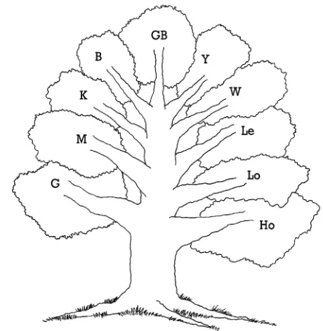
Figure 1: The ‘tree’ of growth equations suggested by forest scientists to about 1959, following Hossfeld’s model introduced in 1825, as assembled by Kiviste (1988) and Zeide (1993). Symbols are the first char-acter of model names in Table 1, with oldest models are at the bottom.
Step 1:
Form alternative hypotheses
that exhaust all possibilities
Table 1: Equations analysed by Zeide (1993) summarised in their differential form and the logarithm of their differential form as re-expressed by Zeide. In our case hdesignates total tree height,h designates one year height growth, t denotes total age, and A,B,C denote numerical constants. Parameters p and q are combinations of parameters required for the re-expression.
Equation name Differential form Logarithm of differential form Hossfeld IV h = h2A B t(−B−1) ln(h) = k + 2 ln(h) + qln(t) Gompertz h = h A B e(−B t) ln(h) = k + ln(h) + q t Logistic h=h(B−(B/A)h) ln(h) = k + 2 ln(h) + q t
Monomolecular h=B(A−h) ln(h) = k + q t
Levakovic I h=h A Bt(AC+tC) ln(h) = k + pln(h) + qln(t)
Korf h =h A B t(−B−1) ln(h) = k + ln(h) + qln(t)
Weibull h = (1−h)A B t(B−1) ln(h) = k + pln(t) + q t(p+1) Yoshida I h = (h−B)t(AA+tC) ln(h) = k + 2 ln(h−C) + qln(t)
Bertalanffy h=A h23 −B h ln(h) = k + 23 ln(h) + q t Generalized Bertalanffy h=A hC−B h ln(h) = k +pln(h) + q t
Table 2: Additional growth equations tested in this paper. h designates height growth,k designates acceleration of height, t denotes total tree age, and A,B,C denote model parameters.
Equation name Differential form Source and/or applications
Leary h=A h e−B h Leary (1970)
Zeide h=A hCe−B h Zeide (1993)
Schnute h =h k
k=k(A+B k) Schnute (1981), Bradenkamp and Gregoire (1988)
Schnute/Zeide h =h k
k=k(A kB) Zeide (1993)
Umemura/Hamlin hk ==Ck −A k−B h Umemura (1984), Hamlin (1987), Hamlin and Leary (1987)
in Figure 1.
Zeide argued that the rather simple equations he anal-ysed represent ’processes’, but ecological ones rather than physiological. The ’processes’ he identified are those of ’expansion’ by trees to fill available space and capture resources, and of ’decline’ in growth that occurs because of restraints imposed by ’environmental resis-tance’ and ageing, both of which are poorly understood ecological processes. By taking the logarithms of the dif-ferential equations, two categories of growth equations based primarily on the mathematical relation in the de-cline portion were identified. By a judicious combination of variables, Zeide isolated two basic forms for growth equations that included all except the Weibull equation:
lny=k+plny+qlnt, (1)
and
lny =k+plny+qt (2)
The growth equations, expressed as differential equa-tions, and also as the logarithm of the differential form are assembled in Table 1. Sloboda’s equation is omitted here because of its immense complexity.
Equations having the form of equation (1) were la-belled – LTD (for logarithm of time decline) and include: Hossfeld IV, Levakovic I (Levakovic III is omitted), Korf, and Yoshida I. Equations having the form of equation (2), were labelled – TD (for time decline). These in-clude Gompertz, logistic, monomolecular, Bertalanffy, and generalised Bertalanffy. The parameterization of the Weibull equation used by Zeide does not belong in either class because both its ’expansion’ and ’decline’ terms are based solely on time which would seem to cast doubt on its suitability as a biological growth model. The monomolecular equation is also suspect as a growth equation because it’s increase component is a constant not related to age or size.
hy-potheses exhaust all possible models. Here Zeide’s anal-ysis is a bit limiting because:
1. he initially limits his analysis to growth differential equations that have closed form (integral) solutions (Shvets and Zeide 1996),
2. he introduces the growth equation of Schnute that is formed as a second order differential equation, proposes a modification and does a preliminary test, but omits discussion of a another second order equa-tion introduced by Umemera (1984) and used by Hamlin (1987) and Hamlin and Leary (1987), and does not form a class of second-order equations,
3. he does not address the issue of different parameter-izations that are possible for some differential equa-tions that might affect their placement in a branch of the question tree, and
4. he rediscovers a new form of first order differential equation (Leary 1970), and adds a key parameter. The latter equation forms a new category of equa-tions in his schema because its decline is not de-termined by time or its logarithm, rather by size. Expressed in logarithms following Zeide’s notation it has a SD form, i.e.:
lny =k+plny+qy (3)
Tests reported here include the growth equations given in Table 1, plus the models formed as differential equations (Table 2).
Both the Leary and Zeide equations have closed form solutions, but they involve the exponential integral and are generally only accessible using methods from ad-vanced mathematics. To treat all equations with the same methods and software, we treated the first order differential equations as first order forward difference equations and fit them directly to the size – age data, using numerical solution methods to solve the equations as needed.
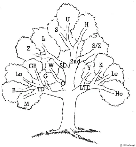
The collection of growth equations provided by Kiviste, and the analysis by Zeide showing there are essentially two major groupings of equations (TD and LTD), and a new classes (SD), provided us with the ini-tial spark of hope that a test based on strong inference principles might be possible. The addition of a fourth class based on second order models rounds out the four branches for tree questioning (Figure 2).
In sum, the four alternative hypotheses that appear to exhaust the possiblities are:
1. logarithm of time decline models (LTD) (Hossfeld IV, Levakovic I, Korf, Yoshida I)
Figure 2: Model classes after adding categories for size decline (SD) and second order (2nd) models to those
proposed by Zeide (1993), giving four main branches for ‘tree’ questioning. The ‘O’ for other/odd branch con-tains only one equation – “W” for Weibull.
2. time decline models (TD) (Gompertz, logistic, gen-eralized Bertalanffy, monomolecular)
3. size decline models (SD) (Leary, Zeide)
4. higher order models (2nd order) (Schnute,
Schnute/Zeide, Umemura/Hamlin).
Step 2:
Perform one or more crucial
experiments
The suggested steps in carrying out crucial experi-ments are four:
1. select a property of trees that covers a wide range of observed relative growth rates (e.g., stem analysis height – age data).
2. fit the differential equations directly to the selected tree size – age observational data so that all equa-tions, whether integrable in closed form or not, are treated with the same methods.
heights for one tree, has tree-specific initial condi-tion estimates, but the system has a common set of model parameter estimates.
4. supplement the traditional model selection criteria with an evaluation of the sensitivity of model pre-dictions at later ages to the estimated initial con-ditions at the initial time – here taken to be age 1 year.
Each step is discussed in more detail below.
1. Select a size property that changes as much as possible. One could argue that the property of tree height is more difficult to model than tree diameter or basal area because the model must initially predict very small values (fractions of meters) and then in-crease rapidly for some species, or slowly for others, to fairly large values (tens of meters). Fluctuations in cli-matic conditions can add interesting divots to these ba-sic patterns, making height growth relationships much more challenging than is often presented (e.g., Spurr 1952). The range of relative growth rates for height, es-pecially of naturally regenerating species, probably ex-ceeds that for diameter or basal area, although height relative growth rates may not have the range of rela-tive growth rates for biomass – from seed to mature tree. Contrasting height with, say, diameter or basal area measurements, tree heights exist from seed germi-nation, but, following convention, diameter and basal area are not measured until after trees reach 1.3m. Fur-ther reducing the utility of stem thickness at 1.3m is the usual practice of delaying tree diameter measurements until an age when trees are merchantable. Trying to fal-sify models of, say, breast height diameter or basal area growth of merchantable trees, is problematic because, speaking metaphorically, the data make few demands on the model, so many models can meet those reduced demands.
It is thus hypothesised that several models are more likely to perform indistinguishably well in that more lim-ited range of relative growth rates typically offered by tree diameter and basal area of merchantable trees. Be-cause of the stronger demands made on mathematical models, the first step in a crucial experiment of candi-date growth differential equations should be to obtain a complete set of height-age data, preferably from detailed stem analysis.
2. Fit the differential equations directly to size-age data. As noted above, we expand Zeide’s original 2 branch tree of alternative models to 4 branches. Equa-tions in branch 3 have no closed form solution using simple functions, hence if they are to be tested they
must be fit directly to the observational data – typi-cally in the<size-age>format. By fitting the equations in all branches directly to observational data, all four branches of hypotheses can be treated in the same way, including, for example, use of the same fitting and anal-ysis software. To mix up methods of estimating model parameters between those for fitting algebraic and dif-ferential/difference equations is to run the risk of not having a ’clean’ result.
3. Fit a system of differential/difference equa-tions to height-age data for a cohort of trees.
Rennolls (1995) argued the choice in height growth mod-elling is between modmod-elling mean tree height or individ-ual tree height. We suggest there is another option – to represent height growth of a cohort of trees. Because the trees selected are of the same species and have grown in close physical proximity, they should have experienced very similar growing conditions. Hence, their growth should be governed by the same model equations that have common parameters, but possibly slightly different initial conditions. For example we would fit the follow-ing equations to data collected from a 3-tree cohort felled for stem analysis:
h1 = A h1eB h1, h
1(t= 1) = k1
h2 = A h2eB h2, h
2(t= 1) = k2 (4)
h3 = A h3eB h3, h
3(t= 1) = k3 where h‘
1, h2, and h3 designate annual growth in total height of dominant trees, k1, k2, and k3 designate es-timated initial heights of the three trees, and Aand B denote estimated parameters common to all equations. Parameters are estimated by minimising a loss function based on squared deviations between predicted and ob-served heights.
As forest trees become more valuable, sacrificing cen-tral stems of dominant trees for age determination at, say, one meter intervals will probably become uncom-mon. Perhaps even less common will be the collection of stem analysis data on several trees growing in close proximity. However, when such data are collected, the felled trees will typically be all of the same social class and because they have grown in close proximity they will have experienced nearly identical growing conditions in both space and time, and can be represented using iden-tical model structure with common parameters.
Step 3: Conduct an experiment to get
a clean result
A) B)
C) D)
of experiments when comparing model performance for predicting breast height diameter or basal area in mer-chantable trees. We also argue that we need new tools for assessing the performance of growth equations in ac-counting for pattern in observational data. For exam-ple, Zeide (1993) compared model classes based on stan-dard error of estimated Norway spruce height, diameter, and volume derived from data published by Guttenberg (1915) and found several model classes were indistin-guishable as judged by the standard error of estimates, thus falling short of Platt’s imperative to ‘carry out the experiment so as to get a clean result.’
Introduced here is the dimension of sensitivity of model predictions to small changes in initial conditions. This criterion has special importance when structuring the test using stem analysis data on height growth of cohorts. A simple ratio of the differences between es-timates of, e.g., k1, k2, k3 (above), and the difference between predicted heights at a later age provides an ap-proximation to the Lyapunov exponent for system tra-jectories (Wolf, et al., 1985). Simply stated, if the Lya-punov exponent for a simultaneous equation model ap-plied to a particular species is positive, trajectories are diverging (differences in predicted heights of individual trees are becoming larger with time), if the exponent is negative trajectories are converging (differences in pre-dicted heights of individual trees are becoming less as the trees age), and if the Lyapunov exponent is zero, or nearly so, the trajectories are parallel or nearly so (dif-ferences in initial heights are predicted to be preserved through the life of the stand). This criterion was unex-pectedly decisive in choosing among the different model forms we tested.
2
Material
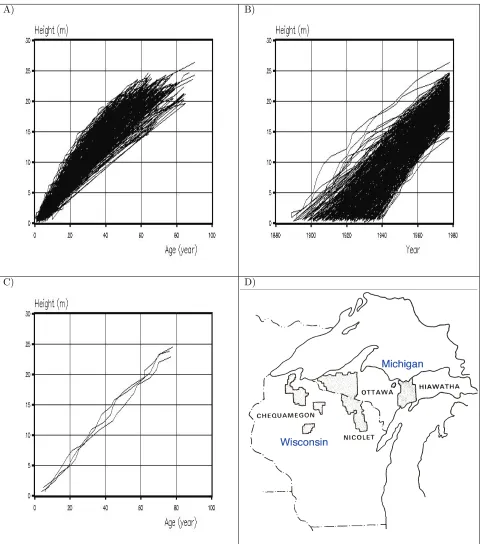
Stem analysis <height – age> data was available for cohorts of sugar maple (Acer saccharumM.) trees grow-ing in Wisconsin and Upper Michigan. These stem anal-ysis data had been collected for a large study of north-ern hardwood site productivity (Carmean 1978). Figure 3 shows height – age data for 54 plots located on the Chequamegon (21), Nicolet (11), and Hiawatha (22) Na-tional Forests in Wisconsin and Upper Michigan, USA. Figure 3A shows data in a typical height – age relation, 3B shows data in height – Julian date format, 3C shows a typical cohort of trees indicating that the observed range in final heights is typically about 2 m, and 3D shows the study plot locations. In selecting plots for in-clusion in the study, plots had to have from 3 to 5 sugar maple trees at least 45 years of age that showed they all regenerated within a 5 year period. Fifty four plots met these criteria.
3
Methods
Standard methods were used to collect field data and perform ring counts on discs removed at four foot incre-ments up the stem (Carmean 1978). To fit the system of difference equations we wrote a SAS program to im-plement a shooting method of fitting first order forward difference equations directly to size – age observations (Johannsen 2002).
The method for representing trajectory patterns for a cohort (produced by solving the simultaneous system of growth equations, subject to estimated tree-specific initial conditions and common parameters) was to form a single number as follows: divide the range in projected heights at an ‘advanced’ age (in our case 60 years) by the largest range of estimated initial heights among the three to five trees. A ratio could also be formed based on the smallest differences, but using the largest difference forms a somewhat less tough test. If the model predicts that the difference between tree trajectories is expand-ing, the ratio is greater than 1.0, if convergexpand-ing, less than 1.0, and if trajectories are parallel, the ratio is near 1.0. These values translate into positive, negative, and zero (respectively) Lyapunov exponents, that in turn suggest that height growth of the cohort is chaotic (diverging), or non-chaotic (converging or parallel trajectories).
4
Results
A cohort trajectory analysis was a very effective test for the strong inference method. Rather than estimate the true Lyapunov exponent, to measure divergence, convergence or parallelness of cohort height trajectories we expressed the pattern as a ratio of the range (max -min) of predicted heights at age one year and the range of predicted heights at harvest age – standardised to 60 years. Ratios for all equations are given in Table 3, based on the estimations for all combinations of plots and equations. In a few cases the estimation method did not converge for specific plots. Those plots are omitted from the summary.
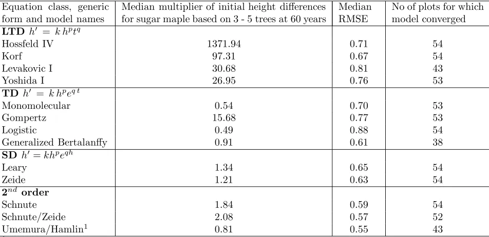
Table 3: Summary of trajectory analysis of growth equations based on fitting to height – age stem analysis data for a cohort of sugar maple trees on 54 plots. ‘Multipliers’ are determined by dividing the predicted range in final heights at 60 years, by the estimated range in initial heights.
Equation class, generic form and model names
Median multiplier of initial height differences for sugar maple based on 3 - 5 trees at 60 years
Median RMSE
No of plots for which model converged
LTD h = k hptq
Hossfeld IV 1371.94 0.71 54
Korf 97.31 0.67 54
Levakovic I 30.68 0.81 43
Yoshida I 26.95 0.76 53
TD h = k hpeq t
Monomolecular 0.54 0.70 53
Gompertz 15.68 0.77 53
Logistic 0.49 0.88 54
Generalized Bertalanffy 0.91 0.61 38
SD h=khpeqh
Leary 1.34 0.65 54
Zeide 1.21 0.63 54
2nd order
Schnute 1.84 0.59 54
Schnute/Zeide 2.08 0.57 52
Umemura/Hamlin1 0.81 0.55 43
1We used the ‘natural’ boundary condition (h(0) == 0), so all initial conditions were identical. The Lyapunov exponent
approximations are based on heights att= 1.
in cohort heights at age 1 is (2m/27) = 74.1mm. We concluded that LTD models exhibit diverging trajecto-ries, which translates into extreme sensitivity to initial conditions.
In contrast to multipliers for LTD models those mod-els in the TD class had multipliers less than 1, with the exception of the Gompertz equation (Table 3, column 2). Multipliers less than 1 indicate height growth trajecto-ries of cohort members are converging. If they are in fact converging, from what initial heights are they con-verging? Again we use the observation of a 2m range in heights of cohort members at age 60, and ask, if trajec-tories are converging to ‘pass through’ the 2m window at age 60, what was the range in cohort heights at age 1? The median multipliers for monomolecular, Gompertz, logistic, and Generalized Bertalanffy were 0.54, 15.68, 0.49, and 0.91 respectively. These ratios translate into initial height ranges of 3.7m, 0.128m, 4.08m, and 2.20m, respectively.
5
Discussion
We can conclude the following:
1. The class of models called logarithm-of-time-decline (LTD) (Zeide 1993) failed the trajectory behaviour test because they claim tree cohorts at maturity
have practically identical initial heights (less than 1 cm range). [Note: The test results are not critical to the initial year. We could as well have chosen 2 or 3 years of age.]
2. At issue in the trajectory behaviour test is the ques-tion of the height distribuques-tion in 1 year old seedling stands that will produce the cohort of trees at ma-turity. All areas of an aged forest will, even-tually, have a cohort of mature trees. If we know the range of heights at maturity, we can use the concept of a Lypunov exponent to work backwards to the range in heights of regenerated trees. How similar must these 1 year old seedlings be in total height to not exceed the observed range of cohort members at maturity; 1 m, 1 cm, 1 mm?
Table 4: AModus tollens conditional argument.
if ⎡ ⎢ ⎢ ⎣
LT Dmodelsare true and observed final heights are true
and auxillary assumptions are true
⎤ ⎥ ⎥ ⎦ then
⎡ ⎢ ⎢ ⎣
predicted range in initial heights of1year old seedlings that
will be in a final cohort <0.00?m
⎤ ⎥ ⎥ ⎦ ⎡
⎣ atobserved range in heights1year of age of all potential cohort members > 0.??m
⎤ ⎦
——————————————————–
T herefore
LT Dmodels are false
Figure 4: Idealised completion of the first cycle of a strong inference – based evaluation of height growth models based on extreme sensitivity to initial conditions.
When LTD models as a group give positive Lyapunov exponents (mulitpliers much greater than 1.0), it implies that the cohort system is chaotic with respect to height development. Because the experience of field foresters and ecologists seems to be that height development of a cohort of sugar maple trees is not chaotic, we conclude the LTD class of models is false by following a modus tollens conditional argument presented on Table (4).
If field sampling shows that the range in heights of year-one regenerated trees is one or two orders of mag-nitude greater than LTD models predict, we conclude that all LTD models are false, which will complete the first cycle in the strong inference process (Figure 4).
A second cycle of the strong inference process is to select another still-attached branch of models (Figure 4) and devise a crucial experiment to falsify all of its mem-bers.
Time-decline (TD) models can be further tested for their tendency to predict nearly identical final heights, and, for some, widely different, or in one case, negative, initial heights. From Figure 3C we saw that the range of final heights of one cohort is about 2m. Using the mul-tipliers for TD models in Table 3, we can divide 2m by the multiplier to estimate the range of first year heights. For the 54 plots of sugar maple used here, the ranges in first year heights are: monomolecular (4.66m), Gom-pertz (0.10m), logistic (6.38m), and generalized Berta-lanffy (2.85m). Again, field sampling should be under-taken, but it seems highly unlikely that the range in heights at year one is more than 1m. Recall, the arbiter is range in initial heights, not height itself. So, if we un-dertook a second iteration of the strong inference strat-egy as just described, we would have failed the conclusive experiment step – because the Gompertz is not falsified. However, all other models in the TD branch appear to be falsified (Figure 5). As noted, the monomolecular equation also predicts negative initial heights.
Figure 5: Idealised execution of the second iteration of a strong inference strategy based on the large range in ini-tial heights predicted by TD equations. The Gompertz equation is not falsified.
early growth and cohort trajectory behaviour. There are several remaining causes for concern: a) the effect different model parameterizations might have on the results of this analysis. We have used the parameterizations in Zeide (1993).
b) there have been more recent efforts to synthe-size growth equations (Garcia 2005) which were not in-cluded,
c) this report focuses on representing height growth patterns for cohorts of (Acer saccharumM.) growing the Lake States region of the United States in the general period 1890 to 1970. Our conclusions must be limited to this species growing in this period.
6
Conclusion
Using the four steps proposed in the method of ‘strong inference’ we have used stem analysis data collected on cohorts of 3 to 5 sugar maple trees from 54 plots to falsify all models Zeide calls logarithm of time-decline (LTD) (Hossfeld IV, Korf, Levakovic I, Yoshida I) because of their extreme sensitivity to initial conditions. There seems to be evidence that several members of the time-decline (TD) class can also be falsified (monomolecular, logistic, generalized Bertalanffy) based on their predic-tions of a wide range of initial heights but very similar final heights. There remains the task of falsifying the Gompertz model, the two models in the size decline class
(SD), and three models in the 2ndorder class.
Acknowledgements
Portions of this work were undertaken while the se-nior author was employed by the Danish Forest and Landscape Research Institute, Hørsholm, Denmark, and USDA Forest Service, North Central Forest Experiment Station, St. Paul, Minnesota. We thank J. P. Skovs-gaard and A. Robinson for support and useful discus-sions, and A. Pasvogel for illustrations. We also thank 3 anonymous reviewers for helpful comments.
Literature Cited
Bossell, H. 1991. Modelling forest dynamics: moving from description to explanation. For. Ecol. and Manage. 42:129-142.
Bradenkamp, B. and T. Gregoire. 1988. A forestry ap-plication of Schnute’s generalized growth function. For. Sci. 34(3):790-797.
Carmean, W.C. 1978. Site index curves for northern hardwoods in northern Wisconsin and Upper Michi-gan. USDA For. Serv. Res. Pap. NC-GTR-160. 16 p.
Chamberlin, T.C. 1897. Studies for Students: The method of multiple working hypotheses. Jour. of Geol. V(VIII):837-848.
Dover, G. 1988. RDNA world falling to pieces. Nature 336:623-624. (Cited from Zeide 1993)
Furnival, G. 1961. An index for comparing equa-tions used in constructing volume tables. For. Sci. 7(4):337-341
Garcia, O. 2005. Unifying sigmoid univariate growth equations. FBMIS Volume 1, 2005, 63 –68.
Grosenbaugh, L.R. 1958. The elusive formula of best fit: A comprehensive new machine program. USDA For. Serv. Res. Pap. SO-OP-158. 9 p.
Guttenberg, A.R. von 1915. Growth and yield of spruce in Hochgebirge. Franz Deuticke, Wien. 153 p. [In German] [Cited from Zeide, 1993]
Hamlin, D. 1987. A differential equation model of tree growth and its application in the study of forest site quality. Ph.D dissertation, University of Minnesota, St. Paul. 163 p.
Johannsen, V.K. 2002: Documentation for data analy-sis of Norway spruce, Dynamic Growth Models for Danish Forest Tree Species, Working Paper No. 19. Forest and Landscape, Denmark. 113 pp.
Kiviste, A.K. 1988. Mathematical functions of for-est growth. Estonian Agricultural Academy, Tartu. 108 p. + Supplement 171 p. (Cited from Zeide 1993)
Leary, R. 1970. System identification principles in studies of forest dynamics. USDA For. Serv. Res. Pap. NC-RP-45. 38 p.
Leary, R. 1985. A framework for assessing and reward-ing a scientist’s research productivity. Scientomet-rics 7(1-2): 29-38.
McRoberts, R. 1989. A survey of research strategies. P. 25-31in Discovering New Knowledge About Trees and Forests. R. Leary, compiler. USDA Forest Ser-vice RP-NC-135. 114 p.
Platt, J. 1964. Strong inference. Science 146:347-353.
Popper, K. 1959. The logic of scientific discovery. Harper & Row, New York. 480 p.
Rennolls, K. 1995. Forest height growth modelling. For. Ecol. Manage. 71:217-225.
Schnute, J. 1981. A versatile growth model with statis-tically stable parameters. Can. J. Fish. Acquatic Sci. 38:1128-1140.
Shvets, V. and B. Zeide. 1996. Investigating param-eters of growth equations. Can. J. For. Res. 26:1980-1990.
Spurr, S. 1952. Forest inventory. Ronald Press, New York. 476 p.
Umemera, T. 1984. An entirely new growth curves based on a second order linear differential equation. P. 591-597inIUFRO symposium on forest manage-ment and managerial economics. Tokyo, Japan.
Wolf, A., J.B. Swift, H.L. Swinny, and J.A Vastano. 1985. Determining Lyapunov exponents from a time series. Physica 16D(1985):285-317.