Application of computational intelligence methods
for the automated identification of paper-ink samples
based on LIBS
Krzysztof Rzecki1 , Tomasz So´snicki1 , Mateusz Baran1 , Michał Nied´zwiecki1 ,
Małgorzata Król2, Tomasz Łojewski3, U Rajendra Acharya4,5,6 , Özal Yildirim7 , and Paweł
Pławiak1*
1 Faculty of Physics, Mathematics and Computer Science, Cracow University of Technology, Warszawska 24,
31-155 Krakow, Poland; [email protected] (K.Rz.); [email protected] (T.S.); [email protected] (P.P.); [email protected] (M.B.); [email protected] (M.N.)
2 Laboratory for Forensic Chemistry, Faculty of Chemistry, Jagiellonian University, Ingardena 3, 30-060
Krakow, Poland; [email protected] (M.K.)
3 Faculty of Materials Science and Ceramics, AGH University of Science and Technology, Mickiewicza 30 Av.,
Krakow 30-059, Poland; [email protected] (T.Ł.)
4 Department of Electronics and Computer Engineering, Ngee Ann Polytechnic, Singapore;
[email protected] (R.A.)
5 Department of Biomedical Engineering, School of Science and Technology, Singapore School of Social
Sciences, Singapore; [email protected] (R.A.)
6 School of Medicine, Faculty of Health and Medical Sciences, Taylor’s University, 47500 Subang Jaya,
Malaysia; [email protected] (R.A.)
7 Department of Computer Engineering, Munzur University, Tunceli, Turkey; [email protected] (O.Y.)
1
2
3
4
5
6
7
8
9
10
11
12
13
14
15
16
* Correspondence:[email protected](P.P.),[email protected](K.Rz.)
Abstract:Laser-inducedbreakdownspectroscopy(LIBS)isanimportantanalysistechniquewith
applicationsinmanyindustrialbranchesandfieldsofscientificresearch.Nowadays,theadvantages of LIBSareimpaired bythemaindrawbackin theanalysisof collecteddata. Thisprocedureis essentiallybasedonthecomparisonoflinespresentinthespectrumwithaliteraturedatabase.This paperproposestheuseofvariouscomputationalintelligencemethodstodevelop areliableand fastclassificationofnon-destructivelyacquiredLIBSspectraintoasetofpredefinedcl asses.We focusonaspecificproblemofclassificationofpaper-inksamplesinto30separate,predefinedclasses. Foreachof30classes(10pensof eachof 5inktypes combinedwith10sheetsof 5paper types plusemptypages)100LIBSspectraarecollected. Fourvariantsofpreprocessing,sevenclassifiers (Decisiontrees,Randomforest,k-NearestNeighbour,SupportVectorMachine,ProbabilisticNeural Network,Multi-LayerPerceptron,andGeneralizedRegressionNeuralNetwork),5-foldstratified cross-validationandtestonanindependentset(formethodsevaluation)scenariosareemployed. Ourdevelopedsystemyieldedanaccuracyof99.08%withaverageclassificationtimeofabout0.12s isobtainedusingtherandomforestclassifier.Ourresultsclearlydemonstratesthatmachinelearning methodscanbeusedtoidentifythepaper-inksamplesbasedonLIBSreliablyatafasterrate.
Keywords:classification;computationalintelligencemethods;discriminationpower;LIBS;machine
learning;paper-inkanalysis 17
1. Introduction
18
During the decade, there have been important developments in laser induced breakdown 19
spectroscopy (LIBS). This atomic emission spectroscopy technique, also known as laser induced plasma 20
spectroscopy (LIPS), is used for qualitative and quantitative chemical analysis of samples in all states of 21
matter [1]. In this technique, high-power, short-duration laser pulse causes an ablation of the analyzed 22
material, which due to its high temperature (10 000K) dissociates into excited ions and atoms. When 23
plasma cloud cools down this excited species revert to lower energy states and emit optical radiation 24
which could be recorded and analyzed, revealing information about the elemental composition of 25
the sample [2]. LIBS spectra are generally very rich in emission lines coming from excited atoms and 26
ions occuring in a high temperature plasma cloud. Physical and chemical phenomena behind LIBS 27
are not fully understood yet, as they are very complex in nature. Nevertheless, LIBS applications 28
are recently rapidly growing due to the number of advantages of this method. The most important 29
ones are minimally destructive measurement with little or no sample preparation, efficiency and 30
possibility to analyze in real-time all elements in a single laser shot in all three states [3]. For solids both 31
mapping (2D) and depth profiling (3D) can be obtained. LIBS can be used for quantitative chemical 32
analysis, material identification and discrimination. This method can be applied in the laboratories and 33
industrial plants, and even at stand-off distances of tens of meters [4]. These properties predispose the 34
LIBS technique for use in many fields: space exploration [5], remote analysis of hazardous materials [6], 35
on-line quality control in various industries [7], cultural heritage studies [8], forensic chemistry [9,10], 36
geology [11], weld quality assurance [12], robotics [13] and many others [14–17]. 37
Although currently LIBS is already an established technology, spectrochemical LIBS analysis is 38
not straightforward. Identification of elemental constituents in the sample is usually based on the 39
strongest lines present in the LIBS spectrum (so called persistent lines), which are compared with a 40
literature database collected for all the elements from the periodic table. This analysis is cumbersome 41
and time-consuming because the emission spectrum is determined also by the properties of the plasma, 42
not only by the composition of the examined sample [18]. 43
At present, the great advantages of LIBS seem to be impaired to some extent by the main 44
drawbacks: problems coming from often poor signal reproducibility, the impact of sample composition 45
on signals recorded for individual components (matrix effects) and the difficulty of performing an 46
overall reliable data analysis (sometimes over 500 spectral lines need to be interpreted). Thus, a 47
question immediately raises whether the LIBS method can be supported by the modern achievements 48
in the field of computational intelligence [19] in an attempt to overcome the limitations of the current 49
LIBS spectrum analysis methodology. The analogous problem of classification of one dimensional 50
series of data is well known in computer science. The methods developed for this problem have been 51
successfully applied in many areas [20–27]. So, application of machine learning methods to LIBS 52
spectra of samples may certainly give a strong impact for further developments and applications. 53
Motivated by the aforementioned arguments we decided to apply computational intelligence 54
methods to the classification of paper-ink samples for forensic purposes, based on LIBS spectra of the 55
samples. The problem of discrimination of different paper-ink samples has already been addressed 56
in previous studies based on the LIBS spectrum analysis. Trejos et al. showed [28] that the highest 57
discrimination power (DP) (96.4%) was obtained when comparisons were done qualitatively by spectral 58
overlap of the regions of interest (3 different emission lines monitored per element) and quantitatively 59
followed by pairwise comparisons (1 emission line per element) using ANOVA (analysis of variance). 60
Kula et al. [29] presented the LIBS method as a useful tool in qualitative elemental differentiation 61
of ink samples. They have obtained the discrimination power (DP) coefficient of 61%, 82% and 83% 62
for red, black and blue inks, respectively. Elsherbiny and Nassef [30] studied the dependence of the 63
obtained spectra of the obtained spectra of various black gel inks on the wavelength of laser excitation 64
reporting theDPin the range of 88% to 91%. In the next study [31], the elemental analysis with the 65
use of LIBS was performed on writing and inkjet inks, toners as well as on office paper. The LIBS 66
results supported by pairwise comparison analysis (ANOVA with Tukey’s post hoc test) provided 67
discrimination power of 98.4% (3 indistinguishable/190 compared pairs) for the toners and 100% for 68
the inkjet inks. Moreover, these three undifferentiated toner pairs were discriminated using the Student 69
t-test at a 95% confidence limit. The authors claimed that LIBS as a suitable tool for the determination 70
of elemental composition of sample can be a part of a procedure for questioned document examination. 71
The problem of paper-inks classification, on the other hand, is less common in the literature. To the 72
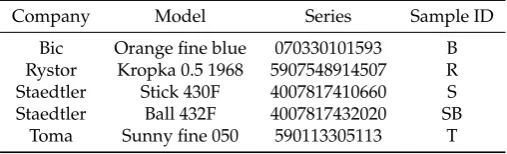
Table 1.List of ballpoint pens used in the experiment.
Company Model Series Sample ID
Bic Orange fine blue 070330101593 B
Rystor Kropka 0.5 1968 5907548914507 R
Staedtler Stick 430F 4007817410660 S
Staedtler Ball 432F 4007817432020 SB
Toma Sunny fine 050 590113305113 T
employed in classification/fitting problems by means of computational intelligence techniques. In 74
a paper by Hoehses et al. [32], the benefit of applying several independent chemometric methods to 75
LIBS data was demonstrated. A consecutive methodology of applying soft independent modelling 76
of class analogy (SIMCA) and partial least-squares discriminant analysis (PLS-DA) enabled the 77
step-wise classification of data and separation of inks that were not identified by principal component 78
analysis (PCA). The SVM yielded a correct classification rate of 87% and cross-validation accuracy 79
amounted to 81%. In the second paper [33], multiple methods such as three comparative functions 80
(linear correlation, overlapping integral, and sum of squared deviations) and two advanced statistical 81
methods (multivariate curve resolution alternating least squares (MCR-ALS) with classification tree and 82
discriminant analysis (DA)) were applied to statistically evaluate LIBS spectra. The newly introduced 83
MCR-ALS/DA methodology showed identification of the paper and printer type with an accuracy of 84
96.3% and 83.3%, respectively. 85
In the present paper, we show that the similar problem can be solved using computational 86
intelligence methods. With our approach much betterDPis achieved and the processing time is greatly 87
reduced. Our results show that the machine learning algorithms can be used to analyze the LIBS 88
spectra. 89
The classification problem discussed in this paper is very difficult due to similarities between 90
LIBS spectra from different paper-ink samples and differences between such spectra from one single 91
class. Additionally, we operate over the long samples with significant noise. To solve this classification 92
problem, we tested many preprocessing ways and computational intelligence methods, however the 93
paper presents only selected and best ones. 94
2. Materials and Methods
95
2.1. Materials 96
Fifty ballpoint pens (10 items of each of 5 models) produced by four different manufacturers from 97
Germany and Poland (more details in Table1) were purchased in Poland. Fifty sheets (10 sheets of 98
each of 5 types) of five Canadian certified reference papers were used (papers denoted A, D, L, N and 99
O from the set “Fillers in paper” supplied by A.S.O. Design Canada). 100
Each particular ink from each of 10 pens of 5 types was deposited (as straight lines) on each of 10 101
sheets of 5 types of papers in the form of straight lines, using standard hand pressure. All 2 500 (50 102
sheets of papers with 50 deposits each) paper-ink samples were placed in plastic bags and stored in 103
darkness at room temperature. 104
In the experiment data for 30 classes (A, A+B, A+R, A+S, A+SB, A+T, D, D+B, . . . , O+SB, O+T) 105
based on the combination of ink, paper and empty papers were recorded. 106
2.2. LIBS 107
The analysis of all paper-ink samples was carried out using a laser induced breakdown 108
spectroscopy system LIBS-6 (Applied Photonics, United Kingdom). It consists of an integrated 109
Q-switched Quantel Ultra Nd-YAG laser (Quantel, France) working at λ = 1 064 nm emitting a 110
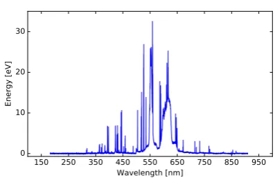
150 250 350 450 550 650 750 850 950 Wavelength [nm]
0 10 20 30
Energy [eV]
×103
Figure 1.Visualization of a signal from the class A.
Czerny-Turner spectrometer (6-channel) with a CCD detector (Avantes, The Netherlands). The system 112
was also equipped with a camera enabled to observe the analyzed object and a movable sample table. 113
The LIBS-6 system was operated by LIBSoft V6.0.1 software (Applied Photonics, United Kingdom). 114
Under normal conditions, because of no moving elements inside, a wavelength calibration of the 115
spectrometer was not required. Every measurments were conducted in air under atmospheric pressure. 116
A Q-switch delay time of 165 µs, the integration delay time of 1.27 µs and integration time of 117
1.2 ms were used. Samples were analysed directly without any special preparation. They were placed 118
at the sample table at the focal point of the focusing lens (at a distance determined by the nozzle about 119
70 mm from the optical head). The diameter of the ablation spot, ranged from 0.6 mm to 1 mm, was 120
dependent on the analysed material. 121
The results of LIBS analysis are an emission spectrum – intensity distribution of the radiation 122
energy (expressed in electron volts) emitted by the analysed object depends on the wavelength 123
measured in nanometres. The emission spectra were collected in the UV-vis range (185 nm to 904 nm, 124
spectral resolution 0.1 nm). 125
In total, 30 classes of experimental data listed above were recorded. For each class 100 LIBS 126
spectra were acquired, resulting in 3 000 samples of the LIBS emission spectrum. A sample spectrum is 127
shown in Figure1. The spectrum of each sample is available on our website [34]. 128
2.3. Data Analysis 129
The analysis of the LIBS spectrum consisted of the following steps: 130
1. Independent preprocessing of LIBS samples. 131
2. Selection of data samples for the cross validation and testing sets. 132
3. Data analysis based on computational intelligence methods. 133
4. Evaluation of the results. 134
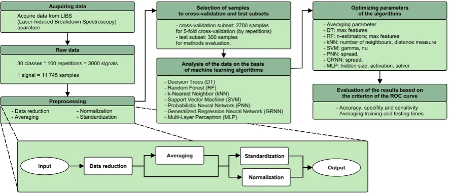
Steps of the experiment are presented in the flowchart in Figure2. 135
2.3.1. Signal preprocessing 136
The initial preprocessing of the raw data was performed to reduce the number of data points 137
corresponding to individual samples of the LIBS spectrum. This preprocessing step was applied 138
because the spectral range of LIBS is very broad (11 746 spectral lines in this case) and from the 139
viewpoint of computational intelligence applied to classification tasks it contains irrelevant information. 140
It can be expected that the reduction of the datasets enhances extraction of characteristic features of the 141
distinctive classes (types of material) [35]. Four preprocessing steps were taken under consideration: 142
• Data reduction by removing the data points from the beginning (first 3 746 data points) and from 143
the end (last 1 000 data points) of the LIBS spectrum, which do not contain relevant information. 144
Figure 2.Flow chart of the experiment.
• Normalization of energy values to the interval[0, 1]. 146
• Standardization of energy values, so the mean value becomes equal to 0 and standard deviation 147
becomes equal to 1. 148
• Application of arithmetic averaging over consecutive numberAP(called averaging parameter) of 149
data points after data reduction and prior to either normalization or standardization. As a result, 150
we reduce the original length of the data vector by a factor ofAP. The tested vales ofAPranged 151
from 5 to 100. 152
Four preprocessing ways based on these steps were constructed and evaluated: data reduction, 153
averaging (applied or not), and either standardization or normalization. These steps are depicted at 154
the bottom of Figure2. 155
Custom software in Python language was developed for data preprocessing tasks. 156
2.3.2. Cross-validation 157
The set of 3 000 LIBS emission spectrum samples was divided into two subsets [36] a training 158
subset containing 90% (2 700) of samples and a test subset containing 10% (300) of samples. Selection 159
of samples for both subsets was performed in a stratified way. The cross-validation subset was used 160
for parameter optimization and then the test subset was used for final evaluation of different types of 161
classifiers with optimized parameters. 162
The 5-fold stratified cross-validation method was applied to build the training and validation 163
data sets. In each of the five analyzed combinations a training set of 72 LIBS spectra from each of 30 164
classes (2 160 in total) and a validation set of 18 LIBS spectra from each of 30 classes (540 in total) were 165
used." 166
Evaluation of the classifiers with optimized parameters was performed separately for each training 167
subset using the test subset. Results of evaluation based on each training subset were obtained by 168
averaging the folds. 169
2.3.3. Computational Intelligence Methods 170
The samples of LIBS spectra, after preprocessing and cross-validation were fed to the classifiers: 171
Generalized Regression Neural Network (GRNN) [37], Probabilistic Neural Network (PNN) [38], 172
Multi-Layer Perceptron (MLP) [39], Support vector machine (SVM) [40], Decision trees (DT) [41], 173
k-nearest neighbour (kNN) classifier [42] and Random forest (RF) [41]. 174
Each method is potentially dependent on a set of parameters that are either quantitative of 175
separately optimized for each machine learning algorithm to receive the lowest number of erroneous 177
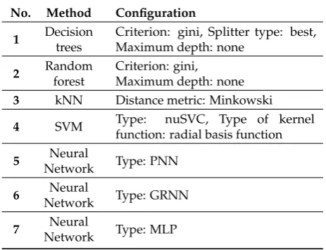
classes. The basic categorical parameters for each method were set to constants listed in Table2. 178
Table 2. Computational intelligence methods and their basic parameters used for LIBS spectra identification.
No. Method Configuration
1 Decision
trees
Criterion: gini, Splitter type: best, Maximum depth: none
2 Random
forest
Criterion: gini, Maximum depth: none
3 kNN Distance metric: Minkowski
4 SVM Type: nuSVC, Type of kernel
function: radial basis function
5 Neural
Network Type: PNN
6 Neural
Network Type: GRNN
7 Neural
Network Type: MLP
Methods based on adaptive neuro-fuzzy inference system (ANFIS) [43] and Gaussian process [44] 179
were also tested, but they are computationally intensive and take long time to receive results even with 180
reduced data set. 181
The custom software developed for this study uses the scikit-learn Python library [45] as a source 182
of implementations of employed computational intelligence algorithms 183
2.3.4. Evaluation criteria 184
Evaluation of classification process was based on methodology described in [46,47]. The 5-fold 185
cross-validation strategy was adopted in our experiment. Five performance parameters namely 186
accuracy (ACC), sensitivity (SEN), specificity (SPE), mean values and Cohen’s kappa (κ) were calculated. 187
The mean values were calculated to estimate the overall performance of the computational intelligence 188
methods used in this study separately for the task of recognition of each of the different classes of LIBS 189
spectra. 190
To test whether there are classes which are classified with higher accuracy, specificity or sensitivity, 191
we calculated for each classSthe number of true positivesTP(S), false positivesFP(S), true negatives 192
TN(S)and false negativesFN(S) separately. Then, the accuracyACC(S), sensitivitySEN(S), and 193
specificitySPE(S)with respect to classSare defined as averages over five folds of cross-validation 194
(K=5 is the number of folds): 195
ACC(S) = 1 K
K
∑
i=1TPi(S) +TNi(S)
TPi(S) +FPi(S) +TNi(S) +FNi(S)
, (1)
SEN(S) = 1 K
K
∑
i=1TPi(S) TPi(S) +FNi(S)
, (2)
SPE(S) = 1 K
K
∑
i=1TNi(S) TNi(S) +FPi(S)
, (3)
whereTPi(S),FPi(S),TNi(S),FNi(S)are, respectively, the number of true positives, false positives, 196
true negatives and false negatives for theith fold of cross-validation with respect to classS,i = 197
150
350
550
750
950
Wavelength [nm]
0
10
20
30
Energy [eV]
×103
(a)Raw data
150
350
550
750
950
Wavelength [nm]
0
10
20
30
Energy [eV]
×103
(b)Reduced data
0
100
200
300
Feature number
0
10
20
30
Energy [eV]
×103
(c)Averaged data (AP=20)
0
100
200
300
Feature number
0.0
0.2
0.4
0.6
Normalized Energy
(d)normalization
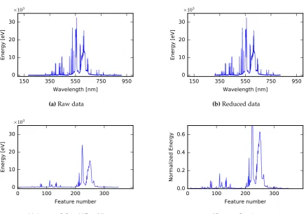
Figure 3.Visualization of data preprocessing for single sample from the class A. Figure (a) depicts an example of a raw spectrogram, (b) shows data after reduction, (c) represents averaged data forAP equal to 20, which is further normalized as shown in (d).
The overall values ofACC,SENandSPEfor the classification system are the arithmetic means of 199
ACC(S),SEN(S)andSPE(S)over all classes. 200
To evaluate the degree of discrimination between two different samples discrimination power 201
coefficient (denotedDP) was proposed [48].DPis the ratio of the number of correctly identified pairs 202
of test samples (identified as from different classes) to the number of all possible pairs of test samples. 203
It can be calculated by the following equation: 204
DP= 2D
T(T−1) =1− 2N
T(T−1), (4)
205
where: 206
• D– the number of differentiated pairs, that is the number of pairs correctly identified as belonging 207
to the same class or correctly identified as belonging to different classes, 208
• N– the number of non-differentiated pairs,N=T(T−1)/2−D, 209
• T– the total number of analysed samples (the total number of possible pairs of samples is equal 210
toT(T−1)/2). 211
3. Results
212
An example of a raw spectrum and the output from successive stages of signal preprocessing 213
(data reduction, averaging, normalization) are shown in Figure3. The averaging stage is optional and 214
The averaging within preprocessing is performed mainly to increase the speed of training and 216
testing, however it can also be described as a feature extraction procedure. Obviously the higherAPis, 217
the faster training and validation are for each of seven tested classification methods. The computation 218
time and classification accuracy were investigated forAPequal to 5, 10, 20, 50, 100, 150, 200 and 219
250. The best trade-off between the number of erroneous classifications and the reduction in the 220
computational time was achieved forAPequal to 20. For this value ofAP, the training computation 221
times were shorter up to 266 times and the testing times were shorter up to 150 times relatively to the 222
processing without averaging (values of speed-up were dependent on the classification method). Thus, 223
forAPequal 20 the number of final spectral lines used decreased from 11 746 to 350. 224
Parameter selection is a key part in reaching the optimal overall performance of a classification 225
system. There are many possible options available, so it is important to analyze the outcomes of 226
experiments for different values of parameters to demonstrate the possibilities of machine learning 227
methods. Particular classification methods depend on the various basic parameters set as listed in 228
Table2and some other parameters that were optimized. Optimization of these parameters was 229
performed in two steps. The first step was to find out the general range of values for each parameter 230
for the fine-tuning procedure. Then the detailed grid search of the selected ranges of parameters was 231
performed. 232
The classification algorithms, the tuning parameters and range of these parameter values are 233
described below. 234
• Decision trees – the number of features to consider when looking for the best split was optimized in 235
two different ranges: from 100 to 7 000 with step equal to 100 when no averaging in preprocessing 236
was done, and from 10 to 350 with step equal to 10 when averaging in preprocessing was 237
performed. 238
• Random forest – two parameters dependent on averaging were optimized during preprocessing. 239
If averaging was not applied, the number of trees in the forest was optimized in range from 10 to 240
200 with step 10 and from 200 to 1 000 with step equal to 50 and the number of features to consider 241
when looking for the best split was optimized in the same range. If averaging was performed, 242
both parameters were optimized in range from 10 to 350 with step 20. 243
• kNN – the number of neighbours was optimized in the range from 1 to 4 and exponent used to 244
calculate the Minkowski distance was optimized from 1 to 10 with step 1. 245
• SVM – the gamma parameter of the RBF kernel function was optimized in range from 0.01 to 1.00 246
with step 0.01 and the nu parameter of the nu-SVC algorithm, related to the error tolerance of the 247
SVM classification, was optimized in range from 0.01 to 1.00 with step 0.01. 248
• PNN – the radius (the spread) of the kernel function of the network (standard deviation for the 249
probability density function of the normal distribution). This parameter was optimized in range 250
from 0.01 to 0.20 with step equal to 0.01 when normalization in preprocessing was used and from 251
0.1 to 1.0 with step 0.1 when standardization was used. 252
• GRNN – the spread parameter with identical meaning and range as in PNN was optimized; 253
• MLP – the number of neurons was optimized in a range from 10 to 200 with step equal to 10. The 254
activation function was selected from ’identity’, ’logistic’, ’tanh’, ’relu’. The solver for weight 255
optimization was chosen from ’lbfgs’ (an optimizer in the family of quasi-Newton methods), ’sgd’ 256
(a stochastic gradient descent) or ’adam’ (a stochastic gradient-based optimizer proposed in [49]). 257
These optimal parameters were selected in a series of experiments to maximize the meanACC,SEN 258
andSPEvalues described in the section2.3.4. 259
The best results of the experiments with different preprocessing methods, machine learning 260
algorithms, based on 5-fold cross-validation (3 000 samples were divided into training set containing 261
2 160 samples, validation set with 540 samples and test sets containing 300) are presented in Table 262
3. The preprocessing involves data reduction, with or without averaging (as in table noted) and 263
standardization. Generally the classification results were worse, when the preprocessing included 264
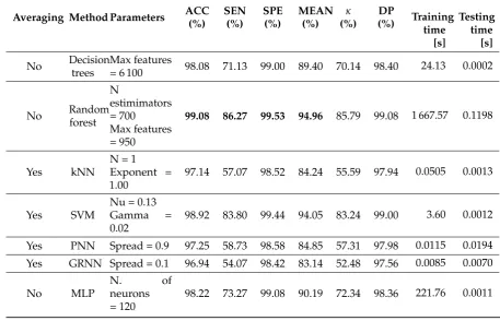
Table 3.Performance results for optimized parameters.
Averaging Method Parameters ACC
(%)
SEN (%)
SPE (%)
MEAN (%)
κ
(%)
DP
(%) Trainingtime
[s]
Testing time
[s]
No Decision trees
Max features
= 6 100 98.08 71.13 99.00 89.40 70.14 98.40 24.13 0.0002
No Random forest
N
estimimators = 700 Max features = 950
99.08 86.27 99.53 94.96 85.79 99.08 1 667.57 0.1198
Yes kNN
N = 1 Exponent = 1.00
97.14 57.07 98.52 84.24 55.59 97.94 0.0505 0.0013
Yes SVM
Nu = 0.13 Gamma = 0.02
98.92 83.80 99.44 94.05 83.24 99.00 3.60 0.0012
Yes PNN Spread = 0.9 97.25 58.73 98.58 84.85 57.31 97.98 0.0115 0.0194 Yes GRNN Spread = 0.1 96.94 54.07 98.42 83.14 52.48 97.56 0.0085 0.0070
No MLP
N. of
neurons = 120
98.22 73.27 99.08 90.19 72.34 98.36 221.76 0.0011
their mean value denotedMEAN),κandDP, and average time of the training for all 5-fold training 266
and testing samples. 267
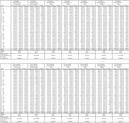
Table4shows the values ofACC(S),SEN(S), andSPE(S)for allSclasses and all classifiers with 268
appropriate preprocessing methods. It can be seen from the table that the most easily distinguishable 269
(highestACC(S),SPE(S)andSEN(S)) samples are in 6 classes: A, A+T, D, N, O and O+T (ACC(S), 270
SPE(S)andSEN(S)reached the value of 100%) using random forest method. Additionally, samples 271
from 2 classes: L and N+T are well recognized by SVM and MLP methods as well. The least 272
distinguishable classes are L+S and O+B with value ofSEN(S) less than 50% by random forest 273
method, howeverSPE(S)value was over 99%. It means that the samples from these classes are often 274
assigned to other classes. 275
The computations were run on a virtual machine with Intel(R) Xeon(R) CPU L5640 @ 2.27 GHz 276
(12 cores without HyperThreading were used) and 20 GB RAM DDR3 1 333 MHz. Independent 277
computations were performed in parallel. The total processing time of each step of computations 278
depends on selected method and its parameters. The training time varied between less than a second 279
for GRNN, PNN and kNN, and almost half an hour for random forest classifiers. The testing time for 280
one sample varied between about 1-2 ms for decision tree and MLP, and more than 0.1 s for random 281
forest, PNN and GRNN classifiers. The time necessary to complete the training was longer but it is 282
less important than the classification speed that is critical at the testing stage. The time required for the 283
identification of a particular sample was less than 1 second (however the exact value depends on the 284
method) and is shown in Table3. 285
4. Discussion
286
The results of experiments confirm that the computational intelligence methods can be used to 287
analyze LIBS data and obtain accurate classification of paper-ink samples (please see Table3). We 288
Table 4.Results of classification per class. Averaging Standardization Decision tree Averaging Standardization Random forest Averaging Standardization kNN Averaging Standardization SVM Averaging Standardization PNN Averaging Standardization GRNN Averaging Standardization MLP Class ACC(%) SPE(%) SEN(%) ACC(%) SPE(%) SEN(%) ACC(%) SPE(%) SEN(%) ACC(%) SPE(%) SEN(%) ACC(%) SPE(%) SEN(%) ACC(%) SPE(%) SEN(%) ACC(%) SPE(%) SEN(%) A 99.33 99.79 86.00 100.00 100.00 100.00 99.80 99.79 100.00 99.87 99.86 100.00 99.20 99.17 100.00 99.67 99.66 100.00 99.60 99.59 100.00 A + B 97.60 98.97 58.00 98.00 99.66 50.00 97.27 98.97 48.00 99.27 99.72 86.00 96.87 99.03 34.00 97.00 99.03 38.00 98.20 99.52 60.00 A + R 97.40 99.10 48.00 98.40 99.93 54.00 97.20 99.79 22.00 99.07 100.00 72.00 97.20 98.62 56.00 96.93 99.24 30.00 98.13 99.31 64.00 A + S 97.20 98.97 46.00 97.80 98.83 68.00 95.73 97.72 38.00 99.07 99.72 80.00 96.07 98.00 40.00 94.33 96.21 40.00 96.60 97.72 64.00 A + SB 95.27 96.62 56.00 95.27 96.21 68.00 94.07 95.59 50.00 97.93 98.48 82.00 94.80 96.90 34.00 94.73 97.03 28.00 96.00 98.07 36.00 A + T 99.33 99.66 90.00 99.87 99.86 100.00 98.93 99.31 88.00 99.20 99.31 96.00 99.00 99.31 90.00 99.00 99.31 90.00 98.73 98.97 92.00 D 99.27 99.38 96.00 99.80 99.79 100.00 99.13 99.24 96.00 99.67 99.66 100.00 98.67 98.83 94.00 99.87 100.00 96.00 99.73 99.86 96.00 D + B 96.20 98.34 34.00 96.60 98.97 28.00 95.07 98.00 10.00 98.20 99.45 62.00 96.13 99.45 0.00 96.20 99.52 0.00 95.53 98.00 24.00 D + R 97.67 98.69 68.00 99.13 99.72 82.00 96.93 98.76 44.00 99.80 99.79 100.00 97.13 99.03 42.00 97.47 98.34 72.00 96.80 97.38 80.00 D + S 96.47 97.79 58.00 98.13 99.03 72.00 94.47 96.48 36.00 99.33 99.93 82.00 95.47 97.79 28.00 94.80 95.79 66.00 95.87 98.76 12.00 D + SB 96.40 98.41 38.00 95.87 97.38 52.00 94.93 97.52 20.00 97.40 98.62 62.00 94.60 96.14 50.00 95.60 98.21 20.00 95.80 98.21 26.00 D + T 98.80 99.24 86.00 99.40 99.38 100.00 98.73 99.31 82.00 99.20 99.24 98.00 98.07 98.69 80.00 99.07 99.38 90.00 99.00 99.10 96.00 L 99.47 99.72 92.00 99.67 99.66 100.00 99.33 99.31 100.00 100.00 100.00 100.00 98.73 98.69 100.00 98.53 98.48 100.00 99.87 99.86 100.00 L + B 96.00 97.72 46.00 97.07 98.34 60.00 95.13 97.72 20.00 98.87 99.52 80.00 95.33 96.34 66.00 95.60 98.41 14.00 97.27 98.41 64.00 L + R 96.73 99.10 28.00 97.20 99.93 18.00 97.53 99.59 38.00 98.80 99.59 76.00 97.13 99.59 26.00 96.87 99.24 28.00 97.07 98.90 44.00 L + S 95.40 97.52 34.00 95.87 97.59 46.00 96.87 98.90 38.00 97.40 99.10 48.00 96.07 98.69 20.00 96.67 98.41 46.00 96.40 98.28 42.00 L + SB 96.13 97.45 58.00 96.73 97.52 74.00 94.67 95.93 58.00 97.53 98.07 82.00 96.47 98.55 36.00 93.80 95.17 54.00 97.67 98.48 74.00 L + T 98.73 99.45 78.00 99.33 99.66 90.00 98.87 99.45 82.00 99.80 99.79 100.00 97.87 98.62 76.00 97.73 99.52 46.00 99.73 99.86 96.00 N 99.27 99.59 90.00 100.00 100.00 100.00 100.00 100.00 100.00 100.00 100.00 100.00 100.00 100.00 100.00 99.67 99.66 100.00 100.00 100.00 100.00 N + B 96.27 98.41 34.00 97.60 99.31 48.00 97.47 99.24 46.00 99.93 100.00 98.00 98.53 99.31 76.00 97.47 99.52 38.00 99.07 99.79 78.00 N + R 96.07 98.34 30.00 97.93 99.45 54.00 96.33 98.00 48.00 97.60 99.31 48.00 96.73 98.41 48.00 95.87 97.93 36.00 97.73 99.03 60.00 N + S 96.20 98.28 36.00 98.60 99.59 70.00 97.00 99.03 38.00 98.47 99.66 64.00 96.80 99.03 32.00 96.73 98.48 46.00 98.20 99.52 60.00 N + SB 94.60 96.41 42.00 95.27 96.34 64.00 96.27 97.31 66.00 97.20 97.52 88.00 96.20 97.66 54.00 95.47 96.90 54.00 96.87 97.59 76.00 N + T 99.13 99.38 92.00 99.67 99.66 100.00 99.47 99.45 100.00 100.00 100.00 100.00 99.07 99.03 100.00 98.53 99.10 82.00 99.73 99.72 100.00 O 99.60 99.93 90.00 100.00 100.00 100.00 99.93 99.93 100.00 100.00 100.00 100.00 100.00 100.00 100.00 99.87 99.86 100.00 100.00 100.00 100.00 O + B 96.93 98.62 48.00 97.93 99.10 64.00 97.13 99.66 24.00 98.67 100.00 60.00 97.47 99.38 42.00 97.20 100.00 16.00 98.53 99.79 62.00 O + R 98.67 99.52 74.00 98.73 99.72 70.00 95.80 97.93 34.00 99.07 99.79 78.00 97.13 98.90 46.00 95.73 98.48 16.00 98.87 99.59 78.00 O + S 96.67 98.34 48.00 98.00 99.66 50.00 95.87 98.14 30.00 98.93 99.38 86.00 96.80 98.34 52.00 96.07 98.34 30.00 98.87 99.38 84.00 O + SB 96.27 97.72 54.00 97.20 97.52 88.00 94.60 95.93 56.00 97.40 97.79 86.00 94.93 96.83 40.00 92.27 93.72 50.00 98.00 98.28 90.00 O + T 99.33 99.38 98.00 99.60 99.59 100.00 99.60 99.59 100.00 99.93 99.93 100.00 99.00 98.97 100.00 99.40 99.52 96.00 100.00 100.00 100.00 Mean 97.41 98.66 61.20 98.16 99.05 72.33 97.14 98.52 57.07 98.92 99.44 83.80 97.25 98.58 58.73 96.94 98.42 54.07 98.13 99.03 71.93
Kappa 59.86 71.38 55.59 83.24 57.31 52.48 70.97
DP 98.13 98.39 97.94 99.00 97.98 97.56 98.53
Training time
(2160 samples) [s] 1.515446 195.209990 0.050514 3.601221 0.011458 0.008476 41.973599 Test time
(1 sample) [s] 0.000120 0.066707 0.001249 0.001212 0.019413 0.007031 0.002214
No averaging Standardization Decision tree No averaging Standardization Random forest No averaging Standardization kNN No averaging Normalization SVM No averaging Normalization PNN No averaging Standardization GRNN No averaging Standardization MLP Class ACC(%) SPE(%) SEN(%) ACC(%) SPE(%) SEN(%) ACC(%) SPE(%) SEN(%) ACC(%) SPE(%) SEN(%) ACC(%) SPE(%) SEN(%) ACC(%) SPE(%) SEN(%) ACC(%) SPE(%) SEN(%) A 99.20 99.45 92.00 100.00 100.00 100.00 100.00 100.00 100.00 100.00 100.00 100.00 99.40 99.38 100.00 99.73 99.72 100.00 99.93 99.93 100.00 A + B 98.60 99.45 74.00 99.33 100.00 80.00 97.53 98.97 56.00 99.27 99.86 82.00 97.40 99.17 46.00 98.53 99.59 68.00 98.60 99.59 70.00 A + R 97.93 99.24 60.00 99.40 99.72 90.00 97.87 99.66 46.00 99.33 100.00 80.00 97.40 99.38 40.00 98.27 99.45 64.00 97.87 98.83 70.00 A + S 96.60 97.93 58.00 99.40 99.72 90.00 96.80 97.86 66.00 99.33 99.72 88.00 96.47 98.69 32.00 97.27 98.07 74.00 96.87 97.86 68.00 A + SB 96.40 97.93 52.00 98.67 98.90 92.00 97.20 98.14 70.00 98.60 98.83 92.00 95.27 95.93 76.00 97.47 98.90 56.00 96.80 98.69 42.00 A + T 98.80 99.72 72.00 100.00 100.00 100.00 99.67 99.72 98.00 99.60 99.59 100.00 98.33 99.31 70.00 99.27 99.38 96.00 99.67 99.72 98.00 D 99.80 99.79 100.00 100.00 100.00 100.00 98.60 98.55 100.00 99.87 99.93 98.00 98.47 98.76 90.00 99.33 99.31 100.00 99.87 99.86 100.00 D + B 98.07 99.03 70.00 99.33 99.72 88.00 95.80 98.48 18.00 98.47 99.59 66.00 95.67 98.28 20.00 96.27 99.31 8.00 95.73 98.28 22.00 D + R 98.40 99.17 76.00 99.93 99.93 100.00 97.80 99.79 40.00 99.73 99.72 100.00 96.67 98.28 50.00 98.20 99.31 66.00 97.93 99.52 52.00 D + S 98.53 99.17 80.00 99.53 100.00 86.00 96.40 97.17 74.00 99.53 99.86 90.00 95.40 97.66 30.00 97.13 97.66 82.00 95.60 97.10 52.00 D + SB 96.67 98.21 52.00 98.80 99.59 76.00 96.07 98.14 36.00 97.73 98.76 68.00 94.60 97.31 16.00 97.40 98.55 64.00 95.73 97.86 34.00 D + T 99.13 99.59 86.00 99.07 99.03 100.00 98.40 99.10 78.00 99.20 99.31 96.00 97.20 98.34 64.00 98.33 98.97 80.00 99.00 99.10 96.00 L 99.40 99.45 98.00 99.53 99.52 100.00 96.27 96.14 100.00 100.00 100.00 100.00 98.80 98.76 100.00 94.67 94.48 100.00 100.00 100.00 100.00 L + B 98.07 99.24 64.00 99.87 99.93 98.00 96.47 99.38 12.00 99.27 99.59 90.00 95.87 97.59 46.00 96.33 99.59 2.00 98.47 99.59 66.00 L + R 97.73 99.45 48.00 98.47 99.93 56.00 96.80 99.45 20.00 98.20 99.24 68.00 96.87 98.90 38.00 96.33 99.59 2.00 97.93 99.72 46.00 L + S 96.00 98.07 36.00 97.20 99.17 40.00 96.00 98.97 10.00 97.47 99.59 36.00 95.80 98.48 18.00 96.47 99.45 10.00 96.73 98.07 58.00 L + SB 95.67 96.55 70.00 96.67 97.10 84.00 91.53 93.45 36.00 97.00 97.52 82.00 94.87 96.34 52.00 91.20 92.97 40.00 97.27 97.66 86.00 L + T 98.07 99.45 58.00 99.20 99.66 86.00 96.00 98.69 18.00 99.53 99.66 96.00 97.93 99.66 48.00 95.27 98.55 0.00 99.60 99.79 94.00 N 99.87 99.93 98.00 100.00 100.00 100.00 99.07 99.03 100.00 100.00 100.00 100.00 100.00 100.00 100.00 98.33 98.28 100.00 100.00 100.00 100.00 N + B 98.33 99.66 60.00 98.73 99.59 74.00 96.93 99.24 30.00 99.67 100.00 90.00 97.47 98.62 64.00 95.67 98.90 2.00 98.80 99.66 74.00 N + R 98.40 99.59 64.00 99.53 100.00 86.00 95.67 98.97 0.00 97.67 99.45 46.00 95.33 97.86 22.00 95.60 98.90 0.00 98.13 99.59 56.00 N + S 97.60 98.55 70.00 99.27 99.93 80.00 97.60 99.52 42.00 98.13 99.45 60.00 95.80 98.34 22.00 96.87 99.72 14.00 98.47 99.17 78.00 N + SB 96.33 97.59 60.00 97.33 98.00 78.00 92.47 93.93 50.00 96.53 96.97 84.00 94.47 96.76 28.00 88.53 90.14 42.00 96.73 97.52 74.00 N + T 99.33 99.45 96.00 99.67 99.66 100.00 99.07 99.38 90.00 100.00 100.00 100.00 99.07 99.17 96.00 96.60 99.38 16.00 100.00 100.00 100.00 O 99.20 99.31 96.00 100.00 100.00 100.00 99.93 99.93 100.00 100.00 100.00 100.00 100.00 100.00 100.00 99.87 99.86 100.00 100.00 100.00 100.00 O + B 96.73 98.90 34.00 97.53 99.93 28.00 96.60 99.93 0.00 98.00 99.86 44.00 97.20 99.38 34.00 96.33 99.66 0.00 97.80 100.00 34.00 O + R 99.47 99.86 88.00 99.67 100.00 90.00 96.60 99.93 0.00 98.93 99.86 72.00 96.53 98.90 28.00 96.27 99.59 0.00 99.00 100.00 70.00 O + S 98.73 99.45 78.00 99.47 99.86 88.00 96.27 99.45 4.00 98.07 99.24 64.00 95.27 98.00 16.00 96.33 99.66 0.00 98.20 98.83 80.00 O + SB 95.87 97.31 54.00 96.93 96.90 98.00 87.93 89.45 44.00 96.00 96.41 84.00 92.87 94.90 34.00 84.67 86.55 30.00 96.13 96.76 78.00 O + T 99.33 99.66 90.00 100.00 100.00 100.00 98.40 98.76 88.00 99.93 99.93 100.00 98.80 98.83 98.00 95.47 98.62 4.00 99.67 99.66 100.00 Mean 98.08 99.00 71.13 99.08 99.53 86.27 96.72 98.31 50.87 98.84 99.40 82.53 96.84 98.37 52.60 96.27 98.07 44.00 98.22 99.08 73.27
Kappa 70.14 85.79 49.17 81.93 50.97 42.07 72.34
DP 98.40 99.08 96.72 98.85 97.80 95.58 98.36
Training time
(2160 samples) [s] 24.133323 1667.572550 3.079269 59.289178 0.102529 0.097161 221.757532 Test time
(1 sample) [s] 0.000187 0.119767 0.023932 0.021494 0.148362 0.142901 0.001074
directly compared with those obtained in [29,30] focusing on the problem of discrimination between 290
two samples which were not assigned to a priori classes. However, the methods used in [29,30] used 291
Plasus SpecLine 2.13 software for the identification of spectral lines and National Institute of Standards 292
and Technology (NIST) spectral database, gave values of theDPin the range from 85% to 92%. The 293
same standard methods with visual spectra was applied to the data collected in our study gaveDP 294
equal to 90.6%. After adopting our algorithms to the problem of discrimination between two different 295
samples, we achieved theDPof 99.0% with SVM and more than 98% with decision trees, random forest, 296
PNN and MLP classifiers. The limitation of applying our solution to the problem of discrimination is 297
that the classes must be predefined. 298
Additionally, application of an automated method based on machine learning greatly reduced the 299
time required for spectrum recognition. The recognition time for a single spectrum was less than 1 300
second. 301
The detailed analysis of the Table3shows that the best method for the class of problems addressed 302
in the present study is the random forest classifier. Parameters for this classifier were optimized using 303
the 5-fold cross-validation using averaged and standardized data. The classifier during test over 304
had no erroneous recognitions in training sets (10 800 cases). This classifier achieved an accuracy of 306
99.08%, sensitivity of 86.27%, specificity of 99.53%, kappa of 85.79% andDPof 99.08% for the test set. 307
Taking into account the number of erroneous classifications under different settings, the worst 308
classifier was GRNN, however it was the fastest classifier during training. 309
Four preprocessing methods were applied on the raw data prior to the classification. Hence, we 310
have shown that the success of classification depends on careful selection of preprocessing procedures. 311
However, although in most cases the actual selection of the pair preprocessing-classifier determines 312
the overall performance of the classification method, for some specific selections of classifier the final 313
classification performance depends only marginally on the preprocessing. For this reason, it is not 314
possible to select a single best preprocessing method. 315
The estimation of an optimalAPfor decision trees,kNN, SVM and GRNN methods will be the 316
subject of the future research. It should be pointed out that the problem of optimal data reduction is 317
important. The length of data series influences the time needed to train the classifiers although it has 318
only marginal effect on the time needed for classification of a test sample. 319
Looking at the spectral data processed in the experiment, the averaging does not seem to be an 320
appropriate preprocessing method for data reduction because the differences between different kinds 321
of samples are inconspicuous. Authors took two other methods into consideration: resampling and 322
wavelet decomposition. The first method resamples the input data at given wavelengths of the original 323
sequence. To obtain 350 samples, resampling withAP= 20 was performed. This method, yielded 324
worse results during identification when averaging step was replaced. The second method performs 325
one dimensional Haar wavelet decomposition [50]. The initial results are promising, however this 326
method requires more detailed investigation in the future. This technique needs further research to 327
determine the type of wavelet decomposition structure and its parameters which will lead to the best 328
results. 329
The results of the present study show that modern computational intelligence methods can 330
be used for the classification of LIBS spectra into predefined classes, which solves a broad class of 331
problems related to LIBS applications. The main limitation of this study is that with the chosen settings 332
another broad class of LIBS applications, that is analysis of elemental composition, cannot be solved. 333
The problem of classification addressed in the present study is certainly simpler than the problem 334
of detailed analysis of the composition of materials. However, successful solution of this problem 335
encourages further research in this area. We suppose, because the problem of analysis of composition 336
of materials based on a LIBS spectrum may occur to be equivalent to the recognition of the presence of 337
specific spectral lines, this problem can be brought to a series of classification subproblems. 338
5. Conclusions
339
The aim of this study is to solve the difficult problem of distinguishing paper-ink samples. Hence, 340
we have designed a computational intelligence system to solve this problem using LIBS spectra. 341
Difficulty of this problem is caused by the high variability of spectra within a single class of paper-ink 342
samples and strong similarity of samples from different classes. 343
A machine learning system is developed and based on results presented in Table3and Table4, 344
we can conclude that the system performed its task for majority of LIBS spectra in a short time. The 345
described method has sensitivity of 86% and it needs to be improved further. The main limitation of 346
this method is that we do not list particular elements of the tested material, however it also should be 347
taken under consideration in future work. Additional feature extraction and classification methods 348
can be applied in the future. 349
Author Contributions:The work presented in this paper was a collaboration of all authors. The manuscript was
350
revised by all authors. Conceptualization, M.K., K.Rz., T.S., and P.P.; Methodology, K.Rz., M.K., and P.P.; Software,
351
T.S.; Validation, K.Rz., and P.P.; Investigation, M.K., K.Rz., T.S., and P.P.; Resources, M.K., M.N., and T.Ł.; Data
352
Curation, M.K., T.S., and P.P.; Writing – Original Draft Preparation, M.K., K.Rz., and P.P.; Writing – Review &
353
Editing, M.B., K.Rz., O.Y., P.P., and R.A.; Visualization, T.S., and P.P.; Supervision, K.Rz., P.P., and R.A.;
Funding:This research received no external funding.
355
Conflicts of Interest:The authors declare no conflict of interest. The founding sponsors had no role in the design
356
of the study; in the collection, analyses, or interpretation of data; in the writing of the manuscript, and in the
357
decision to publish the results.
358
359
1. Singh, J.; Thakur, S.Laser-Induced Breakdown Spectroscopy, 1st ed.; Elsevier The Netherlands: UK, 2007.
360
2. Anabitarte, F.; Cobo, A.; Lopez-Higuera, J.M. Laser-Induced Breakdown Spectroscopy: Fundamentals,
361
Applications, and Challenges. International Scholarly Research Notices Spectroscopy 2012, 2012.
362
doi:10.5402/2012/285240.
363
3. Galbács, G. A critical review of recent progress in analytical laser-induced breakdown spectroscopy.
364
Analytical and Bioanalytical Chemistry2015,407, 7537–7562. doi:10.1007/s00216-015-8855-3.
365
4. Stelmaszczyk, K.; Rohwetter, P.; Méjean, G.; Yu, J.; Salmon, E.; Kasparian, J.; Ackermann, R.; Wolf, J.P.;
366
Wöste, L. Long-distance remote laser-induced breakdown spectroscopy using filamentation in air. Applied
367
Physics Letters2004,85, 3977–3979. doi:http://dx.doi.org/10.1063/1.1812843.
368
5. Wiens, R.; Maurice, S. The ChemCam investigation: compositions at the curiosity rover landing site.
369
Geological Society of America Abstracts with Programs, 2012, Vol. 44, p. 190.
370
6. Ramirez-Cedeno, M.; Ortiz-Rivera, W.; Pacheco-Londono, L.; Hernandez-Rivera, S. Remote Detection of
371
Hazardous Liquids Concealed in Glass and Plastic Containers. Sensors Journal, IEEE2010,10, 693–698.
372
doi:10.1109/JSEN.2009.2036373.
373
7. Noyel, M.; Thomas, P.; Charpentier, P.; Thomas, A.; Brault, T. Implantation of an on-line quality process
374
monitoring. Industrial Engineering and Systems Management (IESM), Proceedings of 2013 International
375
Conference on, 2013, pp. 1–6.
376
8. Ortiz, R.; Ortiz, P.; Colao, F.; Fantoni, R.; Gómez-Morón, M.; Vázquez, M. Laser spectroscopy and imaging
377
applications for the study of cultural heritage murals. Construction and Building Materials2015,98, 35 – 43.
378
doi:10.1016/j.conbuildmat.2015.08.067.
379
9. Rinke-Kneapler, C.; Sigman, M. 15 - Applications of laser spectroscopy in forensic science. In
380
Laser Spectroscopy for Sensing; Baudelet, M., Ed.; Woodhead Publishing, 2014; pp. 461 – 495.
381
doi:10.1533/9780857098733.3.461.
382
10. Król, M.; Kowalska, D.; Ko´scielniak, P. Examination of Polish Identity Documents
383
by Laser-Induced Breakdown Spectroscopy. Analytical Letters 2018, 51, 1592–1604,
384
[https://doi.org/10.1080/00032719.2017.1384833]. doi:10.1080/00032719.2017.1384833.
385
11. Gaft, M.; Sapir-Sofer, I.; Modiano, H.; Stana, R. Laser induced breakdown spectroscopy for bulk minerals
386
online analyses. Spectrochimica Acta Part B: Atomic Spectroscopy2007,62, 1496 – 1503. A Collection of Papers
387
Presented at the 4th International Conference on Laser Induced Plasma Spectroscopy and Applications
388
(LIBS 2006), doi:10.1016/j.sab.2007.10.041.
389
12. Anabitarte, F.; Mirapeix, J.; Portilla, O.M.C.; Lopez-Higuera, J.M.; Cobo, A. Sensor for the Detection of
390
Protective Coating Traces on Boron Steel With Aluminium–Silicon Covering by Means of Laser-Induced
391
Breakdown Spectroscopy and Support Vector Machines. IEEE Sensors Journal 2012, 12, 64–70.
392
doi:10.1109/JSEN.2011.2121902.
393
13. Bukin, O.; Proschenko, D.; Chekhlenok, A.; Golik, S.; Bukin, I.; Mayor, A.; Yurchik, V. Laser
394
Spectroscopic Sensors for the Development of Anthropomorphic Robot Sensitivity. Sensors2018,18.
395
doi:10.3390/s18061680.
396
14. Moncayo, S.; Manzoor, S.; Navarro-Villoslada, F.; Caceres, J.O. Evaluation of supervised chemometric
397
methods for sample classification by Laser Induced Breakdown Spectroscopy.Chemometrics and Intelligent
398
Laboratory Systems2015,146, 354–364. doi:10.1016/j.chemolab.2015.06.004.
399
15. Zhang, T.; Xia, D.; Tang, H.; Yang, X.; Li, H. Classification of steel samples by laser-induced breakdown
400
spectroscopy and random forest. Chemometrics and Intelligent Laboratory Systems2016, 157, 196–201.
401
doi:10.1016/j.chemolab.2016.07.001.
402
16. Wang, N.; Wang, X.; Chen, P.; Jia, Z.; Wang, L.; Huang, R.; Lv, Q. Metal Contamination Distribution
403
Detection in High-Voltage Transmission Line Insulators by Laser-induced Breakdown Spectroscopy (LIBS).
404
Sensors2018,18. doi:10.3390/s18082623.
17. Zhang, C.; Shen, T.; Liu, F.; He, Y. Identification of Coffee Varieties Using Laser-Induced Breakdown
406
Spectroscopy and Chemometrics. Sensors2018,18. doi:10.3390/s18010095.
407
18. Tognoni, E.; Palleschi, V.; Corsi, M.; Cristoforetti, G.; Omenetto, N.; et al., I.G., Laser-induced breakdown
408
spectroscopy (LIBS) fundamentals and applications; New York, USA: Cambridge University Press, 2006;
409
chapter From sample to signal in laser-induced breakdown spectroscopy: a complex route to quantitative
410
analysis, p. 122.
411
19. Tadeusiewicz, R. Place and Role of Intelligent Systems in Computer Science.Computer Methods in Materials
412
Science2010,10, 193–206.
413
20. Pławiak, P.; So´snicki, T.; Nied´zwiecki, M.; Tabor, Z.; Rzecki, K. Hand Body Language Gesture Recognition
414
Based on Signals From Specialized Glove and Machine Learning Algorithms.IEEE Transactions on Industrial
415
Informatics2016,12, 1104–1113. doi:10.1109/TII.2016.2550528.
416
21. Pławiak, P. An estimation of the state of consumption of a positive displacement pump based
417
on dynamic pressure or vibrations using neural networks. Neurocomputing 2014, 144, 471 – 483.
418
doi:https://doi.org/10.1016/j.neucom.2014.04.026.
419
22. Pławiak, P.; Maziarz, W. Classification of tea specimens using novel hybrid artificial intelligence methods.
420
Sensors and Actuators B: Chemical2014,192, 117 – 125. doi:10.1016/j.snb.2013.10.065.
421
23. Rzecki, K.; Pławiak, P.; Nied´zwiecki, M.; So´snicki, T.; Le´skow, J.; Ciesielski, M. Person recognition based
422
on touch screen gestures using computational intelligence methods.Information Sciences2017,415–416, 70 –
423
84. doi:10.1016/j.ins.2017.05.041.
424
24. Pławiak, P.; Rzecki, K. Approximation of Phenol Concentration Using Computational Intelligence
425
Methods Based on Signals From the Metal-Oxide Sensor Array. Sensors Journal, IEEE2015,15, 1770–1783.
426
doi:10.1109/JSEN.2014.2366432.
427
25. Pławiak, P. Novel methodology of cardiac health recognition based on ECG signals
428
and evolutionary-neural system. Expert Systems with Applications 2018, 92, 334 – 349.
429
doi:https://doi.org/10.1016/j.eswa.2017.09.022.
430
26. Pławiak, P. Novel genetic ensembles of classifiers applied to myocardium dysfunction
431
recognition based on ECG signals. Swarm and Evolutionary Computation 2018, 39, 192 – 208.
432
doi:https://doi.org/10.1016/j.swevo.2017.10.002.
433
27. Abdar, M.; Zomorodi-Moghadam, M.; Das, R.; Ting, I.H. Performance analysis of classification
434
algorithms on early detection of liver disease. Expert Systems with Applications2017, 67, 239 – 251.
435
doi:https://doi.org/10.1016/j.eswa.2016.08.065.
436
28. Trejos, T.; Flores, A.; Almirall, J.R. Micro-spectrochemical analysis of document paper and gel inks by
437
laser ablation inductively coupled plasma mass spectrometry and laser induced breakdown spectroscopy.
438
Spectrochimica Acta Part B: Atomic Spectroscopy2010,65, 884 – 895. doi:10.1016/j.sab.2010.08.004.
439
29. Kula, A.; Wietecha-Posłuszny, R.; Pasionek, K.; Król, M.; Wo´zniakiewicz, M.; Ko´scielniak, P. Application of
440
laser induced breakdown spectroscopy to examination of writing inks for forensic purposes. Science &
441
Justice2014,54, 118 – 125. doi:10.1016/j.scijus.2013.09.008.
442
30. Elsherbiny, N.; Nassef, O.A. Wavelength dependence of laser induced breakdown spectroscopy (LIBS) on
443
questioned document investigation.Science & Justice2015,55, 254 – 263. doi:10.1016/j.scijus.2015.02.002.
444
31. Lennard, C.; El-Deftar, M.M.; Robertson, J. Forensic application of laser-induced breakdown spectroscopy
445
for the discrimination of questioned documents. Forensic Science International 2015, 254, 68 – 79.
446
doi:10.1016/j.forsciint.2015.07.003.
447
32. Hoehse, M.; Paul, A.; Gornushkin, I.; Panne, U. Multivariate classification of pigments and inks using
448
combined Raman spectroscopy and LIBS. Analytical and Bioanalytical Chemistry2011, 402, 1443–1450.
449
doi:10.1007/s00216-011-5287-6.
450
33. Metzinger, A.; Rajkó, R.; Galbács, G. Discrimination of paper and print types based on their laser
451
induced breakdown spectra. Spectrochimica Acta Part B: Atomic Spectroscopy 2014, 94–95, 48 – 57.
452
doi:http://dx.doi.org/10.1016/j.sab.2014.03.006.
453
34. Team of Science and Industrial Intelligent Applications; subsection “Research” in:.
454
35. Zieli ´nski, T.P.Digital signal processing: from theory to applications; WK Ł, 2005.
455
36. Murphy, K.P.Machine learning: a probabilistic perspective, 1st ed.; The MIT Press: Cambridge, MA, 2012.
456
37. Specht, D.F. A general regression neural network.IEEE Transactions on Neural Networks1991,2, 568–576.
457
doi:10.1109/72.97934.
38. Specht, D.F. Probabilistic neural networks. Neural Networks 1990, 3, 109–118.
459
doi:doi.org/10.1016/0893-6080(90)90049-Q.
460
39. Hinton, G.E. Connectionist Learning Procedures. Artif. Intell. 1989, 40, 185–234.
461
doi:10.1016/0004-3702(89)90049-0.
462
40. Cortes, C.; Vapnik, V. Support-vector networks. Machine Learning 1995, 20, 273–297.
463
doi:10.1007/BF00994018.
464
41. James, G.; Witten, D.; Hastie, T.; Tibshirani, R.An Introduction to Statistical Learning: With Applications in R;
465
Springer Publishing Company, Incorporated, 2014.
466
42. Altman, N.S. An introduction to kernel and nearest-neighbor nonparametric regression. The American
467
Statistician1992,46, 175–185. doi:10.1080/00031305.1992.10475879.
468
43. Sugeno, M.Industrial applications of fuzzy control; Elsevier Science Pub. Co., 1985.
469
44. Rasmussen, C.E.; Williams, C.K.I.Gaussian Processes for Machine Learning (Adaptive Computation and Machine
470
Learning); The MIT Press, 2005.
471
45. Pedregosa, F.; Varoquaux, G.; Gramfort, A.; Michel, V.; Thirion, B.; Grisel, O.; Blondel, M.; Prettenhofer, P.;
472
Weiss, R.; Dubourg, V.; Vanderplas, J.; Passos, A.; Cournapeau, D.; Brucher, M.; Perrot, M.; Duchesnay, E.
473
Scikit-learn: Machine Learning in Python. Journal of Machine Learning Research2011,12, 2825–2830.
474
46. Fawcett, T. An Introduction to ROC Analysis. Pattern Recognition Letters 2006, 27, 861––874.
475
doi:doi.org/10.1016/j.patrec.2005.10.010.
476
47. Sokolova, M.; Lapalme, G. A systematic analysis of performance measures for classification tasks.
477
Information Processing & Management2009,45, 427 – 437. doi:10.1016/j.ipm.2009.03.002.
478
48. Trejos, T.; Corzo, R.; Subedi, K.; Almirall, J. Characterization of toners and inkjets by
479
laser ablation spectrochemical methods and Scanning Electron Microscopy-Energy Dispersive
480
X-ray Spectroscopy. Spectrochimica Acta Part B: Atomic Spectroscopy 2014, 92, 9 – 22.
481
doi:https://doi.org/10.1016/j.sab.2013.11.004.
482
49. Kingma, D.P.; Ba, J. Adam: A Method for Stochastic Optimization. CoRR2014,abs/1412.6980,[1412.6980].
483
50. Chui, C.K.An Introduction to Wavelets; Academic Press Professional, Inc.: San Diego, CA, USA, 1992.
484
Sample Availability:LIBS spectra used in this study are available on the webpage:http://libs.iti.pk.edu.pl/.