R E S E A R C H
Open Access
Some fast projection methods based on
Chan-Vese model for image segmentation
Jinming Duan
*, Zhenkuan Pan, Xiangfeng Yin, Weibo Wei and Guodong Wang
Abstract
The Chan-Vese model is very popular for image segmentation. Technically, it combines the reduced Mumford-Shah model and level set method (LSM). This segmentation problem is solved interchangeably by computing a gradient descent flow and expensively and tediously re-initializing a level set function (LSF). Though many approaches have been proposed to overcome the re-initialization problem, the low efficiency for this segmentation problem is still not solved effectively. In this paper, we first investigate the relationship between theL1-based total variation (TV) regularizer term of Chan-Vese model and the constraint on LSF and then propose a new technique to solve the re-initialization problem. In detail, four fast projection methods are proposed, i.e., split Bregman projection method (SBPM), augmented Lagrangian projection method (ALPM), dual split Bregman projection method (DSBPM), and dual augmented Lagrangian projection method (DALPM). These four methods without re-initialization are faster than the existing approaches. Finally, extensive numerical experiments on synthetic and real images are presented to validate the effectiveness and efficiency of these four proposed methods.
Keywords:Variational level set method; Chan-Vese model; Re-initialization; Projection method
1. Introduction
Image segmentation is a popular research topic in image processing, as it has a number of significant applications in object detection and moving object tracking, re-sources classification in SAR images, organs segmenta-tion and 3D reconstrucsegmenta-tion in medical images, etc. Among the segmentation approaches, the variational models [1-4] are one of the influential and effective methods. In detail, the Snake model [5] and Mumford-Shah model [6] are two fundamental models for image segmentation using variational method. The first one is a typical parametric active contour model based on image edges and fast for segmentation. However, this parametric model is not very effective for images with weak edge and meanwhile fails to deal with adaptive top-ologies. The second one is a typical region-based model, which aims to replace the original image with a piece-wise smooth image and a minimum contour for image segmentation by minimizing an energy functional. The-oretically, it is very difficult to optimize this Mumford-Shah functional as it includes two energy terms defined
in two-dimensional image space and one-dimensional contour space respectively. In order to implement this model numerically, Aubert et al. [7-9] introduced the concept of shape derivative and transformed the two-dimensional energy term into one-two-dimensional one. Consequently, the original model becomes a parametric active contour model. Different from [5], authors in [7-9] developed a level set scheme [10] to achieve curve evolution for adaptive topologies. Another routine to optimize the Mumford-Shah model is to transform the term in contour space into the one in image space, which can be achieved via introducing a proper charac-teristic function for each different phase that represents different feature in an image. An equivalent energy func-tional of the original Mumford-Shah model was pro-posed in [11] via elliptic function approximation based on convergence theory. Then, this new Gamma-convergence approximated Mumford-Shah model was ex-tended to segment multiphase images [12-14], which forms the first Gamma-convergence family for variational image segmentation. The second family is variational level set method (VLSM) [15] that combines classical LSM and variational method. The most famous model of this family is Chan-Vese model [16], the first one making use of
* Correspondence:[email protected]
College of Information Engineering, Qingdao University, Qingdao 266071, China
Heaviside function of LSF to design characteristic function and then realize two-phase piecewise constant image seg-mentation. Also, this model has been successfully extended for a great number of multiphase image segmentation [17-19]. The third family is variational label function method (VLFM) sometimes also called piecewise constant level set method [20-22] or fuzzy membership function method [23]. However, if the Heaviside function of LSF is considered as a label function, the third family is actually an extended version of the second one.
Technically, the energy functional minimization for image segmentation results in a set of partial differential equations (PDEs), which must be solved numerically. Compared with other traditional methods, the computa-tional efficiency of variacomputa-tional image segmentation model is much slower, so developing its fast numerical algorithms is always a challenging task in this area. Traditionally, the models in the first two families are usually solved by gradient descent flow. Therefore, the resulting Euler equations always include complicated curvature term, which usually leads to slow computa-tional efficiency. Previously, some fast algorithms for op-timizingL1-based total variation (TV) term have already been efficiently applied to the models of third family (VLFM). For example, novel split Bregman algorithm [24,25], dual method [26,27], and augmented Lagrangian method [21,22,28], and these fast algorithms all avoid computing complex curvature associated with TV regu-larizer term. Therefore, these proposed algorithms can improve the convergent rate to a great extent.
For the second family, the VLSM for image segmenta-tion usually uses zero level set of a continuous sign dis-tance function (SDF) to represent a contour and the geometric features (i.e., normal and curvature) can be cal-culated naturally via SDF. Along this way, the post-processing of curves and surfaces will be very convenient. However, the LSF is not preserved as a SDF anymore in the contour evolution and thus the geometric virtue on zero level set will be lost. There are two methods [29,30] to overcome this problem: the traditional one is periodic-ally re-initializing the LSF as a SDF by solving a static eikonal equation or a dynamical Hamilton-Jacobi equation using upwind scheme [29,31-33]. However, this is very expensive and tedious and may make the zero level set moving to undesired positions. The novel one is by con-straining LSF to remain a SDF during the contour evolu-tion through adding penalty terms into the original energy functional [30,34]. However, the penalty parameter limits the time step for the LSF evolution due to Courant-Friedrichs-Lewy (CFL) condition [35] and thus the SDF cannot be preserved unless penalty parameter is very large, which cannot guarantee the stability of numerical computation. In order to avoid CFL condition, researchers in [36] proposed completely augmented Lagrangian method
by introducing eight auxiliary variables and four penalty parameters, leading to numerous sub-minimization and sub-maximization problems for every introduced variable. Therefore, the resulting models are very complicated.
In this paper, we investigate the relationship between the TV regularizer term of Chan-Vese model and the constraint of LSF as a SDF and then propose a new model with fewer auxiliary variables in comparison with [36]. In this case, we can transform the constraint into a very simple algebra equation that can be explicitly im-plemented via direct projection approach without re-initialization. Based on this explicit model and novel technique, three algorithms in the third family (i.e., split Bregman algorithm, dual method, and augmented Lagrangian method) for optimizing the variational models can be conveniently extended to Chan-Vese model in second family, and thus four fast algorithms are devel-oped (i.e., split Bregman projection method, augmented Lagrangian projection method, dual split Bregman projec-tion method, and dual augmented Lagrangian projecprojec-tion method). Technically, the resulting equations in the pro-posed four algorithms include four components: (1): a simple Lagrange equation for LSF and this Euler-Lagrange equation can be solved via fast Gauss-Seidel iter-ation, (2): a generalized soft thresholding formula in analytical form, (3): a fast iterative formula for dual vari-able, and (4): a very simple projection formula. These four components can be used elegantly to avoid computing the complex curvature in [16,30,34]. In addition, all the four proposed fast projection methods can preserve full LSF as a SDF precisely without a very large penalty parameter due to the introduced Lagrangian multiplier and Bregman iterative parameter. So a relatively large time step is allowed to be employed to speed up LSF evaluation in comparison with [30,34]. Most importantly, even if the LSF is initialized as a piecewise constant function, it can be corrected automatically due to the iterative projection computation. Therefore, our proposed methods have both higher computational efficiency and better SDF fidelity than those reported in [30,34,36]. What is worth mention-ing here is that our proposed algorithms are quite generic and can be easily extended to all models using VLSM for multiphase image segmentation, motion segmentation, 3D reconstruction etc. For example, the case [37] for multi-phase image segmentation has been investigated by using augmented Lagrangian projection method in our recent work.
method (DALPM) are presented. In Section 4, extensive numerical experiments have been conducted to compare our proposed fast methods with some existing approaches. Finally, concluding remarks and outlooks are given.
2. The Chan-Vese model and its traditional solution scheme
2.1 Mumford-Shah model
We first introduce the Mumford-Shah model that is the basic of this paper, and it can be discussed below. For a scalar image f(x): Ω→R, the Mumford-Shah model can be stated as the following energy functional minimization problem
Min
u;Γ E uð ;ΓÞ¼α Z
Ωðu−fÞ
2
dxþβ
Z
Ω=Γj j∇u
2
dxþγ
Z
Γds
ð1Þ
wherefis the original input image. The objective of this model is to find a piecewise smooth imageuand a mini-mum contour Γ to minimize (1). α, β, and γ are three positive penalty parameters. This problem is hard to solve due to inconsistent dimensionμandΓ. In order to solve Equation1approximately, Chan and Vese [16] first combined the reduced Mumford-Shah model [6] and VLSM [10] and proposed the following Chan-Vese model with an idea of dividing an image into two regions
Min
u;Γ E uð ;ΓÞ ¼α1 Z
Ω1 u1−f
ð Þ2
dxþα2 Z
Ω2 u2−f
ð Þ2
dxþγ
Z
Γds
ð2Þ
where u= (u1, u2) stands for piecewise constant image mean value in regionsΩ1andΩ2, respectively, andΩ=Ω1 ∪Ω2,Ω1∩Ω2=∅.
2.2 Traditional LSM
In order to understand the Chan-Vese model clearly, let us first recall some concepts of traditional LSM. Γ(t) is defined as a closed contour that separates two regions Ω1(t) andΩ2(t), and a Lipschitz continuous LSFϕ(x,t) is
defined as
ϕð Þx;t >0 x∈Ω1ð Þt ϕð Þ ¼x;t 0 x∈Γð Þt
ϕð Þx;t <0 x∈Ω2ð Þt 8
<
: ð3Þ
whereΓ(t) corresponds to zero level set {x:ϕ(x,t) = 0} and its evolution equation can be transformed into zero level set ofϕ(x,t). Then, we differentiateϕ(x,t) = 0 with respect totand obtain the following LSF evolution equation
ϕtþdx
dt⋅∇ϕ¼0 ð4Þ
As the normal on {x:ϕ(x,t) = 0} is N→¼∇ϕ=j∇ϕj, Equation 4 can be rewritten as the following standard level set evolution equation:
ϕtþvNj∇ϕj ¼0 ð5Þ
where normal velocityvNofΓ(t) isdx dt⋅
∇ϕ ∇ϕ
j j.
Usually,ϕ(x,t) is defined as a SDF
ϕð Þ ¼x;t d xð ;Γð Þt Þ x∈Ω1ð Þt ϕð Þ ¼x;t 0 x∈Γð Þt
ϕð Þ ¼x;t −d xð ;ð Þt Þ x∈Ω2ð Þt 8
< :
ð6Þ
Where d(x, Γ(t)) denotes the Euclidean distance from x to Γ(t). An equivalent constraint to Equation 6 is the eikonal equation
∇ϕð Þx;t
j j ¼1 ð7Þ
In order to satisfy Equation 7, an iterative re-initialization scheme [16] is used to solve the steady state of following equation:
ϕtþsignð Þϕ0 ðj∇ϕj−1Þ ¼0 inΩR
ϕðx;0Þ ¼ϕ0 inΩ
ð8Þ
where ϕ0is the function to be reinitialized and sign(ϕ0)
denotes the sign function ofϕ0.
2.3 The Chan-Vese model under VLSM framework and its solution
By using Heaviside function of LSF and its total variation form, Chan and Vese [16] transformed the model (2) into VLSM. In fact, a Heaviside function is defined as
H xð Þ ¼ 10 otherwisex≥0
ð9Þ
Its derivative in the distributional sense is the Dirac function
δð Þ ¼x ∂H x∂ð Þ
x ð10aÞ
According to Equation 9, the characteristic function of Ω1andΩ2can be defined as
χ1ð Þ ¼x Hðϕð Þx Þ ¼ 10 otherwisex∈Ω1
ð10bÞ
χ2ð Þ ¼x 1−Hðϕð Þx Þ ¼
1 x∈Ω2 0 otherwise
ð10cÞ
γ Z
Γds¼γ Z
Ωj∇Hð Þϕ jdx¼γ Z
Ωj∇ϕjδ ϕð Þdx ð11Þ
Therefore, Equation 2 can be rewritten as the follow-ing VLSM:
Min ϕ;u
Eðϕ;u1;u2Þ ¼α1 Z
Ωðu1−fÞ 2
Hð Þϕ dx
þα2 Z
Ωðu2−fÞ 2
1−Hð Þϕ
ð Þdx
þγ Z
Ωj∇ϕjδ ϕð Þdx
ð12Þ
Equation 12 is a multivariate minimization problem and usually solved via alternative optimization proced-ure. First fixϕto optimizeuand then fixufor optimiz-ingϕ. In detail, whenϕis fixed, we obtain
u1¼ Z
ΩfHð Þϕ dx Z
ΩHð Þϕ dx
; u2¼ Z
Ωfð1−Hð Þϕ Þdx Z
Ωð1−Hð Þϕ Þdx
ð13Þ
On the other hand, when u is fixed, the sub-problem of optimization with respect toϕis as follows:
Min
ϕ Eð Þ ¼ϕ
Z
ΩQ12ðu1;u2ÞHð Þϕ dxþγ Z
Ωj∇Hð Þϕ jdx
ð14Þ
where Q12(u1,u2) =α1(u1−f)2−α2(u2−f)2. In order to
solve Equation 14, we need to compute the evolution equation ofϕvia gradient descent flow as
∂ϕ
∂t ¼ γ∇⋅ ∇ϕ
∇ϕ j j
−Q12ðu1;u2Þ
δ ϕð Þ inΩ
∂ϕ
∂n→¼0 on∂Ω
8 > > < > > :
ð15Þ
In order to avoid singularity in numerical implementa-tion for Equaimplementa-tion 15, the Heaviside funcimplementa-tion and Dirac function are usually approximated by their regularized version with a small positive regularized parameterεas
Hεð Þ ¼ϕ 1
2þ 1 πarctan
ϕ
ε ð16aÞ
δεð Þ ¼ϕ π1ϕ2þε ε2 ð16bÞ
As both the energy functional (12) and the evolution Equation 15 do not include any exact definition of LSF ϕas a SDF, theϕ will not be preserved as a SDF during the contour evolution, which leads to accuracy loss in curve or surface expression.
The first correction approach to preserve the LSF as a SDF is solving Equation 8 using upwind scheme after
some iterations of ϕ using Equation 15. However, this method is expensive and may cause the interface to shrink and move to undesirable positions. In order to make comparisons with other methods, we name this re-initialization approach as gradient descent equation with re-initialization method (GDEWRM).
The second correction approach, which was proposed by [30] as following, is to add the constraint Equation 7 as a penalty term into Equation 14 in order to avoid the tedious re-initialization process
Min
ϕ
Eð Þ ¼ϕ
Z
ΩQ12Hεð Þϕ dxþγ Z
Ωj∇Hεð Þϕ jdx þμ
2 Z
Ωðj∇ϕj−1Þ
2
dx
ð17Þ
Theoretically,μshould be a large penalty parameter in order to sufficiently penalize the constraint |∇ϕ| = 1 as a SDF. However, under such circumstance, we cannot choose a relatively large time step to improve the com-putational efficiency due to the CFL stability condition [35]. Here, we name this method as gradient descent equation without re-initialization method (GDEWORM).
As an extension of (17), an augmented Lagrangian method (ALM) and a projection Lagrangian method (PLM) are proposed by [34] to remain the LSF as a SDF during the LSF evolution. These two extensions can be expressed as follows, respectively:
Min
ϕ
Eðϕ;λÞ ¼ Z
ΩQ12Hεð Þϕ dxþγ Z
Ωj∇Hεð Þϕ jdx þ
Z
Ωλðj∇ϕj−1Þdxþ μ 2
Z
Ωðj∇ϕj−1Þ 2
dx
ð18Þ
Min ϕ;w→
E ϕ;w→
¼ Z
ΩQ12Hεð Þϕ dxþγ Z
Ωj∇Hεð Þϕ jdx þ
Z
Ωλ w → −1
dxþμ 2 Z Ω w → −∇ϕ 2 dx
ð19Þ
Different from GDEWORM, ALM (18) enforces the constraint |∇ϕ| = 1 via Lagrangian parameter λ. There-fore, a relatively small penalty parameter μ can be chosen to improve the stability of numerical calculation of Equation 18. The PLM (19) is actually proposed by combining variable splitting and penalty approach, so it is more efficient than GDEWORM due to the split tech-nique. However, one drawback still exists: asμ becomes very large, the intermediate minimization process of PLM becomes increasingly ill-conditioned as happened for GDEWORM.
Using the similar idea, [36] introduced four auxiliary variables and four Lagrangian multipliers to deal with the same constrained optimization problem. The minimization problem is reformulated as following, and here, we name it as completely augmented Lagrangian method (CALM).
E ϕ;φ;s;→v;w→
¼ Z
ΩQ12sdxþγ Z Ω v → dx þZ
Ωλ2ðs−Hεð ÞφÞdxþ μ2
2 Z
Ωðs−Hεð Þφ Þ 2 dx þ Z Ωλ →
3⋅ v →−∇
s
dxþμ3 2 Z Ω v →−∇ s 2 dx þZ
Ωλ1ðφ−ϕÞdxþ μ1 2 Z Ωðφ−ϕÞ 2 dx þZ Ωλ →
4⋅ w →−∇ϕ
dxþμ4 2 Z Ω w →−∇ϕ 2 dx
ð20Þ
s:t w→¼1: ð21Þ
Note that all of the above methods, GDEWRM (8, 14), GDEWORM (17), ALM (18), and PLM (19), only take efforts in how to add the constraint |∇ϕ| = 1 into the original functional and ignore the TV regularizer term∫Ω| ∇H(ϕ)|dx. Therefore, their resulting evolution equations bring about complex curvature terms, and the com-putational efficiency will be very slow due to such compli-cated finite difference scheme for the curvature. Through introducing eight variables in CALM (20), each sub-minimization or sub-maximization problem of this model becomes very simple because there is no curvature term in these sub-problems. However, as we know, every vari-able including Lagrangian multiplier is defined in the do-main of image space, which implies the more variables the model has, the less efficient it will become. Moreover, there are five penalty parameters setting up in the CALM, so the choices of these parameters are more difficult. In order to avoid computing curvature and meanwhile de-crease the number of the introduced variables and param-eters, we will design fast algorithms in the next section, by taking into full consideration the relationship between regularization term ∫ Ω|∇H(ϕ)|dx and constraint term |∇ϕ| = 1.
3. Four fast projection methods
The fast split Bregman method [24,25], dual method [26], and augmented Lagrangian method [28] proposed for TV model for image restoration have been success-fully extended to the Chan-Vese model under VLFM framework [20,38], but they cannot be directly applied to Chan-Vese model under VLSM framework due to the complex constraint |∇ϕ| = 1. In this section, inspired by these fast algorithms, we aim to design some new fast algorithms for Chan-Vese model [16] without re-initialization under VLSM framework. Through
introducing two or three auxiliary variables, the con-straint is transformed into a very simple projection for-mula so that our proposed fast methods are able to avoid both expensive re-initialization process and com-plex curvature appearance in the evolution equations. Therefore, the proposed methods are faster than their counterparts with higher performance.
In order to state the problem clearly, we rewrite the traditional Chan-Vese model (14) and the constraint (7) as the following:
Min
ϕ Eð Þ ¼ϕ Z
ΩQ12ðu1;u2ÞHεð Þϕ dxþγ Z
Ωj∇ϕjδεð Þϕ dx
ð22aÞ
s:t:j∇ϕj ¼1: ð22bÞ
Next, we will introduce each fast algorithm separately.
3.1 Split Bregman projection method
Unlike Equations 18 and 19, we do not put the constraint Equation 22b directly into functional Equation 22a. In-stead, we introduce an auxiliary splitting variablew→ to re-place the ∇ϕin the TV regularizer term∫Ω|∇ϕ|δε(ϕ)dx. Therefore, the constraint Equation 22b becomes
con-straint w→¼1 and another constraint w→¼∇ϕ is
pro-duced. Then, we use the Bregman distance technique [25]
by introducing Bregman iterative parameter →b to satisfy the constraintw→¼∇ϕ, so we can transform Equation 22a, b into the following optimization problem:
Min ϕ;w→
E ϕ;w→
¼ Z
ΩQ12ðu1;u2ÞHεð Þϕ dxþγ Z
Ωw →
δεð Þϕ dx
þθ 2 Z
Ω w−∇ϕ−b →
dx
;
s:t:w→¼1;
In order optimize the above problem, we use the itera-tive technique as
ϕkþ1;
w→kþ1
¼ arg min
ϕ;w→
E ϕ;w→
¼ Z
ΩQ12ðu1;u2ÞHεð Þϕ dx þγZ
Ω w
→
δεð Þϕ dxþθ
2 Z
Ω
w−∇ϕ−→bkþ1
dx
;
ð23aÞ
whereθ> 0 is a penalty parameter, w→ and →b are vectors,
b →kþ1
¼→bkþ∇ϕk−w→k; →b0¼w→0¼→0: The alternating minimization ofE ϕ;w→
with respect toϕandw→leads to the Euler-Lagrange equations, respectively
Q12ðu1;u2Þδεð Þ þϕ γw→k∂δ∂εϕð Þϕ þθ∇⋅ w→k−∇ϕ−b→kþ1
¼0 inΩ
w→k−∇ϕ−→bkþ1
⋅→n¼0 on∂Ω ; 8 > < > :
ð24Þ
γ w
→
w →
δεð Þ þϕ θ w
→−∇ϕkþ1−→bkþ1
¼0
s: t: w→¼1
: 8 > > > < > > > :
ð25Þ
Equation 24 can be solved using semi-implicit differ-ence scheme and Gauss-Seidel iterative method, and the first equation of Equation 25 can be expressed as a fol-lowing generalized soft thresholding formula in analyt-ical form
~
w
→kþ1
¼Max ∇ϕkþ1þ→bkþ1−γ θδε ϕkþ1
;0
∇ϕkþ1þ
b
→kþ1
∇ϕkþ1þ→bkþ1
:
ð26Þ
Then, w→¼1 can be guaranteed via a simple
projec-tion technique as the following:
w
→kþ1¼ w~
→kþ1
~ w →kþ1
: ð27Þ
Note that after computing the projection (27), the
con-straint w→¼1 is precisely guaranteed so that the
con-straint |∇ϕ| = 1 is indirectly adjusted by this projection technique when evolution Equation 24 for LSF reaches its steady state.
3.2 Augmented Lagrange projection method
The ALPM proposed in this part is different from pre-vious ALM (18) and CALM (20). Here, we add the constraint w→¼∇ϕ in energy functional through aug-mented Lagrangian method and let the constraint |∇ϕ| = 1 as a simple projection of auxiliary variable w→. Compared with CALM (20) including eight variables and four parameters, our augmented Lagrangian pro-jection method is introduced only by two auxiliary
variables and one parameter θ. Similar to the Subsec-tion 3.1, we introduce an auxiliary splitting variable w→ such that w→≈∇ϕ when the following energy functional approaches reach minimum.
ϕkþ1;
w →kþ1;→λkþ1
¼Arg Max
λ
→ Minϕ;
w
→
E ϕ;w→;→λ
¼
Z
ΩQ12ðu1;u2ÞHεð Þϕdxþγ Z
Ωw →
δεð Þϕdx
þ
Z
Ωλ →
⋅ w→−∇ϕ
dxþθ 2 Z Ω w →−∇ϕ 2 dx 8 > < > : 9 > = > ;
ð28aÞ
s:t:w→¼1; ð28bÞ
where→λ is the Lagrangian multiplier andθis a positive pen-alty parameter. The augmented Lagrangian method reduces the possibility of ill-conditioning and makes the numerical computation stable through iterative Lagrangian multiplier during the process of the minimization. Therefore, different from the previous penalty methods (17, 19) which need a very large penalty parameter to penalize the constraint effectively, the constraint w→¼∇ϕ of this method can be guaranteed without increasing θ to a very large value. Here, we minimize Eϕ;w→;→λ with respect toϕ
andw→and maximizeE ϕ;w→;→λ
with respect to→λ. A sad-dle point of the min-max problems satisfies the following:
Q12ðu1;u2Þδεð Þ þϕ γw→k∂δ∂εϕð Þϕ þ∇⋅→λkþθ∇⋅
w →k−∇ϕ
¼0 inΩ
λ
→
kþθw→k−∇ϕ
⋅n→¼0 on∂Ω
8 > < > :
ð29Þ
γ w → w → δε ϕ
kþ1þ→λk
þθw→−∇ϕkþ1¼0
s: t: w→¼1
8 > > < > > :
ð30Þ
λ
→kþ1
¼→λkþθw→kþ1−∇ϕkþ1;→λ0¼0 ð31Þ
Equation 29 can be solved using the same method as Equation 24, and the first equation of Equation 30 can be solved using the following generalized soft threshold-ing formula in analytical form
~
w
→kþ1
¼Max ∇ϕkþ1−→λk=θ−γ θδε ϕkþ1
;0
∇ϕkþ1−→λk=θ
∇ϕkþ1−→λk=θ
ð32Þ
Then, the second equation of Equation 30 can be im-plemented as same as Equation 27.
3.3 Dual split Bregman projection method
The dual method [26] is another fast algorithm proposed in recent years for TV model for image restoration, and it has been extensively applied to variational image seg-mentation models [20] under VLFM framework. In Equation 22a, ∫ Ω|∇ϕ|δε(ϕ)dx is not the total variation of ϕ, but its equivalent formula ∫ Ω|∇Hε(ϕ)|dx is the total variation of Hε(ϕ). Based on this observation, we can introduce a dual variable to replace ∫ Ω|∇Hε(ϕ)| dx with its dual formula Sup
p
→:→p ≤1∫ΩHεð Þϕ ∇⋅→pdx.
Thus, Equation 22a can be rewritten as following min-max functional:
ϕkþ1;
p
→kþ1
¼Arg Min ϕ Sup
p
→:
p
→≤1
E ϕ;→p
¼Z
ΩQ12ðu1;u2ÞHεð Þϕ dxþγ Z
ΩHεð Þϕ ∇⋅p →
dx
ð33Þ
For the constraint |∇ϕ| = 1 (22b), we first introduce an auxiliary variablew→ and add the new constraint w→¼∇ϕ into (33) through Split Bregman iterative method, which is expressed as following
ϕkþ1;→kp þ1;w→kþ1
¼Arg Min
ϕ;w→
Sup p →: p →≤ 1
E ϕ;→p;w→
¼ Z
ΩQ12ðu1;u2ÞHεð Þϕdxþγ
Z
ΩHεð Þϕ∇⋅p
→ dx þθ 2 Z Ω w →−∇ϕ− b
→kþ1
2 dx 8 > > < > > : 9 > > = > > ;
ð34Þ
Then the constraint |∇ϕ| = 1 can be replaced by the
constraint w→¼1 so that we can conveniently use the
projection formula in Equation 27. Actually, the effect of
vector Bregman iterative parameter →b is used to reduce the dependence on the penalty parameterθ, as the same role of Lagrangian multiplierλin augmented Lagrangian projection method (28a). The Bregman iterative
param-eter →b can be updated by→bkþ1¼→bkþ∇ϕk−w→k, where
b →0
¼w→0¼→0: The Euler-Lagrange equation of ϕ in Equation 34 is derived as
Q12ðu1;u2Þ þγ∇⋅→pk
δεð Þ þϕ θ∇⋅ w→k−∇ϕ−b →kþ1
¼0 inΩ w
→k−∇ϕ−
b
→kþ1
⋅→n¼0 on ∂Ω
8 < :
ð35Þ
After ϕk+ 1 is obtained, we can solve →pkþ1 via the gradient descent method
∂→p
∂t ¼−γ∇H ϕ kþ1;
p →
≤1 ð36Þ
By using semi-implicit difference scheme and the Karush-Kuhn-Tucker (KKT) conditions in [26], we can update→p, and get following fast iterative formula for this dual variable→pkþ1
p
→kþ1¼ p
→k−τ∇
H ϕkþ1
1þτ∇H ϕkþ1 ð37Þ
whereτ≤1/8 is a time step as in [26].
Then, we can get a simple analytical form for auxiliary variable as the following:
~ w →kþ1
¼∇ϕkþ1þ
b →kþ1
ð38Þ
Finally, we use projection formula of w→~kþ
1
as same as
Equation 27 in order to satisfy the constraintw→¼1.
3.4 Dual augmented Lagrangian projection method The same idea in Subsection 3.3 can be extended to combine dual method and augmented Lagrangian pro-jection method in Subsection 3.2, and this will lead to the dual augmented Lagrangian projection method. In detail, by introducing auxiliary variable w→ and putting the constraint w→¼∇ϕ, we can transform Equation 33 into following iterative minimization formulation:
ϕkþ1; p
→kþ1; w
→kþ1
¼Arg Min
ϕ;w→
Sup p →: p →≤ 1
E ϕ;→p;w→
¼ Z
ΩQ12ðu1;u2ÞHεð Þϕdxþγ
Z
ΩHεð Þϕ∇⋅p
→ dx þ Z Ω λ →
⋅ w→−∇ϕ
dxþθ 2 Z Ω w → −∇ϕ 2 dx 8 > < > : 9 > = > ;
ð39Þ
The constraint |∇ϕ| = 1 can be also expressed as the
constraint w→¼1 . By using the similar procedure, we
can obtain the Euler-Lagrange equation of ϕ as the following;
Q12ðu1;u2Þ þγ∇⋅p→k
δεð Þ þϕ ∇⋅λkþθ∇⋅ w→k−∇ϕ
¼0 inΩ
λ
→
kþθw→k−∇ϕ
⋅→n¼0 on∂Ω
8 < :
ð40Þ
The →pkþ1 is updated as same as Equation 38, and
~
w →kþ1
is the following analytical form
~ w →kþ1
¼∇ϕkþ1−λ
→
k
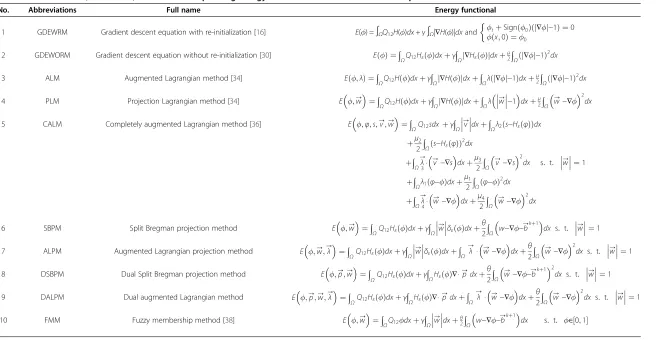
Table 1 Abbreviations, full names, and their corresponding energy functionals of all methods for comparison
No. Abbreviations Full name Energy functional
1 GDEWRM Gradient descent equation with re-initialization [16] E(ϕ) =
∫
ΩQ12H(ϕ)dx+γ∫
Ω|∇H(ϕ)|dxand ϕϕtðxþ;0SignÞ ¼ð Þϕϕ0ðj j−∇ϕ 1Þ ¼00
2 GDEWORM Gradient descent equation without re-initialization [30] Eð Þ ¼ϕ Z
ΩQ12Hεð Þϕdxþγ
Z
Ωj∇Hεð Þϕjdxþ
μ 2 Z
Ωðj j−∇ϕ 1Þ
2dx
3 ALM Augmented Lagrangian method [34] Eðϕ;λÞ ¼Z
ΩQ12Hð Þϕdxþγ Z
Ωj∇Hð Þϕjdxþ
Z
Ωλðj j−∇ϕ 1Þdxþ
μ 2 Z
Ωðj j−∇ϕ 1Þ
2dx
4 PLM Projection Lagrangian method [34] Eϕ;w→¼Z
ΩQ12Hð Þϕdxþγ
Z
Ωj∇Hð Þϕjdxþ
Z
Ωλ w →
−1
dxþμ2Z
Ω w →
−∇ϕ
2
dx
5 CALM Completely augmented Lagrangian method [36] Eϕ;φ;s;→v;w→¼Z
ΩQ12sdxþγ Z
Ω v →
dxþZ
Ωλ2ðs−Hεð ÞφÞdx
þμ22ZΩðs−Hεð ÞφÞ2dx
þZΩ→λ 3⋅ v
→ −∇s
dxþμ3
2 Z Ω v → −∇s 2 dx
þZΩλ1ðφ−ϕÞdxþμ1
2
Z
Ωðφ−ϕÞ
2 dx
þZΩ→λ4⋅w→−∇ϕdxþμ4
2 Z Ω w → −∇ϕ 2 dx
s: t: w→¼1
6 SBPM Split Bregman projection method Eϕ;w→¼Z
ΩQ12Hεð Þϕdxþγ
Z
Ω w →
δεð Þϕdxþθ2
Z
Ω w−∇ϕ−b →kþ1
dx s: t: w→¼1
7 ALPM Augmented Lagrangian projection method Eϕ;w→;→λ¼Z
ΩQ12Hεð Þϕdxþγ
Z
Ωw →
δεð ÞϕdxþZ
Ω λ →
⋅w→−∇ϕdxþθ
2 Z Ω w → −∇ϕ 2
dx s: t: w→¼1
8 DSBPM Dual Split Bregman projection method Eϕ;→p;w→¼Z
ΩQ12Hεð Þϕdxþγ
Z
ΩHεð Þ∇⋅ϕ p →dxþθ
2
Z
Ω w
→−∇ϕ−→bkþ1
2
dx s: t: w→¼1
9 DALPM Dual augmented Lagrangian method Eϕ;→p;w→;→λ¼Z
ΩQ12Hεð Þϕdxþγ
Z
ΩHεð Þ∇⋅ϕ p →
dxþZ
Ω λ →
⋅w→−∇ϕdxþθ
2 Z Ω w → −∇ϕ 2
dx s: t: w→¼1
10 FMM Fuzzy membership method [38] Eϕ;w→¼Z
ΩQ12ϕdxþγ Z
Ωw →
dxþθ2Z
Ω w−∇ϕ−b →kþ1
dx s: t: ϕ∈½0;1
Then, we project w→kþ1 as in Equation 27. Finally, the
Lagrangian multiplier→λ can be updated as the following:
λ
→
kþ1¼→λkþθw→kþ1− ∇ϕkþ1 ð42Þ
The advantages of the proposed four projection methods can be summarized as follows. (1): By introducing fewer auxiliary variables (i.e., two for SBPM, ALPM and three for DSBPM, DALPM) and considering the relation-ship between TV regularization term∫Ω|∇Hε(ϕ)|dxor its equivalent form∫Ω|∇ϕ|δε(ϕ)dxin Equation 22a and con-straint term |∇ϕ| = 1 in Equation 22b, we developed a very simple projection formula (27) in order to skillfully avoid expensive re-initialization process. (2): The proposed methods do not have many minimization and sub-maximization problems and penalty parameters due to the fewer auxiliary variables, so it is very easy and efficient to implement. (3): The final Euler-equations of proposed fast projection algorithms only include a simple Euler-Lagrange equation (24, 29, 35, 40) that can be solved via fast Gauss-Seidel iteration, a generalized soft thresholding formula in analytical form (26, 32), a fast iterative formula for dual variable (37), and a very simple projection formula (27). This technique can elegantly avoid computing the complex curvature and thus improve the efficiency. (4): All the proposed methods can preserve full LSF as a SDF precisely without a very large penalty parameter. This is due to the introduced Bregman iterative parameters (23a, 34) and Lagrangian multipliers (28a, 39) and the
projection computation, so a relatively large time step is allowed to be employed to speed up LSF evaluation as we will use semi-implicit gradient descent flow for (24, 29, 35, 40). (5): Even if the LSF is initialized as a piece-wise constant function, it can be corrected automatic-ally and precisely due to the projection computation. In conclusion, our proposed four projection methods will have both higher computational efficiency and better SDF fidelity, which can be validated in the next experi-mental Section.
4. Numerical experiments
In this section, we present some numerical experiments to compare the effectiveness and efficiency of our methods (i.e., SBPM, ALPM, DSBPM, and DALPM) with five previous ones (i.e., GDEWRM, GDEWORM, ALM, PLM, and CALM). In addition, we also compare the proposed four methods with the fast algorithm proposed in [38] for Chan-vese model under VLFM framework [20], which is named in this paper as fuzzy membership method (FMM). Therefore, there are totally ten algo-rithms involved in this paper. In order to make it easier to assess the exact differences between these models, we list the abbreviations of all methods, their full name, and corresponding energy functionals in Table 1.
In order to make the comparisons fair among different methods, we solve the PDEs in Equations 15, 17, 18, 19, 24, 29, 35, and 40 by semi-implicit difference scheme based on their gradient descent equations. As for FMM, we here adopt the method proposed in [38]. For CALM, we use the Gauss-Seidel fixed point iteration for solving
the LSF ϕ instead of fast Fourier transformation (FFT) for fair comparison with others. The initial LSF ϕ0 is initialized as a same piecewise constant function for all the methods except initializing a SDF for GDEWRM. Equation 8 is solved by using the first order upwind scheme in every five iterations. In experiments 1 and 2, we set a one-step iteration for inside loop computation of ϕ for all the methods. However, ten-step iterations for ϕ in experiment 3 are required to achieve the final 3D SDFs fast. The parameter γ is usually formatted by γ=η× 2552, η∈ (0,1). We set the spatial step h= 1 and α1=α2= 1, τ= 0.125, ε= 3. The stopping criterion is
based on the relative energy error formula |Ek + 1−Ek|/ Ek≤ξ, whereξis a small prescribed tolerance and here we set 10−3in all numerical experiments. All experiments are performed using Matlab 2010b on a Windows 7 platform with an Intel Core 2 Duo CPU at 2.33GHz and 2GB memory.
4.1 Experiment 1
In this experiment, we aim to compare the proposed four methods with the fast algorithm FMM. As FMM uses binary or label functions and continuous convex re-laxation technique, it is very robust for initialization and fast and guaranteed to find a global minimizer. Our methods and FMM are applied to segment two medical images. One is MRI image of brain in the first row of Figure 1, and the other is CT image of vessel in the second
row. The five methods are initialized with the same piecewise constant function (0 and 1). Here, we draw the red contours to represent their initial contours in the first column of Figure 1. Columns 2, 3, 4, 5, and 6 are the final segmentation results (i.e., green contours) by SBPM, ALPM, DSBPM, DALPM, and FMM, respect-ively. In order to make detailed comparisons, we crop a part of region indicated by the yellow rectangle in Figure 1 and enlarge them in Figure 2 where the first four columns are the results by the proposed four methods, respectively, and the last column is by FMM. One can observe from Figures 1 and 2 that the white matter in the brain and the vessel are extracted correctly and perfectly by the four methods. However, the results by FMM are less desirable. This can be clearly observed in column 5 of Figure 2, where some undesirable results of structure segmentation are marked with blue circles. However, we cannot tell easily some major differences among those segmentation results by all the four proposed methods. Further, fewer iterations and fast computational time shown in Table 2 demonstrate that the four methods are comparatively efficient as the fast FMM. In fact, the SBPM, ALPM, DSBPM, and DALPM are just different iterative schemes to solve the same system. The authors in [28] have proven their equiva-lence for the TV model. The segmentation results in Figure 1 and iterations and CPU times in Table 2 demonstrate consistency with their conclusion.
Figure 2Zoom in small sub-regions of images in Figure 1 for detail comparisons. (a-j)The enlarged region of panels b to l of Figure 1, respectively.
Table 2 Comparisons of iterations and computation time among our proposed fast methods
Image (size) SBPM ALPM DSBPM DALPM FMM
Iterations CPU
time (s)
Iterations CPU
time (s)
Iterations CPU
time (s)
Iterations CPU
time (s)
Iterations CPU
time (s)
Brain (123 × 155) 19 0.327 19 0.331 20 0.308 20 0.325 22 0.326
Vessel (95 × 152) 23 0.313 22 0.306 22 0.309 22 0.303 24 0.329
4.2 Experiment 2
In this experiment, we will compare the efficiency of our methods with that of GDEWRM, GDEWORM, ALM, PLM, and CALM. All nine methods are run on four real and synthetic images including squirrel, ultrasound baby, leaf, and synthetic noise number images, respectively. In the first column of Figure 3, we initialize piecewise constant function (0 and 1) for all methods except
GDEWRM, which is initialized with a SDF. Columns 2, 3, 4, 5, and 6 of Figure 3 are the results by GDEWRM, GDEWORM, ALM, PLM, and CALM respectively. In the last column of Figure 3, we only present the final segmentation result of squirrel, ultrasound baby, leaf, and number image by SBPM, ALPM, DSBPM, and DALPM respectively, because the visual effect and com-putational efficiency for all the four proposed methods Figure 3Comparisons of our different projection methods with previous five ones.To segment a squirrel image, an ultrasound baby image, a leaf image, and a synthetic noise number image.(a, h, o, v)Original image with initial green contour.(b, i, p, w)Results by GDEWRM.
(c, j, q, w)Results by GDEWORM.(d, k, i, y)Results by ALM.(e, l, s, z)Results by PLM.(f, m, t, I)Results by CALM.(g, n, u, II)Results by our projection methods (from top to bottom is SBPM, ALPM, DSBPM, and DALPM, respectively).
Table 3 Comparison of iterations and computation time using different segmentation methods
Methods Iterations CPU time (s)
Squirrel Ultrasound baby Leaf Numbers Squirrel Ultrasound baby Leaf Number
(155 × 122) (180 × 175) (128 × 87) (128 × 127) (155 × 112) (180 × 175) (128 × 87) (128 × 127)
GDEWRM 165 372 98 100 4.296 12.769 3.070 4.230
GDEWORM 166 108 85 38 2.543 4.905 1.978 1.666
ALM 46 100 64 31 1.243 3.803 1.163 0.945
PLM 109 92 69 34 1.211 2.813 0.738 0.596
CALM 32 39 62 26 0.696 1.365 0.685 0.498
SBPM 24 28 28 14 0.389 0.723 0.256 0.202
ALPM 23 26 27 15 0.372 0.707 0.237 0.212
DSBPM 24 25 29 13 0.381 0.692 0.258 0.192
are very similar on these images. From Figure 3, we can see that all the methods do a relatively good performance for segmenting both real and noise synthetic images. However, compared with other methods, all the four pro-posed methods perform better, which can be observed in the last column of Figure 3. In addition, we record total it-erations and computation time of all nine methods for segmenting these images in Table 3. In order to make the experimental data in Table 3 meaningful, we draw Figure 4 to illustrate the differences regarding iterations and com-putation time. Figure 4a,b,c,d shows the total iterations with bar chart of all nine methods for segmenting squirrel, ultrasound baby, leaf, and number images, respectively, and Figure 4e,f,g,h draws the total CPU time for segment-ing these images. Accordsegment-ing to Figure 4e,f,g,h, the compu-tational time of the nine methods can be clearly ranked in the following order: SBPM≈ALPM≈DSBPM≈DALPM< CALM<PLM<ALM<GDEWORM<GDEWRM. The reason leading to this rank can be justified as follows. (1) All the methods compute faster than the GDEWRM due to its expensive re-initialization process. (2) Among these methods without re-initialization, ALM, PLM, and CALM are running faster than GDEWORM. For GDEWORM, the CFL condition limits its time step so that it cannot be fast, while ALM improves convergence rate by introdu-cing Lagrange multiplierλ. PLM uses Lagrangian method and variable splitting technique to enhance the evolution
speed, so PLM is faster than ALM. However, both ALM and PLM are limited by CFL condition and their speed is slowed. CALM introduces many scalar or vector auxiliary variables and Lagrangian multipliers to make each sub-problem very simple as well as can avoid CFL condition, so it computes faster than ALM and PLM. (3) All the pro-posed methods can achieve the best efficiency and satis-factory segmentation results because the nonlinear curvature is replaced by the linear Laplace operator in Equations 24 and 29 or the dual divergence operator in Equations 35 and 40 as simple projection technique (27)
(a) Iterations of all methods (b) Iterations of all methods for (c) Iterations of all methods (d) Iterations of all methods for squirrel segmentation ultrasound baby segmentation for leaf segmentation for number segmentation
(e) CPU time of all methods (f) CPU time of all methods for (g) CPU time of all methods (h) CPU time of all methods for squirrel segmentation ultrasound baby segmentation for leaf segmentation for number segmentation
Figure 4Graph Expression of iterations and CPU time of all the methods in Table 3. (a),(b),(c),and(d)Iterations of all methods for segmenting squirrel, ultrasound baby, leaf and synthetic noise number images respectively.(e),(f),(g),and(h)Record of their CPU time.
Table 4 Comparison of iterations, computation time, and SDF fidelity using different segmentation methods
Methods Iterations CUP time (s) SDF fidelity value
GDEWRM 200 77.236 0.0385
GDEWORM 2000 224.094 0.4407
ALM 600 69.624 1.9005
PLM 500 46.644 0.0441
CALM 200 18.545 0.0259
SBPM 50 5.296 0.0149
ALPM 50 5.197 0.0149
DSBPM 50 4.924 0.0153
DALPM 50 5.213 0.0153
is used. In comparison with CALM, our projection methods have fewer sub-problems, so it is very efficient. In addition, by introducing the Bregman iterative parameters (23a, 34) and Lagrangian multipliers (28a, 39), a relatively large time step can be used to speed up LSF evaluation. Therefore, our methods compute faster than CALM and their efficiency ranks first. (4) The proposed four fast methods (i.e., SBPM, ALPM, DSBPM, and DALPM) are actually equivalent, which is validated in [25]. Therefore, these projection methods have very similar computation speed.
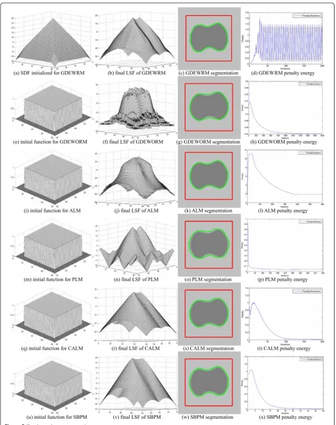
4.3 Experiment 3
In this experiment, we aim to compare SDF fidelity pro-duced by our four methods and the other five. We seg-ment a synthetic image (100 × 100) to obtain the SDF fidelity value in Table 4 as explained below. The first col-umn of Figure 5 is the initial LSFs for all the methods. As there is no constraint of LSF as a SDF in GDEWRM, panel a is initialized as a SDF for this method. However, if it is initialized as a piecewise constant function, the LSF will be far away from SDF during the contour evalu-ation, even though the re-initialization process may be not able to pull LSF back to SDF. In this case, the com-parisons of SDF preservation with other methods with-out re-initialization are not very fair. Based on the above observation, Figure 5e,i,m,q,u is initialized as the same piecewise constant function for GDEWORM, ALM, PLM, CALM, and SBPM, respectively. As all of our four projection methods achieve almost the same results, here, we only give the experimental data for SBPM in the last row of Figure 5. In the second column of
Figure 5b,f,j,n,r,v are the final 3D LSFs of GDEWRM, GDEWORM, ALM, PLM, CALM, and SBPM, respect-ively. In the third column of Figure 5c,g,k,o,s,w are the same initial contours marked by red rectangle and the final segmentation results marked by green contours of above methods. In the last column, we draw the plots of mean value of penalty energy ∫ Ω(|∇ϕ|−1)2dx by the above corresponding methods, which is used to measure the closeness between LSF and SDF. We denote SDF fi-delity value as mean value in the last iteration for every method. The smaller this value is, the closer the LSF and SDF will be. We also put all these results in Table 4 for easy comparison.
Note that the final LSF of GDEWRM in Figure 5b is very close to SDF, which is validated by its very small SDF fidelity value (0.0385) in Table 4. However, the final green segmentation contour in Figure 5c shows that the zero level set of Figure 5b by this GDEWRM shrinks and cannot reach the exact location of the object. In fact, in order to obtain Figure 5b, this GDEWRM needs 300 re-initialization iterations after every five-step iter-ation of LSF evolution. So it is very expensive (total 77.236 s reported in Table 4), and this re-initialization leads to large jumps in its penalty energy plots in Figure 5d. For GDEWORM and PLM, their experimen-tal results are displayed in the second and fourth row, respectively. Although their final SDF fidelity values are close to zero (i.e., 0.4407 for GDEWORM and 0.0441 for PLM), their final SDFs as shown in Figure 5f,n are not preserved nicely. Moreover, due to CFL condition, we need to choose a very small time step 10−4 and a very large penalty parameter 2 × 10⁴ for GDEWORM and (See figure on previous page.)
Figure 5SDF fidelity comparisons of our projection methods with previous methods. (a, e, i, m, q, u)Initial LSFs.(b, f, j, n, r, v)Final LSFs.(c, g, k, o, s, w)Initial contours marked by red rectangle and final segmentation results indicated by green contours.(d, h, l, p, t, x)Mean value of penalty energy plots∫Ω(|∇ϕ|−1)2dx(closeness measure between LSF and SDF).
(a) Iterations of all methods for a synthetic (b) CPU time of all methods for a synthetic (c) SDF fidelity value of all methods for a image segmentation in Fig 5 image segmentation in Fig 5 synthetic image segmentation in Fig 5
Figure 6Graph expression of iterations and CPU time and SDF fidelity of all the methods in Table 4. (a), (b),and(c)Record iterations, CPU time, and SDF fidelity value of all methods, respectively.
PLM, respectively. This selection is aimed to guarantee the closeness between the LSF and SDF and stability of LSF evolution, but this leads to a large number of total iterations (i.e., respective 2,000 and 500). As we analyzed in experiment 2, PLM adopts variable splitting technique and therefore its total computation time and iterations are much less than GDEWORM. As large penalty pa-rameters are employed in PLM and GDEWORM, we find that the final green contours by these two methods cannot segment the object precisely. For ALM, it im-proves convergence rate by introducing Lagrange multi-plierλ so that we can choose a slightly larger time step 10−2 and a relatively smaller penalty parameter 10−1to evolve the LSF. However, we conducted a great number of experiments for this method and note that it is very sensitive to parameters selection. Also, its final SDF fi-delity value is always the largest among all the methods. This may be due to the fact that the introduced Lagrangian multiplier in ALM breaks the CFL condition. The fourth row of Figure 5 that demonstrates CALM is able to achieve a better 3D SDF (shown in Figure 5f) and a smaller SDF fidelity value (0.0259 shown in Table 4) than those by other methods except our methods. The compu-tation speed of this method has been improved to a great extent as observed in Table 4 and Figure 5t. The last row of Figure 5 presents the experimental data by our pro-posed SBPM. Here, we emphasize that the other three proposed methods can achieve almost that same SDF and efficiency as SBPM. From Figure 5v, the final 3D LSF is perfectly preserved as SDF fidelity value is only 0.0149, the smallest one among all the methods in Table 4. Most im-pressively, we find that penalty parameter 10 can be large enough to penalize accurately the full LSF as SDF due to the introduced Lagrangian multiplier, Bregman iterative parameter, and the precise projection computation. In this case, a relatively large time 10−2can be employed to speed up LSF evolution as shown in Figure 5x. In addition, even if the LSF is initialized as a piecewise constant function for SBPM, it can be corrected automatically and precisely due to the projection formula (27).
Lastly, we present Figure 6 that includes three bar graphs which correspond to iterations, CUP time, and SDF fidelity value in Table 4, respectively. However, Figure 6b shows that the slowest method is GDEWORM rather than GDEWRM, which is inconsistent with the conclusion in experiment 2. In fact, the time step in GDEWRM is set 10−2, 100 times larger than that set for GDEWORM. We find that this time step together with 300 re-initialization iterations would not broke the sta-bility of LSF evolution and simultaneously is able to achieve a very desirable SDF. In contrast, for the pur-pose of preserving distance feature, we should choose a very large penalty parameter for GDEWORM, which limits the speed of LSF evolution. Therefore, in this
experiment, on the premise of preserving distance feature, the GDEWRM is faster than GDEWORM. From Figure 6c, the ability of SDF fidelity can be ranked as SBPM≈ ALPM≈DSBPM≈DALPM>CALM>GDEWORM> PLM>GDEWRM>ALM.In conclusion, this experiment validates that the four projection methods perform excel-lently in both accuracy and speed of preserving SDF.
5. Conclusions
In this paper, by investigating the relationship between the L1-based TV regularizer term of Chan-Vese model and the constraint on LSF and introducing some auxil-iary variables, we design fast split Bregman projection method (SBPM), augmented Lagrangian projection method (ALPM), dual split Bregman projection method (DSBPM), and dual augmented Lagrangian projection method (DALPM). All these methods can skillfully avoid the expensive re-initialization process and simplify compu-tation of curvatures. In our methods, there are fewer sub-problems and penalty parameters, so they can be solved ef-ficiently. Moreover, the full LSF can be preserved as a SDF precisely without a very large penalty parameter so that a relatively large time step can be used to speed up LSF evaluation. In addition, even if the LSF is initialized as a piecewise constant function, it can be corrected automatic-ally and accurately due to analytical projection computa-tion. Simulation experiments have validated the efficiency and performance of proposed methods in terms of compu-tational cost and SDF fidelity.
Abbreviations
ALM:augmented Lagrangian method; ALPM: augmented Lagrangian projection method; CALM: completely augmented Lagrangian method; CFL: Courant-Friedrichs-Lewy; DALPM: dual augmented Lagrangian method; DSBPM: dual split Bregman projection method; FFT: fast Fourier
transformation; FMM: fuzzy membership method; GDEWORM: gradient descent equation without re-initialization; GDEWRM: gradient descent equation with re-initialization; KKT: Karush-Kuhn-Tucker; LSF: level set function; LSM: level set method; PDEs: partial differential equations; PLM: projection Lagrangian method; SBPM: split Bregman projection method; SDF: sign distance function; TV: total variation; VLFM: variational label function method; VLSM: variational level set method.
Competing interests
The authors declare that they have no competing interests.
Acknowledgments
This work was supported by the National Natural Science Foundation of China (nos.61305045, 61170106, and 61303079), National‘Twelfth Five-Year’ Development Plan of Science and Technology (no.2013BAI01B03), and Qingdao Science and Technology Development Project (no. 13-1-4-190-jch).
Received: 10 April 2013 Accepted: 7 January 2014 Published: 27 January 2014
References
1. JM Morel, S Solimini,Variational Methods in Image Segmentation(Birkhauser, Boston, 1994)
3. S Osher, N Paragios,Geometric Level Set Methods in Imaging, Vision, and Graphics(Springer, Heidelberg, 2003)
4. A Mitiche, IB Ayed,Variational and Level Set Methods in Image Segmentation
(Springer, Heidelberg, 2010)
5. M Kass, A Witkin, D Terzopoulos, Snakes: active contour models. Int. J. Comput. Vis.4(1), 321–331 (1987)
6. D Mumford, J Shah, Optimal approximations by piecewise smooth functions and associated variational problems. Commun. Pure Appl. Math. 42(5), 577–685 (1989)
7. G Aubert, M Barlaud, O Faugeras, S Jehan-Besson, Image segmentation using active contours: calculus of variations or shape gradient. SIAM J. Appl. Math.63(6), 2128–2154 (2003)
8. G Aubert, M Barlaud, S Duffner, A Herbulot, S Jehan-Besson, Segmentation of vectorial image features using shape gradients and information measures. J. Math. Imaging Vis.25(3), 365–386 (2006)
9. G Aubert, M Barlaud, E Debreuve, M Gastaud, Using the shape gradient for active contour segmentation: from the continuous to the discrete formulation. J. Math. Imaging Vis.28(1), 47–66 (2007)
10. S Osher, JA Sethian, Fronts propagating with curvature-dependent speed: algorithms based on Hamilton-Jacobi formulations. J. Comput. Phys. 79(1), 12–49 (1988)
11. L Ambrosio, VM Tortorelli, Approximation of functionals depending on jumps by elliptic functionals via gamma-convergence. Commun. Pur. Appl. Math.43(8), 999–1036 (1990)
12. S Esedoglu, YH Tsai, Threshold dynamics for the piecewise constant Mumford-Shah functional. J. Comput. Phys.211(1), 367–384 (2006) 13. YM Jung, SH Kang, JH Shen, Multiphase image segmentation by
Modica-Mortola phase transition. SIAM J. Appl. Math.67(5), 1213–1232 (2007) 14. I Posirca, YM Chen, CZ Barcelos, A new stochastic variational PDE model for
soft Mumford-Shah segmentation. J. Math. Anal. Appl.384(1), 104–114 (2011)
15. HK Zhao, TF Chan, B Merriman, S Osher, A variational level set approach to multiphase motion. J. Comput. Phys.127(1), 179–195 (1996)
16. TF Chan, LA Vese, Active contours without edges. IEEE Trans. image process. 10(2), 266–277 (2001)
17. LA Vese, TF Chan, A multiphase level set framework for image segmentation using the Mumford and Shah model. Int. J. Comput. Vis. 50(3), 271–293 (2002)
18. C Samson, L Blanc-Feraud, G Aubert, A level set model for image classification. Int. J. Comput. Vis.40(3), 187–197 (2000)
19. G Chung, LA Vese, Energy minimization based segmentation and denoising using a multilayer level set approach. LNCS, Springer-Verlang3757, 439–455 (2005)
20. X Bresson, S Esedoglu, P Vandergheynst, JP Thiran, S Osher, Fast global minimization of the active contour/snake model. J. Math. Imaging Vis. 28(2), 151–167 (2007)
21. J Lie, M Lysaker, XC Tai, A binary level set model and some applications to Mumford-Shah image segmentation. IEEE Trans. Image process. 15(5), 1171–1181 (2006)
22. J Lie, M Lysaker, XC Tai, A variant of the level set method and applications to image segmentation. Math. Comput.75(255), 1155–1174 (2006) 23. F Li, K Michael, T Zeng, C Shen, A multiphase image segmentation method
based on fuzzy region competition. SIAM J. Imaging Sci.3(3), 277–299 (2010)
24. T Goldstein, S Osher, The split Bregman method for L1 regularized problems. SIAM J. Imaging Sci.2(2), 323–343 (2009)
25. T Goldstein, X Bresson, S Osher, Geometric applications of the split Bregman method: segmentation and surface reconstruction. J. Sci. Comput.45(1–3), 272–293 (2009)
26. A Chambolle, An algorithm for total variation minimization and applications. J. Math. Imaging Vis.20(1), 89–97 (2004)
27. ES Brown, TF Chan, X Bresson, Completely convex formulation of the Chan-Vese image segmentation model. Int. J. Comput. Vis.98(1), 103–121 (2012) 28. C Wu, XC Tai, Augmented Lagrangian method, dual methods, and split
Bregman iteration for ROF, vectorial TV, and high order models. SIAM J. Imaging Sci.3(3), 300–339 (2010)
29. YHR Tsai, LT Cheng, S Osher, HK Zhao, Fast sweeping algorithms for a class of Hamilton-Jacobi equations. SIAM J. Numer. Anal.41(2), 673–694 (2003) 30. C Li, C Xu, C Gui, MD Fox, Level set evolution without re-initialization: a new
variational formulation, inProceedings of IEEE conference on Computer Vision and Pattern Recognition (CVPR), 1st edn. San Diego20–25, 430–436 (2005)
31. D Adalsteinsson, JA Sethian, The fast construction of extension velocities in level set methods. J. Comput. Phys.148(1), 2–22 (1999)
32. D Peng, B Merriman, S Osher, HK Zhao, M Kang, A PDE-based fast local level set method. J. Comput. Phys.155(2), 410–438 (1999)
33. M Sussman, E Fatemi, An efficient, interface preserving level set re-distancing algorithm and its application to interfacial incompressible fluid flow. SIAM J. Sci. Comput.20(4), 1165–1191 (1999)
34. C Liu, F Dong, S Zhu, D Kong, K Liu, New variational formulations for level set evolution without reinitialization with applications to image segmentation. J. Math. Imaging Vis41(3), 194–209 (2011)
35. R Courant, K Friedrichs, H Lewy, On the partial difference equations of mathematical physics. IBM J11(2), 215–234 (1967)
36. V Estellers, D Zosso, R Lai, S Osher, JP Thiran, X Bresson, An efficient algorithm for level set method preserving distance function. IEEE Trans. Image Process.21(12), 4722–4734 (2012)
37. C Liu, Z Pan, J Duan, New algorithm for level set evolution without re-initialization and its application to variational image segmentation. J Software8(9), 2305–2312 (2013)
38. X Bresson, A Short Guide on a Fast Global Minimization Algorithm for Active Contour Models (Online). https://googledrive.com/host/
0B3BTLeCYLunCc1o4YzV1Ui1SeVE/codes_files/xbresson_2009_short_guide_ global_active_contours.pdf. Accessed 22 Apr 2009
doi:10.1186/1687-5281-2014-7
Cite this article as:Duanet al.:Some fast projection methods based on
Chan-Vese model for image segmentation.EURASIP Journal on Image and
Video Processing20142014:7.
Submit your manuscript to a
journal and benefi t from:
7Convenient online submission
7Rigorous peer review
7Immediate publication on acceptance
7Open access: articles freely available online
7High visibility within the fi eld
7Retaining the copyright to your article