R E S E A R C H
Open Access
Vehicle classification framework: a comparative
study
Amol Ambardekar
*, Mircea Nicolescu, George Bebis and Monica Nicolescu
Abstract
Video surveillance has significant application prospects such as security, law enforcement, and traffic monitoring. Visual traffic surveillance using computer vision techniques can be non-invasive, cost effective, and automated. Detecting and recognizing the objects in a video is an important part of many video surveillance systems which can help in tracking of the detected objects and gathering important information. In case of traffic video surveillance, vehicle detection and classification is important as it can help in traffic control and gathering of traffic statistics that can be used in intelligent transportation systems. Vehicle classification poses a difficult problem as vehicles have high intra-class variation and relatively low inter-class variation. In this work, we investigate five different object recognition techniques: PCA + DFVS, PCA + DIVS, PCA + SVM, LDA, and constellation-based modeling applied to the problem of vehicle classification. We also compare them with the state-of-the-art techniques in vehicle classification. In case of the PCA-based approaches, we extend face detection using a PCA approach for the problem of vehicle classification to carry out multi-class classification. We also implement constellation model-based approach that uses the dense representation of scale-invariant feature transform (SIFT) features as presented in the work of Ma and Grimson (Edge-based rich representation for vehicle classification. Paper presented at the international conference on computer vision, 2006, pp. 1185–1192) with slight modification. We consider three classes: sedans, vans, and taxis, and record classification accuracy as high as 99.25% in case ofcarsvsvansand 97.57% in case ofsedansvstaxis. We also present a fusion approach that uses both PCA + DFVS and PCA + DIVS and achieves a classification accuracy of 96.42% in case ofsedansvsvansvstaxis.
Keywords:Computer vision; Video surveillance; Pattern recognition; Traffic monitoring; Vehicle classification; Machine vision and scene understanding; Image processing
MSC:68T10; 68T45; 68U10
1 Introduction
Visual traffic surveillance has attracted significant interest in computer vision, because of its significant application prospects. Efficient and robust localization of vehicles from an image sequence (video) can lead to semantic results, such as‘Vehicle No. 3 stopped,’ ‘Vehicle No. 4 is moving faster than Vehicle No. 6.’ However, such infor-mation can be more relevant if we not only can detect ve-hicles but also can classify them. Information such as gap, headway, stopped-vehicle detection, speeding vehicle, and class of a vehicle can be useful for intelligent transpor-tation systems [1]. Monitoring vital assets using video surveillance has increased in recent years. The class of a detected vehicle can supply important information
that can be used to make sure that certain types of vehi-cles do not appear in certain areas under surveillance. Multi-camera systems such as the one used in [2] can benefit immensely if the information regarding the classes of vehicles is available, as vehicle classification can be used in matching objects detected in non-overlapping field of views from different cameras.
Object detection and tracking has achieved good accur-acy in recent years. However, the same cannot be said about object classification. Object recognition in case of still images has the problem of dealing with the clutter in the scene and a large number of classes. Object recognition in video sequences has the benefit of using background segmentation to remove clutter [3]. However, images obtained from video surveillance cameras are generally of low resolution, and in case of traffic video surveillance, * Correspondence:[email protected]
University of Nevada, 1664 N Virginia St., Reno, NV 89557, USA
the vehicles cover very small areas of these images, making the classification problem challenging. Vehicle classes such as carsand vansare difficult to differentiate as they have similar sizes. Therefore, classification techniques that use global features such as size and shape of the detected blob do not yield satisfactory results.
For this work, we consider three vehicle classes: cars, vans, and taxis. Classes like bus, semi, and motorcycle were not included because they are relatively easy to classify based on their size. We considered three differ-ent scenarios:carsvsvans,sedansvstaxis, andsedans vsvans vstaxis. Taxis and sedans are disjoint subsets of class cars. Therefore, results ofsedans vstaxiswill demonstrate the relevance of our approach when inter-class variability is low. For the purpose of this paper, we used a dataset provided in [4].
In [3], Ambardekar et al. presented a comprehensive traffic surveillance system that can detect, track, and classify the vehicles using a 3D model-based approach. The classification using the 3D model-based approach requires camera parameters and orientation of a vehicle which can be calculated using tracking results. When ve-hicle orientation information is available, the methods presented in this paper can be used in a traffic surveillance system such as [3] to improve the vehicle classification accuracy.
In this work, we present five different vehicle classifi-cation techniques that can be used in combination with a consideration to the requirements of the scenario and do not require camera calibration. The two main contri-butions of our work are the following: (1) We present sev-eral approaches (PCA + DFVS, PCA + DIVS, PCA + SVM, LDA, and constellation model) and improvements over the published results that used state-of-the-art techniques. (2) We perform a comparative study of these and other approaches in the literature for the purpose of vehicle classification.
There are similarities between the problem of face de-tection and vehicle recognition especially in the typical size of an image sample under consideration. In face de-tection, the problem is finding a face from non-face image samples. However, in case of vehicles, we have multiple classes, and we want to differentiate between them. Turk and Pentland used PCA to form eigenfaces that can reli-ably recognize faces [5]. We extend the face detection based on PCA and implement three different techniques: PCA + DFVS, PCA + DIVS, and PCA + SVM. In these ap-proaches, we create a principal component space (PCS) using PCA which we call vehicle space. In case of PCA + DFVS, the decision is made by finding the distance from a separate vehicle space for each class, and therefore, it is named distance from vehicle space (DFVS). On the other hand, PCA + DIVS predicts the class of a test image after projecting a test image onto a combined vehicle space,
and distance from each class is calculated in vehicle space and hence named distance in vehicle space (DIVS). We achieved an overall accuracy as high as 95.85% in case of sedansvsvansvstaxisusing PCA + DFVS. In the difficult case of sedans vs taxis, we achieved a 97.57% accuracy using PCA + DFVS which is higher than any published results using this dataset [6,7]. PCA + DIVS yielded 99.25% accuracy in case of cars vs vans. Our results match or surpass the results in all the cases considered in [4,8]. PCA depends upon most expressive features (MEFs) that can be different from most discriminant features (MDFs) [9]; therefore, we also implement LDA that relies on MDFs. We observed that PCA + DIVS approach works better when the classes have more inter-class vari-ation, e.g.,carsvs vans, and PCA + DFVS seems to work better even in the difficult case of sedans vs taxis when inter-class variation is low. Therefore, we devised a new fusion approach that combines the benefits of both the approaches to classify sedans vs vans vs taxis, and were able to achieve classification accuracy of 96.42%.
Constellation models [10,11] have been shown to be able to learn to recognize multiple objects using a training set of just a few examples. In [4], Ma and Grimson used a constellation model with mean-shift clustering of scale-invariant feature transform (SIFT) features to classify vehi-cles. However, the mean-shift clustering is considerably slow. In our implementation, we used K-means clustering. We also use an expectation maximization algorithm that considers up to 6 Gaussians and choose the number of Gaussians that maximizes the maximum likelihood for training data. We achieved similar accuracy with consid-erably less computation complexity compared to results achieved in [4]. In [4], Ma and Grimson dealt with only a two-class classification problem. We extend the approach by performing classification in the three class case ofsedans vsvansvstaxis.
The rest of the paper is organized as follows: Section 2 discusses previous work. Section 3 gives details about the techniques compared in this paper, and Section 4 describes and compares the results obtained. Section 5 discusses the conclusions and future work.
2 Existing video annotation and retrieval systems Object classification in general is a challenging field. Vehicle classification poses another challenge as inter-class variability is relatively smaller compared to intra-class variability. The approaches for vehicle classification can be broadly classified into four categories.
2.1 3D model-based approaches
using background subtraction. Edges were detected using either the Sobel edge detector or the Canny edge detector. 3D wireframes of the models in the database are projected onto the image, and the best match is found based on the best matching pixel position [14], or mathematical morph-ology to match the model to the edge points [3]. All the models are subjected to the matching process, and the one with the highest matching score (i.e., lowest matching error) is selected as the model. These methods require camera parameters to be calibrated so that a 3D wireframe can be projected onto an image. They also need orienta-tion of the vehicles which can be retrieved from optical flow calculation.
2.2 Global feature-based approaches
Gupteet al.[15] proposed a system for vehicle detection and classification. They classified the tracked vehicles into two categories: cars and non-cars. The classification is based on vehicle dimensions, where they compute the length and height of a vehicle and use them to distinguish cars from non-cars [15]. Avely et al. [16] used a similar approach, where the vehicles are classified on the basis of length using an uncalibrated camera. However, this method also classifies the vehicles into two coarse groups: short vehicles and long vehicles. In order to achieve a finer-level classification of vehicles, a more refined method needs to be devised that can detect and model the invariant characteristics for each vehicle category considered.
2.3 PCA-based approaches
Chunrui and Siyal developed a new segmentation tech-nique for the classification of moving vehicles [17]. They used simple correlation to get the desired match. The results shown in the paper are for the lateral view of the vehicles, and no quantitative results were given. Towards this goal, a method is developed by Zhanget al.[18]. In their work, they used a PCA-based vehicle classification framework. They implemented two classification algo-rithms: eigenvehicle and PCA-SVM to classify vehicle objects into trucks, passenger cars, vans, and pickups. These two methods exploit the distinguishing power of principal component analysis (PCA) at different granular-ities with different learning mechanisms. Eigenvehicle ap-proach used in [18] is similar to the proposed apap-proach PCA + DIVS. However, we use distance from mean image in PCA space instead of finding distance from each image from each class as done in [18]. The performance of such algorithms also depends on the accuracy of vehicle normalization.
2.4 Local feature-based approaches
Local features have certain advantages over using global features as they are better suited to handle partial
occlusion. In traffic surveillance, if the intersection moni-toring is desired, then overlapping of passing vehicles will result in partial occlusion and errors in extracting ROIs. SIFT [19] has shown to outperform other local features in terms of repeatability [20].
Ma and Grimson developed a vehicle classification approach using modified SIFT descriptors [4]. They used SIFT features to train the constellation models that were used to classify the vehicles. They considered two cases:carsvsvansandsedansvstaxis. They reported good results for the difficult case of classifyingsedans vs taxis. However, they do not report combined classification results for sedans vs vans vs taxis that will show the scalability of the approach. We used the same dataset provided by them. We implemented constellation model-based approach that differs slightly from [4], but we were able to achieve similar accuracy with better computational complexity.
2.5 Other approaches
Koch and Malone [21] used infrared video sequences and a multinomial pattern-matching algorithm [22] to match the signature to a database of learned signatures to do classification. They started with a single-look approach where they extract a signature consisting of a histogram of gradient orientations from a set of regions covering the moving object. They also implemented a multi-look fusion approach for improving the performance of a single-look system. They used the sequential probability ratio test to combine the match scores of multiple signatures from a single tracked object. Huang and Liao [23] used hierarchical coarse classification and fine classification. Ji et al.used a partial Gabor filter approach [24]. In [8], Wijnhoven and de With presented a patch-based approach that uses Gabor-filtered versions of the input images at several scales. The feature vectors were used to train a SVM classifier which was able to produce results better than those presented in [4] incarsvsvanscase. However, this approach is global feature based; therefore, it is not best suited for cases with partial occlusion. Recently, Buch et al.presented a traffic video surveillance system which employs motion 3D extended histogram of oriented gra-dients (3DHOG) to classify road users [6].
3 Classification framework
model is a part-based model, it can perform well even in the presence of partial occlusion.
3.1 Eigenvehicle approach (PCA + DFVS)
The images in the dataset have different sizes and there-fore are not suitable for PCA directly. We normalize all the images to average width and height (74 × 43). In [5], PCA was used for single-class classification (i.e., face). We use it for up to three classes at the same time and therefore extend the approach by creating a separate PCS or vehicle space for each class. We define each eigenspace as eigenvehicle [18].
3.1.1 Training for eigenvehicles
For creating the principal component space for each class, i.e., creating eigenvehicle for each class, we normalize the images such that the width and height of all the images are the same. Since each sample image is a 2-D image,Ai∈
Rm×n, we create a vector from an image by concatenating rows to create a column vectorA′i∈R1 ×mn. We consider
k= 50 images for each class; then, we have a matrix of k columnsA′= [A′1A′2A′3…A′k] that represents the set of
training samples. The length of each column is m×n. Then, we can compute the mean vectorμas below:
μ¼1 k
Xk i¼1A
0
i: ð1Þ
Letσi=A′i−μ, andσ= [σ1,σ2,σ3,…σk]. The covariance
matrix ofA′is
C¼1 k
Xk i¼1σiσ
T
i ¼σσT ð2Þ
The eigenvectors of C are the principal components. The eigenvectors associated with the largest eigenvalues correspond to the dimensions in the space where the
data has the largest variance. In our training set, the size ofC ismn×mn(3,182 × 3,182), which is not feasible to compute principal components. In [5], Turk and Pentland proposed a solution to this problem, where they find the eigenvectors and eigenvalues ofσTσ, instead of σσT. Sup-pose vi is an eigenvector ofσTσ, and λi is the associated
eigenvalue. Then,
σTσv
i¼λivi → yields
σσTσv
i¼λiσvi ð3Þ
The above deduction shows thatσviis an eigenvector of
σσT. This technique reduces the computation complexity
since the dimension ofσTσis onlyk×k(50 × 50). We are able to extract topkprincipal components ofσσTby the following equation:
ui¼σvi ð4Þ
The eigenvectors corresponding to the biggest eigenvalue represent the most dominant dimensions or features of the images in a class. The length of each eigenvector ism×n. Therefore, each of these eigenvectors can be re-arranged as an image that we call an eigenvehicle. As we use 50 sample images from each class during the creation of eigenvehicles, we have 50 eigenvehicles for each class. However, not all the eigenvehicles need to be used during the classification.
3.1.2 Classification using eigenvehicles
Classifying a new image in one of the classes is carried out in three steps. First, we reshapeAnewintoA′new, such that the width and height of the image are normalized. We then obtainσnew=A′new−μ. Second, we projectσnew onto an eigenvehicle space, i.e., the PCS created. Trad-itionally, this space has been called the face space. This process yields thekweightswiwhere
PCS for
cars
PCS for vans
DFVS
(b)
(c)
(a)
wi¼uTiσnew ð5Þ
We choose the first l weights, where l < k and back project to get an imageA″new:
A00new¼ Xl
i¼1wiσiþμ ð6Þ
The image A″new is subtracted from the original test image A′new to find the Euclidean distance, i.e., DFVS, which is essentially a back projection error:
DFFS¼
ffiffiffiffiffiffiffiffiffiffiffiffiffiffiffiffiffiffiffiffiffiffiffiffiffiffiffiffiffiffiffiffiffiffiffiffiffiffiffiffiffiffiffiffiffiffiffiffi Xmn
i¼1 ðA″newi−AnewiÞ 2 2
q
ð7Þ
We do this for every class which yields a new A″new. This process is described in Figure 1. The class related to the PCS that results in the smallest DFVS is assigned as the class of the test image. We tried to use a different number of principal eigenvectors to see the dependence of accuracy on the number of eigenvectors used. The detailed results are discussed in Section 4. This approach has an ability to perform well in the case of low inter-class variability (e.g.,sedansvstaxis).
3.2 PCA + DIVS
In this approach, we start by employing PCA as described in eigenvehicle approach with a slight modification. We create a PCS or vehicle space for all the training samples irrespective of the class label. Therefore, there is only one PCS contrary to the previous approach, where we cre-ated a separate PCS for each class. All training images
irrespective of class label are used to calculate a covari-ance matrix Cwhose eigenvectors define a single PCS. Then, all training images in a classc (c∈ {1, 2} in two class case) are projected onto the PCS and weights are calculated. The mean weight vector (principal compo-nent) wcmean for each class is calculated using the first l weights that belong to the eigenvectors with the largest eigenvalues (l<k, where kis the total number of train-ing sample images in all the classes combined,kcis the number of training samples in a classc, andlwill be the dimension ofwc
mean).
wcmean¼
1
kc X
uT:σctrain ð8Þ
For testing, a test image is projected on the PCS to get the weight vector (principal component) w with l dimensions, where the components ofware calculated using
wi¼uTiσnew ð9Þ
We calculate the Mahalanobis distance dcMahalanobis from the mean principal componentwcmean of each class:
dMahalanobisc ¼
ffiffiffiffiffiffiffiffiffiffiffiffiffiffiffiffiffiffiffiffiffiffiffiffiffiffiffiffiffiffiffiffiffiffiffiffiffiffiffiffiffiffiffiffiffiffiffiffiffiffiffiffiffiffiffiffi wi−wmeanc
T
C−1 wi−wmeanc
q
ð10Þ
The smallest distance decides the class of the test image. This process is described in Figure 2. This approach works better when there is relatively high inter-class variability (e.g.,carsvsvans).
PCS for vans
PCS for cars
DIVS
Figure 2PCA-DIVS.A test image is projected on to the principal component space. The Euclidean distance (DIVS) between the projected image and mean projected image of each class is calculated (red arrows).
(a)
(b)
(c)
3.3 PCA + SVM
In this approach, we used the approach described in Section 3.2 to create the PCS. However, instead of finding the distance from the mean principal component of each class, we train PCA vectors using a support vector ma-chine (SVM) with a radial basis function (RBF) kernel [25]. The main objective of the support vector machine training is to find the largest possible classification margin, which indicates the minimum value ofwin
1 2w
TwþEXε
i ð11Þ
whereεi≥0 andEis the error tolerance level. The training
vectors are grouped in labeled pairsLi(xi,yi) wherexiis a
training vector andyi∈{−1, 1} is the class label of xiand
are used in training SVM that finds the hyperplane leaving the largest possible fraction of points of the same class on the same side, while maximizing the distance of either class from the hyperplane. We used four fold cross-validation and tried different values for bandwidth to find
the best parameters for SVM that minimize the cross-validation estimate of the test error.
For testing, a test image is projected on the PCS and then the corresponding principal component is classified using the trained SVM. The choice of kernel, the size of training set, and bandwidth selection plays a major role in the efficiency of SVM training and accuracy of the results.
3.4 LDA
Approaches based on PCA use the MEFs to classify novel images. However, MEFs are not always the MDFs. The linear discriminant analysis (LDA) automatically selects the features that provide an effective feature space to be used for classification [8].
To eliminate the problem of high dimensionality, we start by employing PCA as described in Section 3.2, where all the images irrespective of class label are projected onto a single PCS. The dimension of the PCS will be limited by the total number of training images minus the number of classes. The LDA involves calculating two matrices: the
(a)
(b)
(c)
Figure 4Clustering of feature descriptors. (a)Original image,(b)detected edge points after applying Canny edge detector, and(c)detected edge point groups are shown in different colors after clustering SIFT vectors using K-means.
50 60 70 80 90 100
Accuracy
Number of eigenvectors
(a)
50 60 70 80 90 100
Accuracy
Number of eigenvectors
(b)
50 60 70 80 90 100 5 10 15 20 25 30 35 40
5 10 15 20 25 30 35 40
5 10 15 20 25 30 35 40
Accuracy
Number of eigenvectors
(c)
within-class scatter matrix EW and the between-class scatter matrixSB:
SW ¼
XC
i¼1 XMi
j¼1 yj−μi
yj−μi
T
ð12Þ
SB¼
XC
i¼1ðμi−μÞðμi−μÞ
T; ð13Þ
whereC is the number of classes,μiis the mean vector
of a classi, andMiis the number of samples within class i. The mean of all the mean vectors is represented by μ and is calculated as
μ¼ 1 C
XC
i¼1μi ð14Þ
LDA computes a transformation that maximizes the between-class scatter while minimizing the within-class scatter by maximizing the following ratio: det|SB|/det| SW|. The advantage of using this ratio is that it has been proven [26] that ifSWis a non-singular matrix, then this ratio is maximized when the column vectors of the projec-tion matrixWare the eigenvectors ofS−1
WSB. TheWwith dimension C−1 projects the training data onto a new space called fisherfaces. We use Wto project all training samples onto the fisherfaces. The resulting vectors are used to create a KD-tree which is employed in finding the approximate nearest neighbors during the classification of a sample image. We use five nearest neighbors, and the class with the highest number of nearest neighbors is assigned as the class of the vehicle.
3.5 Constellation of SIFT features
Object recognition techniques that generally work well for object classification are not directly useful in the case of object categorization when inter-class variability is low. The problem of vehicle classification is different from many other object classification problems [10], where the difference between object classes is considerable (e.g., airplane vs motorcycle). Surveillance videos pose other problems, for example, surveillance image sizes
are generally small and captured images can have varying lighting conditions. Affine invariant detectors have shown to outperform simple corner detectors in the task of object classification [27]. We tried two interest point detectors: Harris-Laplace with affine invariance and LoG with affine invariance. Figure 3 shows the original image and the affine regions detected using the interest point detectors. The number of interest points detected using these techniques is small and may not provide enough information to classify an image successfully.
In this section, we present a constellation model-based approach that uses the same techniques as presented by [4] with a few modifications. In our implementation, we extend the approach to do the multi-class classification and use K-means clustering instead of mean-shift cluster-ing to improve the computational complexity. Ma and Grimson [4] used a single Gaussian to model the features and a mixture of Gaussians (MoG) to model feature posi-tions. However, in our implementation, we model both features and feature positions as independent MoGs that consider up to 6 Gaussians and choose the number of Gaussians that maximizes the maximum likelihood for training data.
3.51 Constellation of SIFT Features
In [19], Lowe used a corner detector to find interest points. The SIFT descriptors were calculated using image patches around the detected interest points. Therefore, there are two parts to SIFT feature detection: interest point detection and calculation of descriptor. In low-resolution images obtained using surveillance video, the number of corners detected is limited. Thus, we use a Canny edge detector [7] to detect the edge points which are used as interest points to improve robustness by using over-complete information. We adopt SIFT with some modifications as discussed in [4]. Lowe used eight orientations in the orientation histo-gram; we use only four orientations that reduce the size of the descriptor fourfold. Another modification that we use is instead of using 4 × 4 regions around interest points, we use 2 × 2 regions (24 pixels × 24 pixels determined experi-mentally), resulting in the length of SIFT descriptor to be 16 instead of 128 in Lowe’s implementation. We use x2 distance as the distance between SIFT vectors (descrip-tors) instead of Euclidean distance. This ensures that rela-tive differences are taken instead of absolute differences as in the case of Euclidean distance.
Table 1 Confusion matrices using PCA + DFVS: cars vs vans
Cars Vans
Cars 200 0
Vans 6 194
Table 2 Confusion matrices using PCA + DFVS: sedans vs taxis
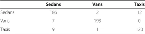
Sedans Taxis
Sedans 193 7
Taxis 1 129
Table 3 Confusion matrices using PCA + DFVS: sedans vs vans vs taxis
Sedans Vans Taxis
Sedans 189 1 10
Vans 8 190 2
As a result of intra-class variation in appearance and low resolution of images, the individual edge points are not sufficient to model spatial repeatability. Therefore, we group the similar descriptors that results in edge point groups that are spatially repeatable. The other benefit of using edge point groups is that it results in concise models compared to using edge points directly. In [4], Ma and Grimson used mean-shift clustering to create the edge point groups. Although mean shift is a good technique to find the dominant modes, it is computationally intensive (time complexity:O(Tn2), whereTis the number of iter-ations, andnis the number of features) and sensitive to parameters like the Gaussian kernel bandwidth. Thus, we use K-means clustering withK =10 (time complexity: O(KnT), whereKis the number of clusters,Tis the num-ber of iterations, andnis the number of features). Figure 4 shows a sample image, detected edge points after applying the Canny edge detector, and edge point groups after ap-plying K-means clustering.
After clustering the SIFT descriptors, we have edge points with their coordinates (pixel coordinates are nor-malized to (0.0, 1.0)) and respective SIFT descriptors. We denote the number of points in cluster (segment) i
as Ji, the 2D coordinates of the jth (j= 1,…Ji) point in
segmentiasPij→, and the SIFT vector of the point asSij→. A feature descriptorfk(k= 1,…N, whereNis the
num-ber of edge points in an image) is defined using the
triplet pij→
n o
; sij→
n o
; ci→
n o
n o
, where ci→ is the average of
allSij→ of segmenti. The feature descriptors obtained from an image are denoted by F= {fi}. During the training
phase, we extract all the feature descriptors of all the im-ages related to a particular class and group them accord-ing toci→.
3.5.2 Constellation model
A constellation model is a probabilistic model of a set of characteristic parts with a variable appearance and spatial configuration [10,28]. Ferguset al.modeled the object as a constellation of parts where shape configuration of the parts was modeled as a joint Gaussian of object parts’ coordinates, and the appearance of individual parts was modeled by independent Gaussians [10]. In [4], Ma and Grimson modified this constellation model to classify vehicles in two-class problem. We extend the approach
50 60 70 80 90 100
Accuracy
Number of eigenvectors
(a)
50 60 70 80 90 100
Accuracy
Number of eigenvectors
(b)
50 60 70 80 90 100 5 10 15 20 25 30 35 40
5 10 15 20 25 30 35 40
5 10 15 20 25 30 35 40
Accuracy
Number of eigenvectors
(c)
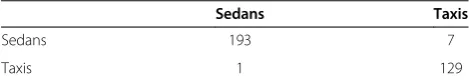
Figure 6Accuracy vs number of eigenvectors used (PCA + DIVS). (a)Cars vs vans.(b)Sedans vs taxis.(c)Sedans vs vans vs taxis.
Table 4 Confusion matrices using PCA + DIVS: cars vs vans
Cars Vans
Cars 199 1
Vans 2 198
Table 5 Confusion matrices using PCA + DIVS: sedans vs taxis
Sedans Taxis
Sedans 167 34
to multi-class classification and use a mixture of Gauss-ians (up to 6) to fit the model parameters.
Forcclassesω1,…ωc, a Bayesian decision is given by
C¼ arg max
c pðωcjFÞ ¼ arg maxc p Fð jωcÞpð Þωc ð15Þ
where Fcontains the features of an observed object. By assuming constant priors, a hypothesis is defined as matching of detected features to parts. Then, the likeli-hood can be expanded as
p Fð jωcÞ ¼ X
hϵHp Fð ;hjωcÞ
¼X
hϵHp F hð j ;ωcÞp hð jωcÞ;
ð16Þ
where H is the set of all possible hypotheses. In [4], it was observed that over-segmentation of edge points of an observed object may result in several almost identical features that effectively produce many-to-one hypothesis mapping. Ma and Grimson [4] used an approximation, where only the most probable hypothesis is used instead of summing over the entire hypothesis space for all the combinations. Therefore, Equation16becomes
p Fð jωcÞ≅p Fð ;hjωcÞ; ð17Þ
where h* is the hypothesis, in which every fi(fi ∈ F) is
mapped to the most similar part in a model. We assume that features of an object are independent of each other, and for each feature, assume that its edge point coordi-nates pij
→
n o
and corresponding SIFT vectors s→ij n o
are also independent. If we consider that there areNfeatures, then Equation16can be written as
p Fð jωcÞ≅ YN
i¼1p pij
→
n o jh;ωc
p s→ij n o
jh;ωc
ð18Þ
We consider two variations of this model: implicit shape model and explicit shape model as discussed in [4]. In the implicit shape model, we do not model the position of the features. Therefore, Equation 18 becomes
p Fð jωcÞ≅ YN
i¼1p sij
→
n o jh;ωc
ð19Þ
By assuming the independence of features, we can
calculatep sij→
n o jh;ωc
as
p s→ij n o
jh;ωc
¼ XKshð Þi m¼1 α
s hð Þi;m G s→ij
n o jμs
hð Þi;m;Σshð Þi;m
;
ð20Þ
whereh*(i) is the index of the part that matches feature
iof the observed object, Ks
hð Þi is the number of mixture
components, αs
hð Þi;m is the weight of the mth mixture
component, and μs
hð Þi;m andΣshð Þi;m are the mean vector
and covariance matrix of the mth Gaussian component, respectively. We use a mixture of Gaussians instead of a single Gaussian as used in [4]. It allows us to handle problems in clustering such as undersegmentation.
In case of the explicit shape model, we use Equation
18, wherep sij→
n o jh;ωc
is defined by Equation 20, and
p pij→
n o jh;ωc
is given by
p pij
→
n o jh;ωc
¼XKphð Þi m¼1α
p hð Þi;m G s→ij
n o jμp
hð Þi;m;Σ p hð Þi;m
;
ð21Þ
whereh*(i) is the index of the part that matches feature
iof the observed object, Kphð Þi is the number of mixture
components, αphð Þi;m is the weight of the mth mixture
component, and μphð Þi;m andΣphð Þi;m are the mean vector
and covariance matrix of the mth Gaussian component, respectively.
3.5.3 Learning and recognition
During the learning process, we have a choice of using all the features detected. However, it was observed by Ma and Grimson [4] that some features only appear in very few objects. Therefore, we can prune such features without losing the correctness of the model.
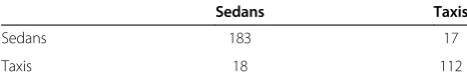
Table 6 Confusion matrices using PCA + DIVS: sedans vs vans vs taxis
Sedans Vans Taxis
Sedans 186 2 12
Vans 7 193 0
Taxis 9 1 120
Table 7 Confusion matrices using PCA + SVM: cars vs vans
Cars Vans
Cars 200 0
Vans 147 53
Table 8 Confusion matrices using PCA + SVM: sedans vs taxis
Sedans Taxis
Sedans 131 69
Taxis 78 122
Table 9 Confusion matrices using LDA: cars vs vans
Cars Vans
Cars 200 0
We use a similar learning and recognition procedure as outlined in [4]. We start by computing the features of each training sample in a class first. Then, sequential clustering is carried out on all features to give a feature pool. For sequential clustering, we denote a pool of features for class c as Fcq. To start, a training sample from classcwith all its featuresF= {fi} is randomly selected
and added to the feature pool. Then, another sample with all its featuresF′= {f′i} is added. For eachf′i,x2-distance is
calculated between the average SIFT feature vector ci.
Supposefminin the feature pool has the smallest distance tof′i. If this smallest distance is less than a threshold,f′iis
merged withfminin the feature pool by adding all its SIFT vectors and corresponding coordinates to fmin, and the mean SIFT vector of fmin is updated. Otherwise, f′i is
added toFc
qas a new feature. We repeat the same proced-ure for all training samples in classcto create the feature poolFcq. While creating feature pool, we also keep record of the percentage of sample images that contributed to feature fi which is denoted by ri. During the pruning
process, any featurefiwith ri less than some threshold is
considered to be invalid and not considered in the future model learning process.
For the model structures established in the previous sec-tion, the parameters to be learned are Kp
q;αpq;m;μpq;m;
n
Σp
q;m;Ksq;αsq;m;μsq;m;Σsq;mg, wherem= 1,…Kp,q= 1,…Q,
where Qis the number of parts in the feature pool. The parameters of Gaussian mixture models are estimated using a typical EM algorithm.
In the recognition phase, the features of an observed ob-ject are computed, and class conditional likelihoods are evaluated using Equation 18 for explicit shape model or Equation 19 for implicit shape model. The Bayesian deci-sion rule in Equation 16 gives the classification result.
3.6 A fusion of approaches
We presented five approaches that can be used in com-bination with each other and improve the classification
accuracy. The fusion of approaches becomes more import-ant when the number of classes increases. In Section 4, we present the results using all the approaches showing that certain approaches are better suited for a certain classifica-tion task, e.g., PCA + DIVS works well for the case ofcars vsvans, while PCA + DFVS works well for the case of se-dans vs taxis. As explained earlier, sedans and taxis are disjoint subsets ofcars. Therefore, we train two classifiers where the first classifier uses PCA + DIVS and classifies a test image intocars and vans. The test images that were classified as cars are further classified into sedans and taxis using the second classifier which employs PCA + DFVS. The fusion of different methods is thus possible and yields better results than just using a single approach.
4 Results
In this work, we have considered five different approaches. This section provides details about the experimental setup used during testing, the effect of different parameter choices on the results, and the comparison between the different approaches.
4.1 Experimental setup
In our dataset, we have three types of vehicles: cars, vans, andtaxis. Sedansandtaxisare the disjoint subsets of class cars. The dataset provided in [4] has 50 images of each class for training and 200 images of cars, vans, andsedanseach and 130 images oftaxis. For the case of carsvsvans, we use 50 images from each class for train-ing and 200 images of each class for testtrain-ing. For the case ofsedans vstaxis, we use 50 images from each class for training, while 200 images of sedans and 130 images of taxis are used for testing. We use the same experimental setup as that used in [6,7], so that a fair comparison is performed. In the case ofsedans vsvansvstaxis, we use 50 images of each class for training and 200 images of sedans, and 200 images of vans and 130 images of taxis for testing. Previously published results do not consider such as a three-class case.
Table 10 Confusion matrices using LDA: sedans vs taxis
Sedans Taxis
Sedans 194 6
Taxis 10 120
Table 11 Confusion matrices using LDA: sedans vs vans vs taxis
Sedans Vans Taxis
Sedans 174 6 20
Vans 17 180 3
Taxis 7 0 123
Table 12 Confusion matrices using implicit shape model: cars vs vans
Cars Vans
Cars 191 9
Vans 6 194
Table 13 Confusion matrices using implicit shape model: sedans vs taxis
Sedans Taxis
Sedans 183 17
4.2 Eigenvehicle approach (PCA + DFVS)
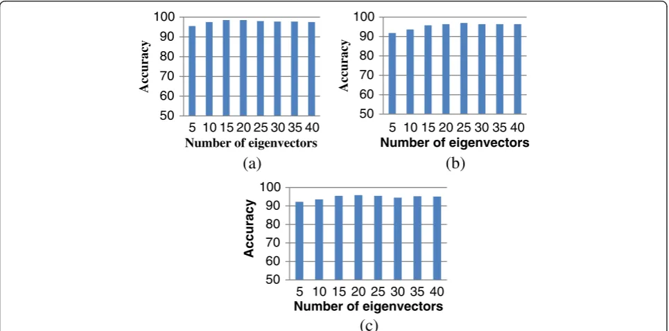
As 50 images of each class were used for training, the dimension of the principal component space is limited to 50. The first principal component (eigen) vector is the most expressive vector, the second one is the sec-ond most expressive vector, and so on. We choose the first k principal components and perform the experi-ment. Figure 5 shows the accuracy vs number of eigen-vectors used. We observed that changing the number of eigenvectors used does not change the accuracy greatly. For the case of sedans vs vans vs taxis, we achieved the accuracy of 95.85% when we used 20 eigenvectors. We got the accuracy of 98.5% in the case of carsvsvansby using 15 eigenvectors, while 97.57% in the case ofsedansvstaxisby using 22 eigenvectors. Tables 1, 2 and 3 give the confusion matrices for the experiments performed while using optimal number of eigenvectors.
4.3 PCA + DIVS
In this approach, we create a single combined principal component space for all the classes. During recognition, we have to make a similar choice as in the previous ap-proach to choose the number of eigenvectors that are used to calculate the Mahalanobis distance from the mean principal component vector of each class. We experimented with the choice of the number of eigen-vectors. Figure 6 shows the bar graphs of the accuracy vs number of eigenvectors.
For the case ofsedansvsvansvstaxis, we achieved an accuracy of 94.15% when we used 25 eigenvectors. Ac-curacy was 99.25% in the case of carsvsvans by using 40 eigenvectors, which is higher than any published results [6,7]. We achieved the accuracy of 89.69% in the case of sedans vs taxis by using 25 eigenvectors. Tables 4, 5 and 6 give the confusion matrices for the experiments performed while using optimal number of eigenvectors.
4.4 PCA + SVM
We used PCA + SVM to classifycarsvs vansandsedans vs taxis. We achieved an accuracy of 63.25% in the case ofcarsvsvansand 76.67% in the case ofsedansvstaxis. The accuracy achieved was low compared to other methods and therefore we did not perform the experi-ment on the more challenging case of sedans vsvans vstaxis. Tables 7 and 8 give the confusion matrices for the experiments performed.
4.5. LDA
LDA has shown to outperform PCA in the cases where there are many training samples [29]. In this algorithm, the number of nearest neighbors usedkis the free vari-able. We experimentally chose [k= 5]. We observed an accuracy of 96% in the case ofcars vs vansand 95.15% in the case of sedansvs taxis. In the difficult case of se-dansvsvansvstaxis, we achieved an accuracy of 90.00%. Tables 9, 10 and 11 give the confusion matrices for the ex-periments performed.
4.6 Constellation model
We consider two types of constellation models: implicit and explicit. In the implicit shape constellation model, we do not model the positions of the features. Tables 12, 13 and 14 give the confusion matrix for all the cases considered using the implicit shape model.
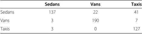
Using the implicit shape model, we achieved an ac-curacy of 96.25% in the case ofcarsvsvans, 89.39% in the case of sedansvs taxis, and 85.66% in the case of sedansvsvansvstaxis. In the explicit shape model, we model the normalized position of the features along with the features themselves. We achieved slightly bet-ter results forcarsvsvansand sedansvsvansvstaxis. However, the implicit shape model outperformed the explicit shape model in the case ofsedansvstaxis. We achieved a 97% accuracy in the case ofcarsvsvansand 89.09% in the case of sedansvstaxisusing the explicit shape model. In the difficult case when all three vehicle Table 14 Confusion matrices using implicit shape model:
sedans vs vans vs taxis
Sedans Vans Taxis
Sedans 137 22 41
Vans 3 190 7
Taxis 3 0 127
Table 15 Confusion matrices using explicit shape model: cars vs vans
Cars Vans
Cars 194 6
Vans 6 194
Table 16 Confusion matrices using explicit shape model: sedans vs taxis
Sedans Taxis
Sedans 183 17
Taxis 19 111
Table 17 Confusion matrices using explicit shape model: sedans vs vans vs taxis
Sedans Vans Taxis
Sedans 137 22 41
Vans 3 194 3
classes were considered, we achieved an accuracy of 86.04%. Tables 15, 16 and 17 give the confusion matrices for the experiments performed.
For both the implicit and explicit shape models, prior probabilities were considered to be the same. In the case of three class classification, we can observe that sedans are misclassified. We can alleviate this problem and im-prove the results by using higher prior probabilities for the sedan class.
4.7 A fusion of approaches
In this approach, we employ two classifiers: PCA + DIVS to classify between cars and vans, and PCA + DFVS to classify between sedans and taxis. For initial classifica-tion, we use the PCA + DIVS as explained in Section 3.2. To classify the images that are classified ascars, we use the PCA + DFVS as discussed in Section 3.1. We use this combined approach to classify vehicles in case ofsedans vs vansvs taxisand achieve an accuracy of 96.42%. The fusion approach works better than using any individual approach. Table 18 gives the confusion matrix for the experiment performed.
4.8 Comparison of approaches
In this paper, we used six different approaches to classify vehicles. The dataset that we used contains the images of vehicles taken from a surveillance video camera and segmented using a tracking algorithm [30]. The images were taken such that vehicles are captured in a more general oblique view instead of side or top view. We compare our approaches with the approaches presented in [4] and [8] that use the same dataset. We observe that our PCA + DFVS outperforms all other approaches in
the casesedansvstaxis, while our PCA + DIVS outper-forms the rest in the case ofcarsvsvans. In the case of sedansvsvansvstaxis, the proposed fusion of approaches (PCA + DIVS and PCA + DFVS) gives the best results.
The constellation model-based approach presented in this paper gives performance benefits by using K-means clustering over mean shift. It also has an advantage over all other approaches presented in this work that it has an ability to handle partial occlusions, owing to its reliance of local features rather than global features. Our constella-tion model-based approach gives comparable results to the constellation model-based approach presented in [4] for the cases ofcarsvsvansandsedansvstaxis.In this work, we extended the constellation model-based ap-proach to handle multi-class case. We can observe that the accuracy decreases while doing multi-class classifi-cation which can be attributed to increased number of common features as the number of classes increases.
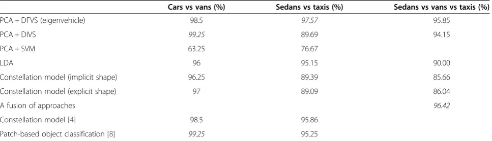
Table 19 provides the accuracy achieved using each approach, and the approaches that yielded the best results are italicized. The first seven rows of Table 19 provide the results obtained using techniques investigated in this paper. The last two rows of the Table 19 give the results obtained by the state-of-the-art techniques in vehicle classification when applied to the same dataset. They are copied from [4] and [8] respectively and use the same experimental setup as presented in this paper. However, these techniques do not extend to perform multi-class classification.
5 Conclusion
In this work, we investigated and compared five different approaches for vehicle classification. Using the PCA + DFVS (eigenvehicle) approach, we were able to achieve an accuracy of 97.57% in the challenging case of sedans vs taxiswhich is higher than any published results using this dataset. PCA + DIVS outperformed all other approaches investigated in this paper in the case ofcars vsvans. We also extended the constellation model approach [4] for classifying all three vehicle classes at the same time. LDA Table 18 Confusion matrix using a fusion of approaches
Sedans Vans Taxis
Sedans 189 3 8
Vans 4 194 2
Taxis 1 1 128
Table 19 Comparison of approaches
Cars vs vans (%) Sedans vs taxis (%) Sedans vs vans vs taxis (%)
PCA + DFVS (eigenvehicle) 98.5 97.57 95.85
PCA + DIVS 99.25 89.69 94.15
PCA + SVM 63.25 76.67
LDA 96 95.15 90.00
Constellation model (implicit shape) 96.25 89.39 85.66
Constellation model (explicit shape) 97 89.09 86.04
A fusion of approaches 96.42
Constellation model [4] 98.5 95.86
performed reliably but did not produce the best results in any of the cases we experimented on. PCA + SVM did not perform satisfactorily, but more experimentation with the choice of kernel and parameters might improve the results. Overall, PCA + DFVS approach achieves good results. However, the constellation model-based approach can be configured to work better in the presence of partial occlusion and minor rotations. We also presented an approach that combines two approaches and achieves improvements over using just one approach. We report accuracy of 96.42% in case of sedans vs vans vs taxis using a fusion of approaches. We can use the SIFT-PCA features to train the constellation models. Also, features other than SIFT, such as LoG affine regions can be used for modeling. The performance of the constellation model deteriorates as we extend it to multiple classes. A boosting algorithm can be used to choose the appropriate features for training.
In this paper, we used the images extracted from sur-veillance video captured using a fixed-angle camera. In the real traffic surveillance videos, vehicles can have different orientations and different view angles and sizes. The problem of orientation can be solved using camera self-calibration and the result of a tracking algo-rithm. Appearance-based algorithms have limited ability to model different view angles. A 3D model-based approach with strong thresholds (low false positives) can be used to train an appearance-based approach for better accuracy.
Competing interests
The authors declare that they have no competing interests.
Acknowledgements
This work has been supported by the Office of Naval Research, under grant number N00014-09-1-1121.
Received: 30 July 2012 Accepted: 23 April 2014 Published: 10 June 2014
References
1. USDOT, USDOT intelligent transportation systems research. (2011). http://www.fhwa.dot.gov/research/. Accessed 22 Jan 2013 2. D Ang, Y Shen, P Duraisamy,Video analytics for multi-camera traffic
surveillance(Paper presented at the second international workshop on computational transportation science, Seattle, WA, USA, 2009), pp. 25–30 3. A Ambardekar, M Nicolescu, G Bebis,Efficient vehicle tracking and
classification for an automated traffic surveillance system(Paper presented at the international conference on signal and image processing, Kailua-Kona, HI, USA, 2008), pp. 1–6
4. X Ma, W Grimson,Edge-based rich representation for vehicle classification
(Paper presented at the international conference on computer vision, New York, NY, USA, 2006), pp. 1185–1192
5. M Turk, A Pentland, Eigenfaces for recognition. J. Cogn. Neurosci. 3(1), 71–86 (1991)
6. N Buch, J Orwell, S Velastin,Three-dimensional extended histograms of oriented gradients (3-DHOG) for classification of road users in urban scenes
(Paper presented at the British machine vision conference, London, UK, 2009)
7. J Canny, Computational approach to edge detection. IEEE Trans. Pattern Anal. Machine Intell.PAMI-8, 679–698 (1986)
8. R Wijnhoven, P de With,Experiments with patch-based object classification
(Paper presented at the IEEE conference on advanced video and signal based surveillance, London, U.K, 2007), pp. 105–110
9. D Swets, J Weng, Using discriminant eigenfeatures for image retrieval. IEEE Trans. Pattern Anal. Machine Intell.18(8), 831–836 (1996)
10. R Fergus, P Perona, A Zisserman,Object class recognition by unsupervised scale-invariant learning(Paper presented at the IEEE conference on computer vision and pattern recognition, Madison, WI, USA, 2003), pp. 264–271
11. L Fei-Fei, R Fergus, P Perona,Learning generative visual models from few training examples: an incremental Bayesian approach tested on 101 object categories(Paper presented at the IEEE conference on computer vision and pattern recognition, Washington D.C., USA, 2004)
12. H Kollnig, H Nagel, 3D pose estimation by directly matching polyhedral models to gray value gradients. Int. J Comput. Vision23(3), 283–302 (1997) 13. J Lou, T Tan, W Hu, H Yang, S Maybank, 3-D model-based vehicle tracking.
IEEE Trans. Image Processing14(10), 1561–1569 (2005)
14. R Wijnhoven, P de With,3D wire-frame object modeling experiments for video surveillance(Paper presented at the international symposium on information theory, Seattle, WA, USA, 2006), pp. 101–108
15. S Gupte, O Masoud, RFK Martin, N Papanikolopoulos, Detection and classification of vehicles. IEEE Trans. Intell. Transport. Syst.3(1), 37–47 (2002) 16. R Avely, Y Wang, G Rutherford,Length-based vehicle classification using
images from uncalibrated video cameras(Paper presented at the intelligent transportation systems conference, Washington, WA, USA, 2004)
17. Z Chunrui, M Siyal,A new segmentation technique for classification of moving vehicles(Paper presented at the vehicular technology conference, Boston, MA, USA, 2000), pp. 323–326
18. C Zhang, X Chen, W Chen,A PCA-based vehicle classification framework
(Paper presented at the international conference on data engineering workshops, Atlanta, GA, USA, 2006), pp. 17–17
19. D Lowe, Distinctive image features from scale-invariant keypoints. Int. J. Comput. Vis.60(2), 91–110 (2004)
20. K Mikolajczyk, C Schmid,A performance evaluation of local descriptors(Paper presented at the computer vision and pattern recognition, Madison, WI, USA, 2003), pp. 257–263
21. M Koch, K Malone,A sequential vehicle classifier for infrared video using multinomial pattern matching(Paper presented at the conference on computer vision and pattern recognition workshop, New York, NY, USA, 2006), pp. 127–133
22. K Simonson,Multinomial Pattern Matching: A Robust Algorithm for Target Identification(Automatic Target Recognizer Working Group, Huntsville, 1997) 23. C Huang, W Liao,A vision-based vehicle identification system(Paper
presented at the international conference on pattern recognition, Cambridge, UK, 2004), pp. 364–367
24. P Ji, L Jin, X Li,Vision-based vehicle type classification using partial Gabor filter bank(Paper presented at the international conference on automation and logistics, Jinan, China, 2007), pp. 1037–1040
25. B Schölkopf, J Platt, J Shawe-Taylor, A Smola, R Williamson, Estimating the support of a high-dimensional distribution. Neural Comput.13(7), 1443– 1471 (2001)
26. R Fisher, The statistical utilization of multiple measurements. Annals of Eugenics8(4), 376–386 (1938)
27. K Mikolajczyk, T Tuytelaars, C Schmid, A Zisserman, J Matas, F Schaffalitzky, T Kadir, L Van Gool, A comparison of affine region detectors. Int. J. Comput. Vis.65(1–2), 43–72 (2005)
28. M Burl, M Weber, P Perona,A probabilistic approach to object recognition using local photometry and global geometry(Paper presented at the European conference on computer vision, Freiburg, Germany, 1998), pp. 628–641
29. AM Martinez, AC Kak, PCA vs LDA. IEEE Trans. Pattern Anal. Machine Intell. 23(2), 228–233 (2001)
30. J Migdal, W Grimson,Background subtraction using Markov thresholds
(Paper presented at the IEEE workshop on motion and video computing, Breckenridge, CO, USA, 2005), pp. 58–65
doi:10.1186/1687-5281-2014-29
Cite this article as:Ambardekaret al.:Vehicle classification framework: a comparative study.EURASIP Journal on Image and Video Processing