statistical physics approach
Alamino, R.C., Saad D.Aston University, Neural Computing Research Group, Birmingham B4 7ET, UK
Using methods of statistical physics, we study the average number and kernel size of general sparse random matrices overGF(q), with a given connectivity profile, in the thermodynamical limit of large matrices. We introduce a mapping ofGF(q) matrices onto spin systems using the representation of the cyclic group of order q as the q-th complex roots of unity. This representation facilitates the derivation of the average kernel size of random matrices using the replica approach, under the replica symmetric ansatz, resulting in saddle point equations for general connectivity distributions. Numerical solutions are then obtained for particular cases by population dynamics. Similar tech-niques also allow us to obtain an expression for the exact and average number of random matrices for any general connectivity profile. We present numerical results for particular distributions.
PACS numbers: 02.10.Yn, 02.70.-c,05.10.-a
Keywords: random matrices, Galois fields, statistical mechanics, replica theory
I. INTRODUCTION
Random matrices over GF(q) are highly important in a number of application areas ranging from biology to computer science and telecommunication. One of the areas where they play a particularly important role is coding theory [1]. In particular, linear codes are defined by the kernel of a parity-check matrix, where each kernel vector is termed a codeword and is associated with an original uncoded message vector by a linear operation defined by a generator matrix. Well known examples include the Hadamard codes, where properties of the kernel and rank play an important role [2], and low-density parity-check codes (LDPC) which provide the best performance to date in many noise regimes. Although the most studied and applied case of LDPC codes is of binary codes overGF(2) there is a significant body of work, of both practical and theoretical nature [3], on codes over more general finite fields showing an improvement in performance with respect to the binary version. In particular, statistical physics based analysis of LDPC codes overGF(q) has been reported in [4].
Low-density parity-check codes are based on random sparse matrices, where the fraction of non-zero elements goes to zero as the size of the matrix increases. In most studies of LDPC codes, it is assumed that a parity-check matrix withM rows (parity-checks) andN columns defines a code of rateR= 1−M/N,exactly, which is equivalent to the assertion that the number of vectors in the kernel (and therefore the number of codewords) is exactlyqN R.
In addition to being an interesting applied problem, the properties of these matrices are also of great interest from the pure mathematical point of view and a number of papers has already tried to answer related questions in different instances with a mathematical rigorous approach [5–7].
Random matrices are a well studied topic in the physics community where they are important in a range of applications from classical physics to quantum chaos. Recently there has been a lot of activity in the area boosted by the application of techniques originated in the statistical mechanics of disordered systems [8–13]. These techniques have been used to analyse ensemble properties and the replica method has proved to be a valuable tool in several of these approaches. Differently from this paper, however, most of other works concentrate in the spectral properties of the matrices. Also, in most cases, the studied matrices are real, while the restriction to GF(q) matrices considered here makes the solution of the problem more involved.
In this contribution, we address two key properties of sparse random matrices over GF(q), namely the average dimension of their kernel and the number of matrices for a given connectivity profile, in the case of large matrices. When the matrices are large, keeping N → ∞ with M/N constant, the problem can be mapped into a system of interacting “spins” and the powerful machinery developed for the study of disordered spin lattices in condensed matter physics can then be used, under some assumptions, to obtain the required properties.
II. KEY CONCEPTS
A. GF(q)-Matrices
A Galois fieldGF(q) is a finite field withqelements, i.e., a set ofqelements{0, ..., q−1}, which we symbolize by integers for convenience, which is a commutative group under addition⊕:GF(q)→GF(q), defined as integer addition
mod q, and with a monoid structure with respect to a commutative multiplication operation ⊗:GF(q)→ GF(q). The field also includes the zero element ’0’, mapping every other element to itself, and the identity ’1’; an additional requirement is that the multiplication and addition have the algebraic distributive property. This last requirement restricts the number of elements to beq=pn, wherepis a prime number andnan integer.
Entries in matrices overGF(q) take values of numbers in the field GF(q), where the usual additions and multi-plications involved in their algebra are defined by the corresponding operations over the Galois field. The kernel, or
null space, of anM×N matrixA is defined as the set of vectorsv∈GF(q)N such thatAv= 0, with all operations in the fieldGF(q). The kernel is a linear vector space and therefore will haveqd(A) vectors, whered(A) is the kernel dimension. The rankr(A) of the matrix is obtained by the rank-nullity theorem asr(A) =N−d(A).
B. Disordered Systems
An interacting spin problem has two main elements: an interaction defined between a number of spin units, collectively represented by the vector σ = (σ1, ..., σN), in a lattice and a local field which acts in each variable σi
separately. Disordered spin systems are systems where one or both of these elements (interaction and field) is a random variable. Usually, we are interested in the properties of very large systems, where the number N of spins becomes infinite, the so-called thermodynamic limit.
The main properties of the system in the thermodynamic limit can be derived from a key quantity, the free-energy f, which in probabilistic terms corresponds to the cummulant generating function. For disordered systems, in the cases where the free-energy is self-averaging with respect to the disorder, we can calculate this quantity as
f =− lim
N→∞
1
βNhlnZi, (1)
whereh·i indicates the disorder average,Z =P
σe
−βH(σ) is the partition function andH(σ) is the Hamiltonian of the system. Although the self-averaging property should be rigorously investigated for each system, we will assume it holds here.
In order to obtain the free-energy, a powerful technique is to make use of the replica method, based on the identity
∂ ∂nlnhZ
ni
n=0
=hlnZi. (2)
Average quantities can then be calculated for integernand then analytically continued to zero. The replica theory is commonly used in the area of disordered systems and is known to provide exact results in many regimes, which include both physical and non-physical systems [14, 15].
Many problems in computing and communication theory can be mapped to spin systems. For instance, error-correcting codes, in particular LDPC codes [16] and hard computational problems such as K-SAT [17] and graph-coloring [18, 19], can be mapped to diluted spin systems with random p-spin interactions and local fields. In the coding example, interactions are defined by the parity-check constraints, while the local fields are induced by the codeword and received message. In the statistical physics treatment, for mathematical convenience, the message bits {0,1} and ’⊕’ operation are mapped onto spin values {+1,−1} and multiplication using the mapping x→ (−1)x.
Variables over a general finite fieldGF(q),q6= 2 are typically first mapped onto a binary string and then, using the spin values representation, transformed into a spin system [4].
III. MAPPINGGF(q)MATRICES INTO SPIN SYSTEMS
The transformation
σ(v) = (−1)v, (3)
Under the operation⊕,GF(q) is homeomorphic to the cyclic group of order qand therefore has a representation as the complexq-th roots of unity with the group homeomorphismσ:GF(q)→Cgiven by
σ(v) = exp
2πi q v
, (4)
such that for everyv1, v2∈GF(q)
σ(v1⊕v2) = exp 2πi
q (v1⊕v2)
= exp
2πi
q (v1+v2)
= exp
2πi q v1
exp
2πi
q v2
=σ(v1)σ(v2).
(5)
This mapping has a clear geometric interpretation: 2πv/q is an angle in the unit circle, such that each element of the Galois field is being mapped onto a spin variable “pointing” in one ofq possible angles. Using this mapping allows one to write the null-space constraint for a general vectorv= v1, ..., vN
∈GF(q)N as
δ(Av,0) =
M
Y
i=1 δ
N
M
j=1
Aij⊗vj
,0
, (6)
with
δ
N
M
j=1
Aij⊗vj,0
= 1 ∆(q)
q−1 Y
m=1
1−exp
−2πi
q m
N
Y
j=1 exp
2πi
q Aij⊗v
j
, (7)
and
∆(q) =
q−1 Y
m=1
1−exp
−2πi q m
. (8)
Using the properties of the complex roots of unity, the above quantity ∆(q) can be shown (see appendix A) to be real and equal to the orderqof the field.
Based on this representation, we can now define the “magnetization” of the original system in analogy with the spin system as
m= 1 N
N
X
j=1
σj, (9)
and the overlap between two configurationsσ andσ0 as
ρ= 1 N
N
X
j=1
σjσ0j, (10)
where we are now working with the spin variables already mapped to the the complex field C and therefore the
operations of multiplication and addition correspond to the usual ones inC.
It turns out that this kind of representation allows a factorization of the terms simplifying the equations and making the replica calculations simpler, as we will see in the following.
IV. AVERAGE PROPERTIES OF THE KERNEL
The dimension of the kernel of anM×N matrixAoverGF(q) can be written asd(A) = logqΩ where
Ω =X
v
is the number of vectors in the kernel, δ is the Kroenecker delta and v ∈ GF(q)N. Direct calculation of Ω from equation (11) by straightforwardly substituting the Kroenecker delta by its integral representation trivially reproduces the rank-nullity theorem. This calculation is not presented here.
The quantity we are interested in here is the average kernel dimension, more specifically, its density in the limit of large matrices, defined asT swhere
s≡ 1 T Nlim→∞
hd(A)iA
N = limN→∞ 1
Nhln ΩiA, (12)
where 1/T = lnqandM/N ≡λ, with λa finite positive constant. Using the replica identity (2), we can write s= lim
N→∞
∂ ∂nlnhΩ
ni A
n=0
. (13)
The randomly chosen sparse matricesAhave exactlyKi non-zero elements in thei-th row with probabilityP(K),
K ≡ (K1, ..., KM), and Cj elements in the j-th column with probability P(C), C ≡ (C1, ..., CN), obeying the constraint Λ≡P
iKi =
P
jCj, where Λ is the total number of non-zero elements of the matrix. The elements of A
are sampled from the finite fieldGF(q) with independent equal probabilitiesP(Aij).
Let us define, for brevity of notation,Zn ≡ hΩniA. Although the calculations, presented in appendix B, are similar
to related calculations in [20, 21], we will use a different approach which is conceptually clearer and has the advantage of allowing later generalizations. In this approach, we sum directly over all entries of the matrix instead of defining a connectivity tensor as used elsewhere [20, 21],
Zn=
* 1 N
X
{Aij}
Y
i,j
P(Aij)
M Y i=1 δ N X j=1
χ(Aij), Ki
N Y j=1 δ M X i=1
χ(Aij), Cj
! × n Y a=1 " X va
δ(Ava,0)
#+
K,C,Λ ,
(14)
where the average is over the probability distributionP(K,C,Λ) with χ(Aij) = 0 if Aij = 0 and 1 otherwise, and the normalizationN gives the number of matrices which obey the constraints averaged over the distributions of the entries. In this way, any type of constraint on the matrix can be readily included in the calculation, which could be rather cumbersome in other approaches, based on the introduction of a connectivity tensor as the corresponding constraints have to be written in terms of the tensor elements, which can be extremely complicated.
We refer the reader to appendix B for details of the calculations. Using the replica symmetric ansatz, which is shown to be exact for this problem (see appendix D) we arrive at the following self-consistent saddle point equations
ˆ
π(ˆx) = 1 α(α) M X i=1 * αΛ
Λ!Kiδ xˆ−
Ki−1 Y
l=1 xl
!+
x,K,C,Λ
, (15)
π(x) = 1 α(α) N X j=1 * αΛ
Λ!Cjδ x−
QCj−1
l=1 [1+(q−1)ˆxl]−QC
j−1
l=1 (1−xˆl)
QCj−1
l=1 [1+(q−1)ˆxl]+(q−1)QC
j−1
l=1 (1−xˆl)
!+
ˆ x,K,C,Λ
, (16)
0 = αΛ
Λ!
1−Λ α
K,C,Λ
, (17) with (α) = αΛ Λ!
K,C,Λ
, (18)
and to the corresponding expression fors s=−λlnq− α
Nhln [1 + (q−1)xˆx]ix,xˆ
+ 1 N (α) X i * αΛ Λ! * ln "
1 + (q−1)
Ki Y l=1 xl #+ x +
K,C,Λ
+ 1 N (α) X j * αΛ Λ! * ln Cj Y l=1
[1 + (q−1)ˆxl] + (q−1) Cj Y
l=1
(1−xˆl)
+ ˆ x +
K,C,Λ
.
The probability distributions π(x) and ˆπ(ˆx) in equations (15) and (16) are of the auxiliary effective field x and its conjugate ˆx, respectively. They represent a generating function for the order parameters defined as site averages of a given number of system replicas. They can also be interpreted as message probability distributions within the microscopic message passing framework, also known as belief propagation[22]; a more detailed explanation is provided in [23, 24]. Their exact definition is given in equations (B17) and (B18) of appendix B.
It must be noted that the above equations are only meaningful if Λ∝N. A striking property of the above equations is that they arecompletely independent of the specific distribution of the individual elements of the matrix, depending only on the distribution ofKandC (and, obviously, of Λ).
There exists two straightforward analytical solutions of the above equations, namely, the paramagnetic one given by
ˆ
π(ˆx) =δ(ˆx), π(x) =δ(x), (20) and the ferromagnetic solution
ˆ
π(ˆx) =δ(ˆx−1), π(x) =δ(x−1). (21)
When substituted in the above equations, the paramagnetic solution gives the average kernel density as T s = 1−λ = 1−M/N independently of the orderq of the finite field used. In the case of LDPC codes defined by such matrices, this corresponds to random parity-check matrices that defines a code of rateR= 1−λ. The average rank density in this case is λ. The ferromagnetic solution gives T s= 0 and the matrix is full rank; which incidentally means that such matrices cannot be used to define a parity-check code due to the lack of redundancy.
These quantities can be associated to analogous quantities in the statistical mechanics framework. We start by associating the average rank density with the free-energyf and writing
f ≡ hr(A)iA
N = 1−T s, (22)
which allows one to associate s with the entropy and the internal energy density being constrained to be u = 1. Defining β= 1/T, equation (22) becomes
βf= 1− 1 N
* lnX
v
δ(Av,0)
+
A
= 1 N
*
Nlneβ−lnX
v
δ(Av,0)
+
A
=−1 N
* lnX
v
δ(Av,0)e−βN
+
A
=−1 N
* lnX
v
e−βH(v)
+
A
,
(23)
where the Hamiltonian of the corresponding statistical mechanical system is formally
H(v)≡N−lnδ(Av,0). (24)
We solved the saddle point equations by means of population dynamics for three different cases, in all of which we keepK fixed
1. Regular matrices -C andK fixed;
2. FixedK andCdrawn from a multinomial uniform probability
P(C) = (M K)!
Q
jCj!
1
NM K; (25)
0.0 0.5 1.0
λ
0.0 0.5 1.0
Kernel Dimension Rank
0.0 0.5 1.0
λ
0.0 0.5 1.0
Kernel Dimension Rank
0.0 0.5 1.0
λ
0.0 0.5 1.0
Kernel Dimension Rank
0.0 0.5 1.0
0.0 1.0
Kernel Dimension Rank
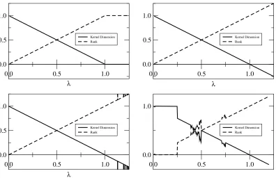
FIG. 1: Average kernel dimension density (continuous lines) and average rank density (dashed lines) calculated as solutions to the replica symmetric saddle point equations. The top left plot shows the thermodynamically favored solution (paramagnetic for 0≤λ≤1 and ferromagnetic forλ >1). The top right shows the regular case (i) for fixedKandC. Cases (ii) and (iii) are presented at the bottom left and right, respectively. Note that numerical instabilities occur for specificλvalues.
Population dynamics [25] is an iterative method to obtain the probability distributions of the auxiliary fields. Firstly, a large population of fieldsxand ˆxis generated and each individual is initialised to a random value in the interval [−1,+1]. Then, the whole population is sampled in a random order and updated according to the relations defined by the saddle-point equations. This process is repeated a large number of times and averaged over all realisations. The number of iterations in the algorithm is fixed due to the fact that close to the critical points it exhibits a critical slowing down and convergence of the population is extremely slow.
Results for the various cases are presented in Fig. 1. The top left plot shows the theoretical thermodynamically dominant solutions (paramagnetic in the range 0≤λ≤1 and ferromagnetic forλ >1) having the lower free energy. The top right plot shows the results for the regular case (i). Solutions were obtained numerically by iterating equations (15) and (16) for the case ofq= 4 andK = 200;C was varied from 2 to 250. Repeating the calculations for different values ofqandKhave produced similar results. We see that the stable solution is always paramagnetic, but becomes unphysical atλ= 1 once the entropy, and consequently the dimension of the kernel, becomes negative. In the case of parity-check codes, this result means that the typical parity-check matrix defines a code of rate exactly (N−M)/N. This is assumed for any parity-check matrix in most calculations in the literature and is confirmed by our results to be true on average; however, it is important to point out that the result is true in the limit of large matrices and is likely to have finite size corrections which may affect practical applications.
Cases (ii) and (iii) are presented, respectively, at the bottom left and right of Fig. 1. Although these cases do not rigorously obey the constraint that eachCj must be at mostM, for large matrices and small values of K (which is
what happens in practice)Cj is unlikely to exceed this value. However, instabilities can and indeed occur for specific
λvalues, presumably due to instances whereCj takes higher values.
The bottom left plot shows results for the case (ii), withq= 3,K= 4,N = 1000 and 1≤M ≤1250. Also in this case, the stable dominant solution is paramagnetic. Numerical instabilities, which disappear slowly with the increase in the number of fields and steps in the population dynamics, emerge in the unphysical region and are shown in the figure.
The behavior for case (iii) is a little more complex due to the nature of the distribution chosen. Using the average valueλK for the variablesCj implies that, asλvaries, their average value also changes. The plot shown was obtained
two points, where numerical instabilities emerge, are related to the percolation transition. Further calculations with differentKvalues indicate that these points appear around the extremes of the interval 2/K ≤λ≤3/K. Inside this interval, the average value of theCj’s equal to 2 (once we take it to be an integer). This value marks the percolation
transition for binary matrices; the numerical instabilities in this case are associated with a critical slowing down of the algorithm close to the transition point as the algorithm stops after a pre-determined number of iterations. Apart from these differences, the resulting curve seems to coincide with those obtained for the previous cases.
The solution of kernel size problem is mathematically equivalent to the solution of LDPC in channels with infinite noise. As the solution in the latter is paramagnetic, we are led to speculate that it is the dominant solution also here up to the point where the quantitys, analogous to the entropy, becomes negative. From this point and on the solution becomes ferromagnetic. The numerical results seem to support this conjecture, although more careful calculations, varying all the parameters involved must be carried out to confirm this hypothesis more generally.
V. NUMBER OF MATRICES
The number ofGF(q) matrices given a connectivity profile is of significant interest within the discrete mathematics community. Exact results have been obtained for the case offinitebinary matrices [26] in the form of a formula that facilitates the calculation of their precise number. In this paper we will analyze the case of largeGF(q) matrices and provide an expression for both their exact and average number. Given the precise number of non-zero elements per rowK= (K1, ..., KM) and per columnC= (C1, ..., CN), one can write the number of matrices as
NA=
X
{Aij}
M
Y
i=1 δ
N
X
j=1
χ(Aij), Ki
N
Y
j=1 δ
M
X
i=1
χ(Aij), Cj
!
. (26)
Note that we are using the summation directly over the entries of the matrix instead of the introduction of a connectivity tensor. In this way, the calculations are similar to the ones for obtaining the kernel dimension with the details given in C. The final result is
NA= (q−1)Λ
Λ! Q
iKi!QjCj!
. (27)
Note that the component on the right represents the number of binary matrices with the given non-zero elements profile. The factor (q−1)Λis the multiplicity of the non-zero entries which can have any non-zero value in the Galois field.
If we consider a distributionP(K,C,Λ), we can look at theaveragenumber of matrices
¯ NA=
*
(q−1)ΛQ Λ!
iKi!QjCj!
+
K,C,Λ
. (28)
Note that we can write the joint probability distribution as
P(K,C,Λ) =P(K|Λ,C)P(Λ|C)P(C), (29)
and thatP(Λ|C) =δΛ,P
jCj
. Therefore, we have obtained for the average number of matrices
¯ NA=
X
K
X
C
P(K|C)P(C)(q−1)PjCj
P
jCj
!
Q
iKi!QjCj!
, (30)
where the distributionP(K|C) includes the constraintδP
iKi,PjCj
.
A simple calculation shows that for the regular case, where allCj’s andKi’s are fixed (toC andK, respectively),
andq= 2, the number of matrices scales asNCN. Therefore, a more appropriate quantity to calculate instead of the
average number of matrices would be the quenched entropy
Ξ≡
1 N lnNA
= 1
N X
K
X
C
P(K|C)P(C) ln
(q−1)
P
jCj
P
jCj
!
Q
iKi!
Q
jCj!
TABLE I: Asymptotic values of Ξ∗for largeλ
¯
C As. Value 5 29.66 10 60.73 20 123.20
which scales as lnN.
We analyze the behavior of this quantity for three different cases. We choose each Cj to be i.i.d. and K to be
chosen from a multinomial distribution
P(K) =(
P
iKi)!
Q
iKi!
1 NP
iKiδ
X
i
Ki,
X
j
Cj
, (32)
for each realization ofC. The three probability distributions for the variablesCj to be analyzed are 1. uniform in the interval [0,2 ¯C]
P(Cj) = 1/(2 ¯C+ 1); (33)
2. binomial in the interval [0, M]
P(Cj) =
M Cj
C¯ M
Cj 1− C¯
M M−Cj
; (34)
3. Zipf distribution forCj = 1, ..., M
P(Cj) =
C−s j
PK
n=1n−s
, (35)
where ¯C is the mean of the distributions. The motivation for choosing these connectivity profiles is that they appear to be the most commonly analyzed and feature (especially the latter) in recent analysis and modelling of networks.
Results for the binomial (dashed line) and uniform (dotted line) distributions with means ¯C= 5.0,10.0,20.0,q= 2 andN = 300 are plotted in Fig. 2, together with the value of Ξ with constantCj = ¯C andKj= ¯C/λvalues for alli
andj. This function is explicitly given by
Ξ∗= ¯Cln(q−1)−ln ¯C! + 1
Nln (N C)!−λln ¯C/λ
!, (36)
and we can obtain its asymptotic behavior for small and largeλas
λ1⇒Ξ∗= ¯Cln(q−1)−ln ¯C! + ¯ClnλN, (37) λ1⇒Ξ∗= ¯Cln(q−1)−ln ¯C! + ¯Cln ¯CN+ (γ−1) ¯C, (38) whereγ≈0.577216 is the Euler-Mascheroni constant. Asymptotic limits for largeλare given in table I.
For largeλvalues the result for constantCandKupper-bounds the other two distributions. Additional calculations seem to indicate that it is always the case for any distribution, although a proof for this conjecture is still sought. This implies that if we keep the number of columns constant and increase the ratio λby adding rows, whenever the number of rows is much larger than the number of columns, the average number of matrices becomes independent of both the ratio and number of rows. The plots also suggest that the average number of matrices in these cases are basically defined by the average value of theCdistributions.
For small values of λ, the uniform distribution continues to be upper-bounded by the constant distribution. The binomial distribution, however, is higher for a small interval around zero. This behavior is shown in the inset where lowerC values give rise to higher Ξ asλbecomes smaller.
0.0 0.5 1.0 1.5 2.0
λ -40
-20 0 20 40 60 80
Ξ 5.0
10.0 20.0 Constant C and K
Binomial Distribution Uniform Distribution
0 0.07
0 20
FIG. 2: Values of the quenched entropy Ξ versusλ for the different distributions and variousC values (C= 5,10,20), with multinomial K: constant (continuous line), binomial (dashed line) and uniform (dotted line). The inset shows in detail the small λregime, where just the binomial and constant distributions are represented. The higher lines on the right correspond to the higherCvalues.
0.0 0.5 1.0 1.5 2.0
λ 0
100 200 300 400 500
Ξ
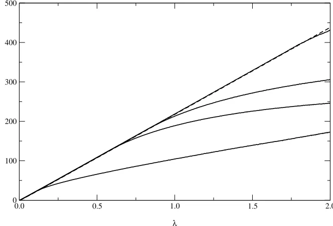
FIG. 3: Values of Ξ versus λ for the uniform distribution (dashed line) and the Zipf distribution (continuous lines) for
s= 1,3,4,10, respectively, from bottom to top.
VI. CONCLUSIONS
number of matrices under various connectivity profiles.
Using the replica approach and these new introduced techniques, we calculated the average dimension of the kernel for a general distribution of non-zero entries and solved the resulting equations numerically, finding that the average kernel density is 1−M/N in all cases studied. We conjecture that this result is always valid. Based on the analogy with thermodynamical quantities corresponding to free energy, internal energy and Hamiltonian, we showed that the replica symmetric ansatz in this case must be exact. With the same techniques, we were also able to find the total number of large matrices for fixedK andC and their average number, which was then computed for different distributions of theoretical and practical relevance.
The results presented have practical relevance in a number of areas, including coding network modelling and some biological models. With respect to LDPC codes, the average kernels density result implies that randomly generated LDPC codes typically define codes of rate exactly 1−M/N, an assumption which is generally made but lacks rigorous derivations. Also, as the parity-parity check matrix can represent the connectivities in graphs (see [27]), the results obtained for the average number of matrices provide a principled approach to determine the average number of possible graphs with a given connectivity distributions of a more general nature than the connectivity profiles examined in this paper.
Acknowledgements
We would like to thank the invaluable comments and suggestions of the anonymous referees. Support from EPSRC grant EP/E049516/1 is gratefully acknowledged. R.C.A. would also like to thank Dr. Juan P. Neirotti for useful discussions.
APPENDIX A: PROOF OF∆(q) =q
In this appendix we prove the statement made in section IV that ∆(q) =q where [29]
∆(q) =
q−1 Y
m=1
1−exp
−2πi q m
. (A1)
From the above equation, we have
∆(q) =
q−1 Y
m=1 exp
−πi
q m
exp
πi q m
−exp
−πi
q m
= (2i)q−1exp −πi q
q−1 X
m=1 m
!q−1 Y
m=1 sin
mπ
q
.
(A2)
The identity
exp −πi q
q−1 X
m=1 m
!
=i1−q, (A3)
implies the equation
∆(q) = 2q−1
q−1 Y
m=1 sin
mπ
q
. (A4)
Using the known identity [28]
sin(qx) = 2q−1
q−1 Y
m=0 sin
x+mπ q
, (A5)
divided by sinxand takingx→0, one obtains
q−1 Y
m=1 sin
mπ
q
= q
2q−1, (A6)
APPENDIX B: REPLICA SYMMETRIC SADDLE POINT EQUATIONS
Using integral representations for the first two sets of Kroenecker delta functions, we can write the averaged replicated kernel size defined in equation (14) as
Zn=
* 1 N
X
{va} I
DW DZ X {Aij}
Y
i,j
P(Aij)(WiZj)χ(Aij)
× M Y i=1 Y a δ N M j=1
Aij⊗vja
,0
+
K,C,Λ ,
(B1)
where⊗and⊕indicate multiplication and summation onGF(q), respectively, and
DW DZ= "M
Y
i=1 dWi
WKi+1
i # N Y j=1 dZj
ZCj+1
j
. (B2)
Using the representation of the parity-check constraint given in equation (6), the product over replica indices of the delta function can be written as
Y a δ N M j=1
Aij⊗vaj
,0 = Y a 1 q
q−1 Y
m=1
1−exp
−2πi q m N Y j=1 exp 2πi
q Aij⊗v
j a = 1 qn Y a " 1 +
q−1 X
s=1
Fi(s, a)G(s)
# = 1 qn n X r=0 X
ha1···ari X
s1,...,sr
G(s1)· · ·G(sr)Fi(s1, a1)· · ·Fi(sr, ar),
(B3)
with
G(s)≡ X hm1···msi
(−1)sexp
−2πi
q m1
· · ·exp
−2πi q ms
, (B4)
and
Fi(s, a)≡exp
2πi
q Ai1⊗v 1
a
· · ·exp 2πi
q AiN⊗v
N a = N Y j=1
γj(s, a, Aij),
(B5)
where we defined, for simplicity,
γj(s, a, Aij)≡exp
2πi
q s Aij⊗v
j a
. (B6)
We can now write the partition function as
Zn=
* 1 N
X
{va} I DZ M Y i=1 1 qn n X r=0 X
ha1···ari X
s1,...,sr
G(s1)· · ·G(sr)
I dW
i
2πi 1 WKi+1
i
Γi
+
K,C,Λ
where
Γi =
X
Ai1,...,AiN
Y
j
P(Aij)(WiZj)χ(Aij)
Y
j
γj(s1, a1, Aij)· · ·γj(sr, ar, Aij)
=Y
j
X
Aij
P(Aij)(WiZj)χ(Aij)γj(s1, a1, Aij)· · ·γj(sr, ar, Aij)
=pNY
j
" 1 +1
p
q−1 X
h=1
P(Aij =h)WiZjγj(s1, a1, h)· · ·γj(sr, ar, h)
# ,
(B8)
where we define, for convenience,p≡ P(Aij = 0). Let us define a probability distribution over the values ofhas
P(h) =P(Aij=h)
1−p , (B9)
in such a way thathvaries from 1 toq−1 and the probability over this range is correctly normalized. Then
Γi=pN
Y
j
1 +
1−p
p
WiZjhγj(s1, a1, h)· · ·γj(sr, ar, h)ih
=pN N
X
l=0 X
hj1···jli
1−p p
l Wl
iZj1· · ·Zjl
× hγj1(s1, a1, h)· · ·γj1(sr, ar, h)ih· · · hγjl(s1, a1, h)· · ·γjl(sr, ar, h)ih.
(B10)
The integrals over theWi’s, acting on the Γi’s, select the power ofWi to be Ki and we therefore obtain
Zn=
* κX
{va} I
DZ
M
Y
i=1
n
X
r=0 X
ha1···ari X
s1,...,sr
G(s1)· · ·G(sr)
X
hj1···jKii
Zj1· · ·ZjKi
× hγj1(s1, a1, h)· · ·γj1(sr, ar, h)ih· · ·
γjKi(s1, a1, h)· · ·γjKi(sr, ar, h)
h
oE
K,C,Λ
≈ *
κX {va}
I DZ
M
Y
i=1
n
X
r=0 X
ha1···ari X
s1,...,sr
G(s1)· · ·G(sr)
× N
Ki
Ki!
1 N
N
X
j=1
Zjhγj(s1, a1, h)· · ·γj(sr, ar, h)ih
Ki
+
K,C,Λ
(B11)
where
κ=pN M
1−p p
PiKi
N−1q−nM. (B12)
The calculation ofN is similar to the calculation of the number of matrices shown in appendix C and we end up with
κ= 1 qnMN(2)
A
, (B13)
where NA(2) is exactly the number of binary matrices (q = 2) as calculated in appendix C. Introducing the replica overlaps
Qs1,...,sr ha1···ari≡
1 N
N
X
j=1
and the corresponding auxiliary variables ˆQs1,...,sr
ha1···ari by means of Dirac delta functions, we can express the partition function as
Zn =
Z
DQDQˆexp−NXQs1,...,sr ha1···ari
ˆ Qs1,...,sr
ha1···ari
× *
κN
P
iKi Q
iKi!
Y
i
X
G(s1)· · ·G(sr)
Qs1,...,sr ha1···ari
Ki ×Y j X
{vja} I
DZjexp
h Zj
Xˆ
Qs1,...,sr
ha1···arihγj(s1, a1, h)· · ·γj(sr, ar, h)ih i +
K,C,Λ
= Z
DQDQˆexp−NXQs1,...,sr ha1···ari
ˆ Qs1,...,sr
ha1···ari
× *
q−nM N
P
iKi (P
iKi)!
Y
i
X
G(s1)· · ·G(sr)
Qs1,...,sr ha1···ari
Ki ×Y j X
{vja} hX
ˆ Qs1,...,sr
ha1···arihγj(s1, a1, h)· · ·γj(sr, ar, h)ih iCj
+
K,C,Λ
(B15)
where
DQDQˆ≡ YdQ dQˆ 2πi/N
!
, (B16)
and the summations run over all the allowed values ofr,ha1· · ·ariands1, . . . sr.
Under the assumption of replica symmetry in the form
Qs1,...,sr
ha1···ari=Q0hx
ri
x, (B17)
ˆ Qs1,...,sr
ha1···ari= ˆQ0hˆx
ri
ˆ
x, (B18)
where the averages overxand ˆxare taken with respect to the field distributions π(x) and ˆπ(ˆx) respectively, we can show by straightforward algebraic manipulations that
X
Qs1,...,sr ha1···ari
ˆ Qs1,...,sr
ha1···ari=Q0 ˆ
Q0h[1 + (q−1)xˆx]nix,ˆx, (B19)
X
G(s1)· · ·G(sr)
Qs1,...,sr ha1···ari
Ki =QKi
0 *( 1 + " X s G(s) #Ki
Y
l=1 xl
)n+
x
, (B20)
where it is easy to see that
X
s
G(s) = ∆(q)−1 =q−1, (B21)
and
X
{vja} hX ˆ
Qs1,...,sr
ha1···arihγj(s1, a1, h)· · ·γj(sr, ar, h)ih iCj
=
ˆ QCj
0 *
q−1 X
v=0
Cj Y
l=1
[1 +ω(v, hl)ˆxl]
n + ˆ x,h
,
(B22)
with
ω(v, hl)≡ q−1 X
s=1 exp
i2πs
q (hl⊗v)
= (
q−1, ifhl⊗v= 0,
We can simplify the last equation by noting that
q−1 X
v=0
Cj Y
l=1
[1 +ω(v, hl)ˆxl] = Cj Y
l=1
[1 + (q−1)ˆxl] + (q−1) Cj Y
l=1
(1−xˆl). (B24)
Let us write
Zn=
Z
DQDQ eˆ N˜s, (B25)
with
˜ s=−1
NlnN (2)
A −nλlnq−Q0Qˆ0h[1 + (q−1)xˆx]nix,ˆx+
1
N ln Φ, (B26)
where
Φ = *
NΛ Λ!Q
Λ 0QˆΛ0
Y
i
*"
1 + (q−1)
Ki Y
l=1 xl
#n+
x
×Y
j
*
Cj Y
l=1
[1 + (q−1)ˆxl] + (q−1) Cj Y
l=1
(1−xˆl)
n
+
ˆ x
+
K,C,Λ
(B27)
Let us define α≡N Q0Qˆ0. For n1, we can consider only the leading contributions in the number of replicas, which gives
ln Φ = ln(α) + n (α)
X
i
* αΛ
Λ! *
ln "
1 + (q−1)
Ki Y
l=1 xl
#+
x
+
K,C,Λ
n (α)
X
j
* αΛ
Λ! *
ln
Cj Y
l=1
[1 + (q−1)ˆxl] + (q−1) Cj Y
l=1
(1−xˆl)
+
ˆ x
+
K,C,Λ ,
(B28)
with
(α) = αΛ
Λ!
K,C,Λ
. (B29)
Substituting the above formulas in ˜sforn→0, the extremization with respect toQ0, ˆQ0,π(x) and ˆπ(ˆx) leads to the saddle point equations (15), (16) and (17).
APPENDIX C: NUMBER OF MATRICES
Here we give the detailed calculation of the average number of GF(q) (M)×N matrices for large N and N. Repeating the formula given in section V, we have
NA=
X
{Aij}
M
Y
i=1 δ
N
X
j=1
χ(Aij), Ki
N
Y
j=1 δ
M
X
i=1
χ(Aij), Cj
!
withχ(Aij) = 0 ifAij = 0 and 1 otherwise. Following a similar procedure as in B, we use the integral representations
of the Kroenecker delta functions to write it as
NA=
I
DW DZY
i,j
X
Aij
(WiZj)χ(Aij)
= I
DW DZY
i,j
[1 + (q−1)WiZj]
= I
DW DZY
i
1 +
N
X
r=1
(q−1)rWr i
X
hj1···jri
Zj1· · ·Zjr
= I
DW DZ
1 +
M
X
s=1 X
hi1···isi X
r1,...,rs
(q−1)r1+···+rsWr1
i1 · · ·W
rs
isF(r1, Z)· · ·F(rs, Z)
,
(C2)
where
F(r, Z)≡ X hj1···jri
Zj1· · ·Zjr. (C3)
The integrals over theW’s can pass through the summations and will factorize to give the corresponding Kroenecker delta functions resulting in
NA= (q−1)
P
iKi I
DZF(K1, Z)· · ·F(KM, Z)
= (q−1)Λ I
DZF(K1, Z)· · ·F(KM, Z)
= (q−1)Λ I
DZY
i
X
hj1···jKii
Zj1· · ·ZjKi
≈(q−1)Λ I
DZY
i
1 Ki!
N
X
j=1 Zj
Ki
= (q−1)Λ I
DZQ1
iKi!
N
X
j=1 Zj
P
iKi
= (q−1) Λ
Q
iKi!
I
DZ X
j1,...,jΛ
Zj1· · ·ZjΛ
= (q−1) Λ
Q
iKi!
Λ C1
Λ−C1
C2
· · ·
Λ−C1− · · · −CN−1 CN
,
(C4)
which gives the final result
NA=
(q−1)ΛΛ! Q
iKi!
Q
jCj!
. (C5)
APPENDIX D: PROOF OF REPLICA SYMMETRY
Using the fact that the random matrices can be seen as statistical physics systems with Hamiltonian H(v) ≡ N−lnδ(Av,0) we now prove that this implies that the replica symmetric solution is the exact one. In fact, the form of the Hamiltonian implies that
P(v) =
" X
v
δ(Av,0)
#−1
The distribution of the overlaps of the spins is given by
P(ρ) = *
δ
ρ− 1 N
N
X
j=1 σjσ0j
+
σ,σ0
=q−2d(A)X
v,v0
δ(Av,0)δ(Av0,0)δ
ρ− 1 N
N
X
j=1 exp
2πi q v
j+v0j
.
(D2)
Let us call
g(v,v0)≡δ
ρ− 1 N
N
X
j=1 exp
2πi q v
j+v0j
, (D3)
and note thatg(v,v0) =g(0,v⊕v0). Therefore we can write P(ρ) =q−2d(A)X
v,v0
δ(Av,0)δ(Av0,0)g(0,v⊕v0)
=q−2d(A)X
v,v0
δ(Av,0)δ(Av0,0)X
u
δ(u,v⊕v0)g(0,u)
=q−2d(A)X
u
g(0,u)
" X
v
δ(Av,0)X
v0
δ(Av0,0)δ(u,v⊕v0)
#
=q−2d(A)X
u
g(0,u)
" X
v
δ(Av,0)δ(A(u⊕(−v)),0)
#
=q−d(A)X
u
δ(Au,0)g(0,u)
= *
δ
ρ− 1 N
N
X
j=1 σj
+
σ
.
(D4)
Therefore, the distribution of the overlaps is the same as the distribution of the magnetization in the spin systems. This implies that there is no spin glass phase in the system and, therefore, no replica symmetry breaking [15]. The above calculation can also be viewed as a consequence of thegauge invariance of the Hamiltonian with respect to the transformationv→v⊕v0, whereAv0 = 0, which leads basically to the same calculation above.
[1] R. McEliece,Theory of Information & Coding(Cambridge University Press, Cambridge, MA, 2002 2nd edition). [2] K. T. Phelps, J. Rif`a, and M. Villanueva, IEEE Trans. Inf. Theory51, 3931 (2005).
[3] M. Davey and D. MacKay, IEEE Communications Letters2, 165 (1998). [4] K. Nakamura, Y. Kabashima, and D. Saad, Eurphys. Lett.56, 610 (2001). [5] C. Cooper, Random Structures and Algorithms16, 209 (2000).
[6] J. Bl¨omer, R. Karp, and E. Weiz, Random Structures and Algorithms10, 407 (1998). [7] X. Feng and Z. Zhang, Applied Mathematics and Computation185, 689 (2007). [8] M. Mezard, G. Parisi, and A. Zee, Nuclear Physics B559, 689 (1999).
[9] E. Kanzieper, Nuclear Physics B596, 548 (2001).
[10] T. Nagao and T. Tanaka, Journal of Physics A: Mathematical and Theoretical40, 4973 (2007). [11] G. Biroli, J.-P. Bouchaud, and M. Potters, Europhysics Letters78, 10001 (2007).
[12] G. Biroli, J.-P. Bouchaud, and M. Potters, Journal of Statistical Mechanics: Theory and Experiment P07019 (2007). [13] O. Bohigas, J. X. de Carvalho, and M. P. Pato, Physical Review E77, 011122 (2008).
[14] M. M´ezard, G. Parisi, and M. Virasoro,Spin Glass Theory and Beyond(World Scientific Publishing Co., Singapore, 1987). [15] H. Nishimori,Statistical Physics of Spin Glasses and Information Processing(Oxford University Press, Oxford, UK, 2001). [16] Y. Kabashima and D. Saad, J. Phys. A.37, R1 (2004).
[19] R. Mulet, A. Pagnani, M. Weigt, and R. Zecchina, Phys. Rev. Lett.89, 268701 (2002). [20] R. C. Alamino and D. Saad, J. Phys A: Math. Theor.40, 12259 (2007).
[21] T. Tanaka and D. Saad, Technical report (unpublished).
[22] J. Pearl,Probabilistic Reasoning in Intelligent Systems(Morgan Kaufmann Publishers, Inc., San Francisco, CA, 1988). [23] R. Vicente, D. Saad, and Y. Kabashima, in Advances in Imaging and Electron Physics, edited by P. Hawkes (Academic
Press, USA, 2002), Vol. 125, pp. 232–353.
[24] R. Vicente, D. Saad, and Y. Kabashima, J. Phys. A33, 6527 (2000). [25] M. M´ezard and G. Parisi, Eur. Phys. J. B20, 217 (2001).
[26] B.-Y. Wang and F. Zhang, Discrete Mathematics187, 211 (1998). [27] R. Vicente, D. Saad, and Y. Kabashima, Europhys. Lett.51, 698 (2000).
[28] I. S. Gradshteyn and I. M. Ryzhik, in Table of Integrals, Series, and Products, edited by A. Jeffrey and D. Zwillinger (Academic Press, USA, 1993).