R E S E A R C H
Open Access
BM3D filter in salt-and-pepper noise
removal
Igor Djurovi´c
Abstract
There is a significant recent advance in filtering of the salt-and-pepper noise for digital images. However, almost all recent schemes for filtering of this type of noise are not taking into an account the shape of objects (in particular edges) in images. We have applied the block-matching and 3D filtering (BM3D) scheme in order to refine the output of the decision-based/adaptive median techniques. Obtained results are excellent, surpassing current state-of-the-art for about 2 dB for both grayscale and color images.
Keywords: Filtering, Salt-and-pepper noise, Block-matching filters, Median filters
1 Introduction
One of the simplest noise model for digital images is the salt-and-pepper noise. For such environments, pixels exhibit maximal or minimal values with some predefined probability. Appearance of such impulses is rather com-mon and it can be caused by various effects including existence of dead pixels in images or failures in acquisi-tion, hardware, and transmission. In addiacquisi-tion, this model is almost the same as the model of images with small percentage of available samples (sometimes considered as a part of wider compressive sensing framework). As for other types of impulsive noise environments, nonlinear filters from the median family are common tool for treat-ing such disturbances. Several effective techniques have been proposed for elimination/reduction of the salt-and-pepper noise influence [1–15]. Quite simple solution is a technique proposed in [1] where pixels recognized as corrupted are replaced by the median of the uncorrupted ones from neighborhood of 3×3 size. The median filter has rather good ability to preserve image edges. How-ever, its lowpass filtering characteristic causes errors for pixels close to edges that are more emphatic for high per-centage of noise. In [1], relatively small neighborhood is used meaning that for high percentage of pulses it could happen that there is no any reliable pixel in the neigh-borhood. Nevertheless, this simple technique motivated numerous recent developments. In these techniques, the
Correspondence: igordj@ac.me
Electrical Engineering Department, University of Montenegro, Podgorica, Montenegro
neighborhood is gradually enlarged until some uncor-rupted pixels are found and then the median filtering is performed only to those pixels. These techniques are sur-veyed in [14] and it seems that a technique called the decision-based median filter (DBMF) from [15] produces the best results. The second candidate for the best tech-nique is a statistics-based scheme proposed in [3]. Note that just minor differences in implementation of these techniques significantly affect accuracy. Some of the main ingredients in these techniques are discussed in Section 2. There are several alternatives related to weighted median techniques, sharpening filters, and variants of total vari-ation criterion embedded with nonlinear filtering. Some of these strategies are presented in [9–13]. The biggest issue is handling environments with extremely high per-centage of impulses where filters with wide neighborhood can select output from region from a wrong edge side. It causes large errors, broken edges, and other visually impaired effects.
There are several strategies in nonlinear filtering for improving results related to edges and details preserv-ing in the case of environments with high percentage of impulse noise. A particular interesting strategy is described in [7] with sharpening filters. However, these filters are applied only to the part of available pixels in attempt to preserve edges and similar details. For high-density salt-and-pepper noise, it is difficult to have large number of uncorrupted pixels within the local neighbor-hood to perform such operations. An alternative solution for this problem is described in [6, 11], with variants of the
total variation filters used in order to stabilize output of the filtering scheme preserving edges and details. Again, these strategies are not robust enough to a high-density salt-and-pepper noise. In addition, they require elaborate algorithm for implementation meaning they are relatively inefficient.
In this paper, we perform postprocessing (post-filtering) of the salt-and-pepper denoising filters class considered in [1, 3, 4, 14, 15]. For postprocessing, we have used the block matching and 3D filtering (BM3D) [16]. It is the filter from the non-local means class that is looking for local neighborhoods of similar shapes [17]. These simi-lar shapes are put into a 3D matrix. Filtering is performed in transform domain employing appropriate threshold. In this way, we are able to achieve two goals for the salt-and-pepper noise environment in the considered scheme. Firstly, for low-density noise, this scheme is able to reduce residual noise caused by changes in the local neighbor-hood (as an output of the filter, we are selecting one of the pixels in the local neighborhood). For a high-density impulse noise, an output of the decision-based/adaptive median filters is corrupted by artifacts and edges are disturbed. The BM3D looks for similar patches in such images and filters them together, reducing both effects of the artifacts and errors related to the edges [18]. The pro-posed technique can also be considered as an extension of the BM3D algorithm that is able to work with images corrupted by the salt-and-pepper noise. This is a powerful demonstration of how legacy of existing well-developed filtering technique can be applied for improving results in digital image filtering even to problems previously not considered. This is an attempt in direction where huge legacy of developed digital image processing methods can be used for a different purpose with respect to the original one.
The paper is organized as follows. Section 2 gives background information on noise model, techniques for a high-density salt-and-pepper noise removal, and the BM3D algorithm. The proposed denoising scheme is described in Section 3. Numerical examples demonstrating ability of the proposed technique are given in Section 4. Concluding remarks are given in Section 5.
2 Background information
For notational simplicity, we are going to describe a model for single channel—grayscale images while all results can straightforwardly be extended to color images.
2.1 Noise model
Denote an image asf(n,m), wheren ∈[ 1,N] andm ∈ [ 1,M], and N × M is the image size. The domain of image luminance is defined as unsigned integers within intervalf(n,m) ∈[fmin,fmax] (commonlyfmin = 0 while
fmax = 2p−1 wherepis number of bits used for mem-ory representation of images). An image corrupted by the salt-and-pepper noise is given as
x(n,m)= ⎧ ⎨ ⎩
fmax with probabilityp1, f(n,m) with probability 1−p1−p2,
fmin with probabilityp2.
(1)
Usually, it is assumed thatp1=p2; but for our technique, it is not of critical importance.
For color images, we assume that corrupted image has output equal to the original imagex(n,m;r) = f(n,m;r) with percentage 1−p1−p2whereris the channel of a color (or multispectral) image. With probability p1+p2 at least in one of the channels, pixels take values that are equal tofmaxorfminfor the corresponding channel.
2.2 Review of decision-based/adaptive filters
Instead of various elaborated techniques for rejection of the salt-and-pepper noise, recently, a rather simple scheme has been proposed in [1] called the modified decision-based unsymmetric trimmed median filter. This scheme consists of the following steps.
Algorithm. Modified decision-based unsymmetric trimmed median filter.
Consider pixelx(n,m).
1. Ifx(n,m)=fminandx(n,m)=fmax, take that the filter output isfˆ(n,m)=x(n,m).
2. Else, create 3×3 local neighborhood and eliminate all pixels that are equal tofmaxorfmin,D(n,m)= {x(q,l)|x(q,l)=fmin∧x(q,l)=fmax,
q∈[n−1,n+1] ,l∈[m−1,m+1]}.
3. If there is at least one pixel in the setD(n,m), a filter output isfˆ(n,m)=median{D(n,m)}.
4. Otherwise, filter output is selected as the mean of all pixels in the local neighborhoodD(n,m)=
{x(q,l)|q∈[n−1,n+1] ,l∈[m−1,m+1]}, ˆ
f(n,m)=mean{D(n,m)}.
This is a very simple strategy that is using only uncorrupted pixels in the narrow local neighborhood of size 3 × 3 and performs median filtering of these samples. For large percentage of corrupted pixels, it can happen that there are no uncorrupted pixels in the local neighborhood and this filter does not have any strategy for handling such pixels. However, excel-lent results achieved with this technique with respect to other strategies motivated numerous other recent developments.
images while simple extension can be given for color (mul-tichannel) images. This description covers more or less all filters considered in [1, 3, 4, 14, 15]. It is applied as ini-tial stage of the proposed filtering approach with design parameters explained in the next section.
Algorithm.Decision-based/adaptive median filter. Consider pixelx(n,m).
1. Ifx(n,m)=fminandx(n,m)=fmax, take that the filter output isfˆ(n,m)=x(n,m).
2. Else, set=1and proceed with the next steps. 3. From the local neighborhood, eliminate all pixels that
are equal tofmaxorfmin,D(n,m)= {x(q,l)|x(q,l)= fmin∧x(q,l)=fmax,q∈[n−,n+] ,l∈ [m−,m+]}.
4. If there is at leastk uncorrupted pixels in the local neighborhood, we can take as an output of the filter ˆ
f(n,m)=median{D(n,m)}.
5. If all pixels in local neighborhood are corrupted D(n,m)= {x(q,l)|q∈[n−,n+] ,l∈ [m−,m+]}and equal tofmaxorfmin depending on the neighborhood size, we can select that the filter output is equal tofˆ(n,m)=fmax or ˆ
f(n,m)=fmin(if all pixels in the neighborhood are equal tofminthen set to this value and the same for all pixels equal tofmax).
6. If=max(maximal size of the neighborhood), go to 7; otherwise,=+1and go to 3.
7. The remaining question is what to do if maximal size of the local neighborhood is reached and all pixels in the neighborhood are indicated as corrupted. There are several alternatives considered in the literature. An alternative is to take the median or mean of the largest local neighborhood while the other is to take the last processed pixel as the filter output. The last processed pixel could be in various directions (related to direction of processing of images) or some combination of such pixels. According to our experiments, step 5 should be skipped if
neighborhood is smaller than5×5( <2). Note that some alternative statistics could be used instead of median in step 4.
Minor differences in the algorithm setup (size of neigh-borhood, filter in step 4, numberkof uncorrupted pixels in the neighborhood to perform filtering, strategy for han-dling unprocessed pixels, etc.) contribute to significant changes in output that can be measured with several deci-bels. This is of importance in corresponding applications so it is still rather a hot research topic with numerous recent developments. Also, it has potential to contribute to the compressive sensing research for digital images to great extend [19].
2.3 BM3D
Recently, the rather attractive fields of the image pro-cessing research are non-local algorithms for image processing [17]. Instead of filtering in the local neighbor-hood, similar image patches are recognized. Commonly, these similar patches are selected to be rectangular but also other shapes are possible. An example of these sim-ilar patches is shown in Fig. 1 with test image “baboon” (size 512×512). In the BM3D algorithm, similar patches form the 3D matrix and this matrix is filtered in the trans-form domain with appropriately selected threshold [16]. Different patches have smaller correlation of noise than local neighborhoods giving better results than the local neighborhood-based filtering schemes. This technique is thoroughly studied recently; and in [20], it has been shown that it produces performance close to the achievable. We are using here the BM3D to filter small mistakes caused by taking as a filter output values from the local neighbor-hood different from the true one. Also, the BM3D is able to filter out (smooth) artifacts in the output from decision-based/adaptive median filters that appear in images with high percentage of impulses. These artifacts are caused by spreading values of rare uncorrupted pixels over wide neighborhood in such images. In addition, for an envi-ronment with high percentage of impulses, the BM3D is able to improve filtering around edges, objects, and other details by looking for similar patches and repetitive details. The similarity check cannot be applied directly to corrupted images due to high density of impulses while it is possible to apply it on the images filtered by the decision-based/adaptive median filter described in the
previous subsection. Details related to ability of the BM3D to the artifact removal can be found in [18] and references therein.
The BM3D algorithm consists of the coarse and fine algorithm runs [16, 21, 22] (http://www.cs.tut.fi/~foi/ GCF-BM3D/). Here, the BM3D algorithm is briefly summarized.
Algorithm.BM3D filter.
Consider an image regionDcentered around the pixel x(n,m).
1. Search for regionsDthat are similar to the considered regionD. Note that this similarity check is performed in the transform domain (commonly Hadamard/Walsh transform). These transform coefficients are compared with threshold and those below the threshold are set to 0. Similar patches are selected to be relatively close to the considered patch in order to simplify search procedure.
2. Similar patches are put into the 3D matrix. 3D discrete linear transform of the 3D matrix is evaluated. Obtained transform coefficients are thresholded and all coefficients below the threshold are removed. Temporary filtered blocks are obtained using inverse 3D transform. Note that in practice, separated 2D/1D transforms are used instead of the 3D transform due to efficiency reasons.
3. These filtered blocks are returned back to the image. The procedure is performed for each pixel. Pixels belong to various number of different blocks. Therefore, an aggregation of the filtered blocks should be performed. Weighted coefficients in aggregation are calculated based on number of transform coefficients that are above the threshold in the 3D transforms. More coefficients above the threshold mean that there is more residual noise in the blocks and vice versa.
4. Similar blocks are found for the filtered image from the previous step.
5. Similar blocks form the 3D matrix.
6. The 3D transform is calculated for the 3D matrix. 7. 3D transform coefficients are filtered using the
Wiener filter.
8. Inverse 3D filtering is performed to obtain the final version of filtered patches.
9. These filtered patches are again aggregated to obtain the final estimate.
Steps 1–3 represent the first (coarse) run of the algorithm, while steps 4–9 represent the fine algorithm run applied to the output from the first three steps. For all details of this algorithm realization, interested read-ers can refer to [16, 21, 22], while software realization is available at (http://www.cs.tut.fi/~foi/GCF-BM3D/).
Detailed calculation complexity analysis of the BM3D algorithm is considered in [16] with several algorithm “profiles.” In this research, we are using the so-called “normal profile” requiring less than 1 s for the largest image considered in our study (color image “boats” of size 576×787) on a standard laptop computer. In all experi-ments, we have used a default BM3D setup in realization from (http://www.cs.tut.fi/~foi/GCF-BM3D/).
3 Proposed strategy
The output of the decision-based/adaptive median filter does not take care about particular image features such as edges and other details. This is critical in high-density noise where several pixels from the other side of the edge can exist in wide local neighborhoods. It can cause significant degradation of the filtering output quality. In addition, for such environments, some uncorrupted pix-els could be spread over wide neighborhood. In this way, unpleasant artifacts are obtained, also disturbing quality of edges, other details, and overall visual quality of fil-tered images. Therefore, it is required to smooth these artifacts and in the same time to preserve edges and other repeating elements appearing in natural images. Both of these requirements can be met with the BM3D filter. The BM3D smooths artifacts caused by spreading the same values of uncorrupted pixels to the wide neighborhood in highly corrupted images [18]. Even more importantly, fil-tering together similar patches attenuates these artifacts and helps in preserving of image edges and other visually important elements. It is possible since recognized simi-lar patches have different forms of artifacts and they are smoothed/attenuated for recognized repetitive patterns.
The proposed strategy can be briefly summarized as follows:
1. Application of the decision-based/adaptive median filter (Section 2.2). Denote output of this filter as h(0)(n,m)= ˆf(n,m),i=0.
2. Apply the BM3D algorithm on the filtered image (Section 2.3):
g(i)(n,m)=BM3D(h(i)(n,m)). (2)
Output image is calculated as
h(i+1)(n,m)=
f(n,m) (n,m)uncorrupted pixel of original image, g(i)(n,m) other pixels.
(3)
Step 2 can be repeated several times. In each stage, filter-ing is performed usfilter-ing previous output of this procedure. The proposed algorithm is summarized in Fig. 2.
Fig. 2Flow chart of the image filtering algorithm
Section 2.2. Minimal number of pixels in the local neigh-borhood required for performing filtering is set tok =1. The median is applied on the obtained pixels for grayscale or vector median for color images. Maximal size of the neighborhood is selected to be rather largemax = 9. This large neighborhood is used to minimize probability of unprocessed pixels after this stage. Therefore, the need for handling unprocessed pixels (last good processed pixel and other strategies) is significantly reduced. Only for 5 % or less uncorrupted pixels it can happen with small prob-ability that there are still unprocessed pixels (for 95 % of impulses it is less than 1 × 10⁻⁸ , while for 97.5 % of pixels it is about 1× 10⁻⁴). In that case, the median of the local neighborhood is calculated. The reason is in the fact that in some fields of image processing, large portion of image could be black (for example, in images coming from astronomy) or white and it is better to take dom-inant pixels from the neighborhood since sometimes we are wrongly deciding that these pixels are corrupted. In the case when we are sure that there are no many pixels in recording that can be misidentified as salt-and-pepper noise, then previous or the closest processed pixel can be used (or mean of pixels in the considered neighborhood as in [1]), etc. However, we wanted that our technique has no problems with rather dark recordings from astro-nomical images so unprocessed pixels are filtered with median of the widest considered neighborhood. In gen-eral, such situation is extremely rare and also requirement for employing wide neighborhoods is also rare (for 95 % of pixels wider than 9×9 is required only with probability of less than 1.6 %).
The BM3D has been originally introduced for filter-ing Gaussian noise. However, it can also be applied in this case when the decision-based/adaptive median fil-ter in the initial stage removes impulsive noise. Then,
residual noise is not of the impulsive nature and we can apply the BM3D accurately as in the case of the Gaussian noise environments. In this manner, we have extended the application range of the BM3D since relatively simple pre-processing strategy allows application of the BM3D to the salt-and-pepper noise.
4 Numerical study
We have considered numerous grayscale and color images. For brevity reasons, results for 9 grayscale and 9 colorp = 8-bit depth images given in Fig. 3 are only presented. Images’ sizes are given in Table 1. We have compared the results of the procedures in terms of the pseudo signal-to-noise ratio (PSNR) defined as
PSNR=10 log10 f
2 max 1
NM
n,m[h(i)(n,m)−f(n,m)]2
(4)
Fig. 3Test images.aGrayscale images.bColor images
presented in Fig. 5. The PSNR is given next to images in both Figs. 4 and 5. For improved visualization of results achieved with the proposed technique, a part of the test image “monarch” is enlarged for 80, 90, and 95 % of cor-rupted pixels in Fig. 6. The first column represents the noiseless image, the second column is the result achieved with the decision-based/adaptive median filters, the third column represents the results after single iteration of the BM3D algorithm, while the fourth column represents the images after five iterations of the BM3D. Comparing the second and the fourth column, it is obvious improvement achieved with the proposed procedure in elimination of artifacts from the decision-based/adaptive median filters. The BM3D takes similar patches in various parts and fil-ters and significantly attenuates artifacts. The results of
Table 1Test images
Grayscale images Size Color images Size
Cameraman 256×256 Peppers 384×512
Mandi 504×760 Autumn 206×345
Moon 537×358 F16 512×512
Pout 291×240 Baboon 512×512
Saturn 500×400 Lena 512×512
West Concord 366×364 House 256×256
Lena 512×512 Boats 576×787
Baboon 512×512 Monarch 512×768
Clock 256×256 Jelly 256×256
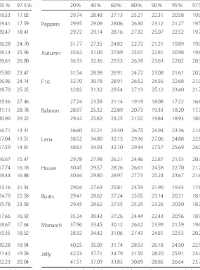
the Monte Carlo simulations for grayscale and color test images for several percentages of impulses are given in Tables 2 and 3. In each cell, the upper row represents the PSNR of the decision-based/adaptive median filter, the middle row represents the PSNR for the filter after sin-gle iteration of the BM3D algorithm, while the bottom row represents the PSNR after five iterations of the BM3D algorithm. Obviously, the largest gain is achieved with the first iteration of the BM3D algorithm while only moderate gain is achieved with additional four iterations.
The BM3D can be applied with similar improvement to all filters from this decision-based/adaptive median filter class [1, 3, 4, 14, 15]. Just to illustrate the improvement that is achieved in the last several years, we compare the obtained results with those from the initial paper [1] for test image “Lena” and several percentages of the salt-and-pepper noise. For example, the method from [1] for test image “Lena” corrupted by 20 % of impulses
achieves PSNR = 34.78 dB, while the proposed
Fig. 5Test trials for filtering color images.Left column- image “baboon;”right column- image “monarch.”First row- 80 % of impulses (a,d);second row- 90 % of impulses (b,e);third row- 95 % of impulses (c,f). For each image and noise percentage:upper left corner- corrupted image;upper right corner- filtered with decision-based/adaptive median filter;lower left corner- after single iteration with BM3D;lower right corner- after five iterations with BM3D
In order to quantify this gain, Fig. 7 presents the average improvement in the signal-to-noise ratio (ISNR) for all considered test images
ISNRi,j=10 log10 1
NM
n,m[h(j)(n,m)−f(n,m)]2
1
NM
n,m[h(i)(n,m)−f(n,m)]2
.
(5)
Three values are calculated: ISNR0,1 (improvement in
the SNR achieved for the first iteration), ISNR1,5
Fig. 6Enlarged part of test trials for test image “monarch.”First row- 80 % of impulses;second row- 90 % of impulses;third row- 95 % of impulses.
First column- original image;second column- filtered by the decision-based/adaptive median filter;third column- after single iteration with BM3D;
fourth column- after five iterations with BM3D
Table 2PSNR in filtering of grayscale images for various percentage of impulses
20 % 40 % 60 % 80 % 90 % 95 % 97.5 %
Cameraman
30.04 25.92 23.27 21.11 19.68 18.53 17.02 33.12 28.71 25.47 22.78 20.88 19.41 17.59 35.06 30.88 27.50 23.78 22.08 20.47 18.41
Mandi
38.95 34.78 32.15 29.90 28.00 26.28 24.70 40.61 37.38 35.22 32.98 30.55 28.13 25.96 40.51 37.16 34.76 45.14 30.49 28.61 26.80
Moon
40.95 36.03 32.71 30.34 28.30 25.80 23.47 42.97 39.17 36.03 32.98 30.25 26.96 24.14 42.79 39.17 36.63 34.19 32.30 28.70 25.25
Pout
43.94 39.01 36.05 33.58 31.30 29.36 27.46 44.26 41.03 38.25 36.33 33.56 31.11 28.78 43.85 40.33 36.97 34.10 32.16 30.90 29.22
Saturn
41.16 37.08 34.52 32.00 25.86 16.71 13.31 44.47 41.90 39.28 36.15 27.23 17.04 13.51 44.96 42.68 40.08 37.05 32.02 17.59 14.81
West Concord
28.82 24.49 21.80 19.68 18.02 16.67 15.47 30.31 26.53 24.00 21.60 19.50 17.74 16.18 30.41 46.57 24.01 21.37 19.84 18.44 16.88
Lena
36.94 32.26 29.44 26.87 25.00 23.16 21.54 39.46 35.51 32.81 29.76 27.31 24.79 22.58 39.49 35.70 32.68 29.78 27.74 25.78 23.58
Baboon
27.73 23.76 21.33 19.44 18.40 17.66 16.92 29.63 25.75 23.27 21.07 19.70 18.67 17.64 30.06 26.33 23.68 21.47 20.20 19.35 18.52
Clock
32.61 28.16 23.27 23.27 21.64 20.28 18.94 37.41 32.40 28.97 25.53 23.28 21.42 19.58 37.91 34.33 30.88 26.75 24.30 22.23 20.04
Upper row- decision-based/adaptive median filers;middle row- proposed scheme after single iteration by BM3D filter;bottom row- proposed scheme after five iterations by BM3D filter
Table 3PSNR in filtering of color images for various percentage of impulses
20 % 40 % 60 % 80 % 90 % 95 % 97.5 %
Peppers
29.74 28.48 27.13 25.21 22.31 20.58 19.01 29.95 29.09 28.06 26.30 23.12 21.27 19.52 29.72 29.14 28.16 27.32 25.07 22.52 19.71
Autumn
31.77 27.35 24.82 22.72 21.21 19.89 19.06 35.62 31.00 27.89 25.01 22.81 20.98 19.81 36.33 32.36 29.53 26.18 23.63 22.02 20.34
F16
31.54 28.98 26.91 24.72 23.08 21.61 20.28 32.70 30.78 28.91 26.52 24.56 22.68 21.00 32.82 31.32 29.54 27.13 25.12 23.40 21.79
Baboon
27.24 23.58 21.14 19.19 18.08 17.22 16.67 28.97 25.32 22.89 20.73 19.33 18.20 17.36 29.42 25.82 23.25 21.02 19.84 18.93 18.02
Lena
36.60 32.21 29.30 26.75 24.94 23.36 21.83 38.52 34.80 32.13 29.36 27.06 24.88 22.84 38.63 34.93 32.10 29.44 27.57 25.69 24.04
House
29.78 27.98 26.21 24.46 22.87 21.53 20.36 30.45 29.57 28.26 26.61 24.58 22.70 21.20 30.44 29.80 28.97 27.73 25.24 23.67 21.60
Boats
29.04 27.63 25.81 23.59 21.90 19.43 17.65 29.41 28.62 27.24 25.05 23.14 20.21 18.16 29.45 28.62 27.35 25.25 23.26 20.50 18.26
Monarch
35.24 30.43 27.26 24.44 22.43 20.56 18.98 37.96 33.45 30.12 26.62 23.99 21.59 19.65 38.32 34.42 31.06 27.43 24.81 22.53 20.29
Jelly
40.25 35.09 31.74 28.53 26.18 24.50 22.57 42.23 37.71 34.79 31.50 28.20 25.91 23.43 41.51 37.09 33.85 30.89 28.85 26.64 23.76
0 20 40 60 80 100 0 0.5 1 1.5 2 2.5 3 ISNR[dB]
% of impulses Additional 4 iterations First iteration Five iterations
Fig. 7Average improvement in the signal to noise ratio.Solid line -gain in the first iteration;dashed line- gain after five iterations;dotted line- gain in four iterations after the first one
impulses and gradually increases up to 0.8 dB for 90 % of impulses and after that decreases to 0.6 dB for 97.5 % of impulses. Total improvement is larger than 2 dB in the range of 20–93 % of impulses and in the entire considered range average ISNR is more than 1.2 dB with respect to the best decision-based/adaptive median filter.
It can be seen that four additional iterations of the BM3D filter brings relatively small gain; and if calculation complexity is critical, it can be used as a single iteration of the BM3D algorithm. Alternatively, some adaptation criterion can be employed to decide the number of the BM3D iterations. A simple criterion can be
10 log10 1
NM
n,m[h(i+1)(n,m)−x(n,m)]2
1
NM
n,m[h(i)(n,m)−x(n,m)]2
≤ε (6)
where it can be selectedε≈0.1 dB-0.2 dB.
In addition, we have compared considered filters using other quality measures of digital image filtering and reconstruction methods. In particular, we have considered the image enhancement factor (IEF) [23], structural simi-larity index (SSIM) [24], and edge-preserving index (EPI) [25]. The IEF is defined as
IEF=
1
NM[x(n,m)−f(n,m)]2
1
NM[h(n,m)−f(n,m)]2
. (7)
The SSIM is proposed in [24] as universal image qual-ity index between originalf(n,m)and corrupted and/or processed imageh(n,m):
SSIM= (2μhμf +c1)(2σhf +c2)
μ2
h+μ2f +c1 σh2+σf2+c2
(8)
where μh, μf are the mean values of corresponding
images,σh2,σf2are the image variances, while σhf is the
covariance:
μh=
1
NM n,mh(n,m) (9)
σ2
h =
1
NM n,m[h(n,m)−μh]
2 (10)
σhf =
1
NM n,m[h(n,m)−μh] [f(n,m)−μf] . (11)
Values c1 andc2are introduced to stabilize division for small denominator and commonly they are selected as c1 = 10−4fmax2 and c2 = 9 ·10−4fmax2 . Values closer to 1 correspond to higher structural similarity (better fil-tering). The EPI index is proposed in [25]. This index is very interesting here since our approach is developed to improve the shape of objects and in particular edges for images corrupted by high percentage of the salt-and-pepper noise. The EPI is defined as
EPI= σhHfH σ2
hHσ
2
fH
(12)
whereσh2
Handσ
2
fHare variances, whileσhHfHis the
covari-ance of highpass version of filteredhH(n,m)and original
fH(n,m)images. The Laplacian operator is used as a
high-pass filter for emphasizing high-frequency content, i.e., edges and details:
hH(n,m)=h(n−1,m)+h(n+1,m)+h(n,m+1)
+h(n,m−1)−4h(n,m).
(13)
Note that the EPI closer to 1 indicates better results as in the case of the SSIM. For brevity reasons, we have given only the results for test image “clock” in Table 4 while sim-ilar results as in Tables 2 and 3 are achieved for other test images.
Table 4Alternative filtering quality measures for grayscale color image “clock” (IEF, SSIM, and EPI)
20 % 40 % 60 % 80 % 90 % 95 % 97.5 %
IEF
128.57 91.87 73.80 61.95 46.19 33.81 27.59 396.87 244.12 156.46 107.60 66.77 42.51 32.21 497.86 358.55 254.93 158.33 88.00 52.42 37.76
SSIM
0.98 0.94 0.89 0.83 0.78 0.72 0.67 0.99 0.97 0.93 0.89 0.84 0.77 0.72 0.99 0.97 0.94 0.90 0.84 0.78 0.74
EPI
0.90 0.74 0.60 0.47 0.42 0.40 0.54 0.97 0.90 0.81 0.67 0.61 0.56 0.54 0.97 0.94 0.88 0.77 0.69 0.64 0.61
5 Conclusions
In this paper, we have proposed an application of the BM3D algorithm to the decision-based/adaptive median filter output for filtering salt-and-pepper noise. The BM3D filter with the proposed switching rule brings quite visible and measurable gain with respect to the decision-based/adaptive median filters. This research is a step in application of non-local and shaping filters to salt and pepper and other types of impulsive noises from digital images. Also, the proposed technique can be considered as an extension of the BM3D to challenging salt-and-pepper noise environment. Similar extensions and combi-nations of the BM3D with other filters are probably pos-sible but they remain for further research. In any case, we strongly believe that one of the most important directions in an actual digital image processing field is designing procedures for combining different, well-developed, fil-ters and their application to other problems outside of the originally considered area.
Competing interests
The author declares that he has no competing interests.
Acknowledgements
This research is supported in part by the Ministry of Science of Montenegro through the national project “Intelligent search techniques for parametric estimation in communication and power engineering” and by the EU with FP7 Project Foremont.
Received: 5 October 2015 Accepted: 3 March 2016
References
1. S Esakkirajan, T Veerkumar, AN Subramanyam, CH PremChand, Removal of high density salt and pepper noise through modified decision based unsymmetric trimmed median filter. IEEE Signal Process. Lett.18(5), 287–290 (2011)
2. RH Laskar, K Banerjee, D Basak, inProc. of International Conference on
Circuits, Power and Computing Technologies (ICCPCT). Removal of high
density salt and pepper noise from color images through variable window size, (2013), pp. 1132–1136. doi:10.1109/ICCPCT.2013.6528868 3. MM Rahman, F Ahmed, MI Jubair, SA Priom, IM Ziko, An enhanced
non-linear adaptive filtering technique for removing high density salt-and-pepper noise. Int. J. Comput. Appl.38(11), 7–12 (2012) 4. AR Telepatil, SA Patil, VP Parama, A survey on median filters for removal of
high density salt & pepper noise in noisy image. IOSR Journal of Electronics and communication Engineering (IOSR-JECE).1, 22–26 (2013). ISSN: 2278-2834, ISBN: 2278-8735
5. P Rodrigez, Total variation regularization algorithms for images corrupted with different noise models: A review. J. Electr. Comput. Eng.2013(Article ID 2170 21), 18
6. RH Chan, C-W Ho, M Nikolova, Salt-and-pepper noise removal by median-type noise detector and detail-preserving regularization. IEEE Trans. Image Process.14(10), 1479–1485 (2005)
7. R Lukac, B Smolka, KN Plataniotis, Sharpening vector median filters. Signal Process.87, 2085–2099 (2007)
8. J Astola, P Kuosmaneen,Fundamental of Nonlinear Digital Filtering. (CRC, Boca Raton, 1997)
9. S Zhang, MA Karim, A new impulse detector for switching median filters. IEEE Signal Process. Lett.9(11), 360–363 (2002)
10. KS Srinivasam, D Ebenezer, A new fast and efficient decision based algorithm for removal of high density impulse noise. IEEE Signal Process. Lett.14(3), 189–192 (2007)
11. M Nikolova, A variational approach to remove outliers and impulse noise. J. Math. Imaging Vis.20, 7 (2014)
12. R Lukac, B Smolka, KN Plataniotis, AN Venetsanopulos, Vector filtering for color imaging. IEEE Signal Process. Mag.22(1), 74–86 (2005)
13. S Morrilas, V Gregori, G Peris-Fajarnes, P Latorre. A fast impulsive noise color image filter using fuzzy metrics.Real-time Imaging.11(5-6), 421–428 (2005)
14. R Kaur, YS Randhawa, Comparative analysis of mean and median filter for high density salt and pepper noise removal. Int. J. Adv. Res. Comput. Sci. Softw. Eng.4(6), 1394–1401 (2014)
15. A Bhatia, inProc. of international conference on ITR. Decision based median filtering technique to remove salt and pepper noise in images
(Bhubaneswar, India, 2013), pp. 9–12. ISSN: 978-93-82702-26-9 16. K Dabov, A Foi, V Katkovnik, K Egiazarian, Image denoising by sparse 3D
transform-domain collaborative filtering. IEEE Trans. Image Process.16(8), 2080–2095 (2007)
17. A Buades, B Coll, JM Morel, inProc. of IEEE Computer Society Conference on
Computer Vision and Pattern Recognition. A non-local algorithm for image
denoising, vol. 2 (CVPR, 2005), pp. 60–65. doi:10.1109/CVPR.2005.38 18. J Zhang, R Xiong, C Zhao, Y Zhang, S Ma, W Gao, CONCOLOR: constrained
non-convex low-rank model for image deblocking. IEEE Trans. Image Process.25(3), 1246–1259 (2015)
19. EJ Candes, KJ Romberg, T Tao, Stable signal recovery from incomplete and inaccurate measurements. Commun. Pure Appl. Math.58(Np. 6), 1207–1223 (2006)
20. P Chatterjee, P Milanfar, Is denoising dead? IEEE Trans. Image Process.
19(4), 895–911 (2010)
21. S Sarjanoja,BM3D image denoising using heterogeneous computing
platforms. (University of Oulu, M.Sc.Thesis, 2015)
22. M Lebrun, An analysis and implementation of the BM3D image denoising method. Image Process Line.2, 175–213 (2012). http://dx.doi.org/10. 5201/ipol.2012.l-bm3d
23. S Malviya, H Ahmia, Image enhancement using improved mean filter at low and high noise density. Int. J. Emerging Eng. Res. Technol.2(3), 45–52 (2014)
24. Z Wang, AC Bovik, HR Sheikh, EP Simoncelli, Image quality assessment: from error visibility to structural similarity. IEEE Trans. Image Process.
13(4), 600–612 (2004)
25. F Sattar, L Floreby, G Salomonsson, B Lovstrom, Image enhancement based on a nonlinear multiscale method. IEEE Trans. Image Process.6(6), 888–895 (1997)
Submit your manuscript to a
journal and benefi t from:
7Convenient online submission
7 Rigorous peer review
7Immediate publication on acceptance
7 Open access: articles freely available online
7High visibility within the fi eld
7 Retaining the copyright to your article