DeepHist: Towards a Deep Learning-based
Computational History of Trends in the NIPS
Amna Dridi
Birmingham City University, UK Email: [email protected]
Mohamed Medhat Gaber
Birmingham City University, UK Email: [email protected]
R. Muhammad Atif Azad
Birmingham City University, UK Email: [email protected]
Jagdev Bhogal
Birmingham City University, UK Email: [email protected]
Abstract—Research in analysis of big scholarly data has increased in the recent past and it aims to understand research dynamics and forecast research trends. The ultimate objective in this research is to design and implement novel and scalable methods for extracting knowledge and computational history. While citations are highly used to identify emerging/rising re-search topics, they can take months or even years to stabilise enough to reveal research trends. Consequently, it is necessary to develop faster yet accurate methods for trend analysis and computational history that dig into content and semantics of an article. Therefore, this paper aims to conduct a fine-grained content analysis of scientific corpora from the domain of Ma-chine Learning. This analysis uses DeepHist, a deep learning-based computational history approach; the approach relies on a dynamic word embedding that aims to represent words with low-dimensional vectors computed by deep neural networks. The scientific corpora come from 5991 publications from Neural Information Processing Systems (NIPS) conference between1987 and 2015 which are divided into six 5-year timespans. The analysis of these corpora generates visualisations produced by applying t-distributed stochastic neighbor embedding (t-SNE) for dimensionality reduction. The qualitative and quantitative study reported here reveals the evolution of the prominent Machine Learning keywords; this evolution supports the popularity of current research topics in the field. This support is evident given how well the popularity of the detected keywords correlates with the citation counts received by their corresponding papers: Spearman’s positive correlation is 100%. With such a strong result, this work evidences the utility of deep learning techniques for determining the computational history of science.
I. INTRODUCTION
The abundance of scholarly data sources like digital libraries and academic social networks has enabled big scholarly data analysis. With this data it is now possible to develop a com-putational history of science and consequently ask interesting questions such as what scientific trends are emerging in a given scientific field.
Many researchers have realised the importance of mining scholarly data to understand the dynamics of science. Gen-erally, tracking the dynamics of science is highly related to revealing hidden trends within the vast quantity of available resources. Hence, trend analysis has been popular in the research community of scholarly data analysis [1] that looks for popular keywords.
Commonly the detection of evolving scientifickeywordsor
trends has widely relied on citation analysis; however, this analysis is not fool proof. While citation counts can signify the importance of scientific work, these counts may also grow for non-scientific reasons [2]. Instead, there can be other interesting papers – termed assleeping beauties [3] – which do not get cited much for several years after publication, but then unexpectedly start getting cited.
For the reasons cited above and the fact that citation-based approaches fail to dig into the paper content which could lead to a more accurate trend detection, some emerging researchers [4], [5] have followed a particular direction in computational history which is the use of topic models to analyse the rise and fall of research topics and accordingly the progress of science.
Going beyond the topic models that capture document level associations between words, our aim in this paper is to learn
word embeddingsacross time in scientific corpora due to the ability of word embeddings to detect very local associations. For instance, it has been shown that word embeddings can suc-cessfully capture both the semantic and the syntactic features of words [6]. They can complement topic models, or stand alone as an approach to building a computational history of science.
To do so, this paper introduces DeepHist, a deep-learning based approach to computational history that uses dynamic word embedding in order to study the semantic shifts of words and consequently detect the evolving scientific keywords; in this paper, wordsand keywords are used interchangeably. To detect the semantic shift of words, we build asimilarity matrix
that records similarity between frequent keywords embedding vectors over each timespan. Then, based on these matrices, we create anacceleration matrix that computes theacceleration
of various keywords over subsequent timespans in order to detect fast converging keywords. The acceleration represents the difference in similarities between keywords over two successive timespans. The subject area used in this work is Machine Learning. This choice owes both to the authors’ background in this subject area, and the fact that Machine Learning has enjoyed notable successes in the recent years.
5991 publications from the NIPS conference proceedings between the years 1987 and 2015 that we divided into six timespans of 5-years each. For evaluating the effectiveness of our embeddings in detecting emerging scientific keywords, we adopt both qualitative and quantitative methods.
• Qualitatively, we illustrate the advantages of dynamic embeddings that show the evolving scientific keywords in the area ofMachine Learningfor each timespan by plot-ting keyword vectors after reducing their dimensions with
t-distributed stochastic neighbor embedding (t-SNE) [7]. All t-SNE visualisations show that our embeddings are able to illustrate the fast acceleration between the emerg-ing scientific keywords.
• Quantitatively, to validate our approach against the com-monly used citation analysis approach, we collect the citation counts of NIPS publications having detected the emerging keywords in their titles, track the citation evolution over time and compute its correlation with the obtained similarities captured by our embeddings. The ex-perimental results show the effectiveness of our approach that was able to detect that the keywords “neural” and
“learning” were getting similar across time and rising by 70% in similarity in the timespan 2007-2011 when the emerging keyword“deep learning”started to flourish as a neural-based learning. Interestingly, our approach succeeded to achieve a100%positive correlation between the citation counts and the similarities returned by our embeddings.
The rest of the paper is organised as follows. Section II details our DeepHist methodology and how we employ word embeddings, namelyskip-gram modelto detect rising scientific keywords in the area of Machine Learning. Section III de-scribes the NIPS dataset we have used, presents and discusses the obtained results. A summary of existing work is briefly presented in Section IV. Finally, in section V we conclude the paper and draw future directions.
II. DEEPHIST
This study introduces a deep-learning based computational history (DeepHist) that tracks rise or evolution of scientific keywords and hence the evolution of Machine Learning itself. Accordingly, we adopt adynamic word embeddingstechnique to learn word vectors in a temporal fashion, in order to capture words that get geometrically closer, and hence reveal emerging keywords. The skip-gram (SG)neural network architecture of
word2vec embedding model [8] is used in this paper as it consistently performed better than thecontinuous bag of words (CBOW)architecture.
A. Skip-Gram Neural Network Model
To learn high-quality distributed vector representations, the
skip-gram (SG) neural network model was introduced by Mikolov et al. [6]; SG can successfully capture both the semantic and the syntactic word regularities [6].
1) Notation: We consider the corpora of NIPS pub-lications collected across time (1987-2015). Formally, P = (P1, . . . ,PT) where each Pt|t=1, . . . ,T is the corpus of all publications in the tth timespan, and V = (word1, . . . ,wordN) is the vocabulary that consists of
N words present in the corporaP at any point in time; thus, it is likely for somewordi ∈V to not appear at all in some Pt. V comprises of both emerging and dying words as they typically occur in scientific corpora.
Given this time-tagged scientific corpora, our goal is to find a dense, low-dimensional vector representation uwordi(t)∈R
d,d |V|for each wordword
i ∈V and each timespant =1, . . . ,T; d is thedimensionality or the length of the word vectors.Minput is the matrix of sizeN ×d that
represents the input to hidden layer connections with each row representing a vocabulary wordwordi,i =1, . . . ,N, and
Moutput is the matrix of size d×N that describes the
connections from hidden layer to output layer where each column ofMoutput represents a word wordi ∈V.
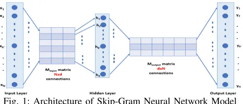
2) Model: Skip-gram modeluses a single hidden layer, fully connected neural network as simplified in Figure 1.
Fig. 1: Architecture of Skip-Gram Neural Network Model
The neurons in the hidden layer are all linear neurons. The input layer is set to have as many neurons as there are words in the vocabulary, i.e., N. The hidden layer size is set to the dimensionality d of the resulting word vectors. The size of the output layer is same as the input layer and they are represented respectively by the matrices Minput |N×d| and
Moutput |d×N|. The input to the network is encoded using“1
-out of -N” representation, meaning that only one input line is set to1 and the rest of the input lines are set to zero.
The main idea ofskip-gramis to predict thecontextgiven a wordwordi. Note that thecontextis a window aroundwordi
of maximum sizeL that represents the span of words in the text; the span runs both backwards and forwards when iterating through the words during model training.
Since the goal ofskip-gram modelis to produce probabili-ties for the words in a context (context words) in the output layer given a word wordi,Prob(wordcontext|wordi)i=1,...,N, the model needs the neuron outputs in the output layer to sum to one. Word2vec achieves this by converting activation values of output layer to probabilities using the softmax function. Thus, the output of the k0-th neuron is computed by the following expression:
yk0 =P rob(wordcontext|wordi) =
exp(activation(k0))
PN
B. Skip-Gram Hyperparametrisation
Skip-Gram model depends on several hyperparameters; some of them crucially impact the quality of embeddings, especiallyvector dimensionalityandcontext window. Despite that, the majority of applications that used word embeddings as features computed their vector representations with a default or arbitrary choice of hyperparameters.
Since the optimal hyperparameters values are known to be often data and task dependent, we proposed a domain-specific approach to hyperparametrisation [9] for skip-gram; the domain is scientific and specifically concerns Machine Learning literature. The approach uses the stability of k-nearest neighbors (k-NN) of word vectors as the objective to measure while learning word2vec hyperparameters.
Stability is an important aspect of a learning algorithm. It has been widely used in clustering problems [10] to assess the quality of a clustering algorithm. Also, it has been applied in high-dimensional regression [11] for training parameter selection. Since word embedding produces high-dimensional word representations that can be organised into word clusters, we applied the k-NN algorithm to tune the hyperparameters of skip-gram model until the k-NN clustering is stable.k-NN clusters similar words based on their cosine similarities.
The basic idea of word embedding stability is the following: the quality of embedding inevitably depends on tuning hyper-parameters defined previously, namely vector dimensionality
andcontext window. If we choose accurate values of the tuning hyperparameters, then we expect to findkwords from different embeddings that are similar to a target wordwordi.
Thek-NN embedding stability approach follows four steps: 1) Fix one hyperparameter at the beginning (choose the
default value for example).
2) Tune the second hyperparameter by trying different val-ues and training the model for each value.
3) Compute word similarities after each training and define
k-nearest neighboring words.
4) Repeat steps 2 and 3 for the second hyperparameter to be tuned after fixing the first one (step1) to the optimal value already obtained.
The k-NN stabilityis defined as the overlap rate of similar words resulting from two different embeddings.
stability= S
wordi
Eh ∩ S
wordi Eh0
k ×100
where SEh and SEh0 are two sets of words that are similar
to a target wordwordi but were produced from two different embeddingsEhandEh0 with different hyperparameter values.
k is the number of nearest neighbors towordi given by the cosine similarity. In this study, k is set to 5. This choice is motivated by our aim to keep the word similarities as fine-grained as possible in order to evaluate the quality of skip-gram model within scientific text.
In our previous work [9], we showed that the optimal hy-perparameters values are 200and6for vector dimensionality
d and the context window respectively for the NIPS corpora
we are using. Therefore, the skip-gram model is tuned with these hyperparameters in this work.
C. Dynamic Skip-Gram Model
To track the dynamism of skip-gram embeddings and mea-sure the accelerations of potential emerging keywords, we pro-pose to create a similarity matrixMij(t)of size |V0| × |V0|, V0⊂V, for each timespantthat corresponds to the distance metric between two words. Note that V0 represent the set of frequent keywords. All distances between two words wordi
(wi) andwordj (wj) are calculated by the cosine similarity
between embedding vectors uwi and uwj. Recall that Mij(t) is a symmetric matrix.
sim(wi, wj) =cosine(uwi, uwj) = uwi·uwj kuwik · kuwjk
Then, we generate an acceleration matrix Aij of size |V00| × |V00|, V00=Vt0∩Vt0+1, that corresponds to the ac-celeration between two words wi and wj from t to t+ 1. The acceleration between two wordswi andwj acceleration
(wi, wj)is defined as follows.
acceleration(wi, wj) =sim(wi, wj)t+1−sim(wi, wj)t
Two keywords are defined as emerging keywords if their acceleration over two timespanst andt+ 1is greater than a defined thresholdθ. We setθto the acceleration average over
T, θ = T1 PT t=1
1
|V00|
P
i,jacceleration(wi, wj), wi and wj
are belongingV00.
III. EXPERIMENTS
To analyse the computational history in the domain of Machine Learning, we evaluate our proposed approach on a time-stamped text corpora extracted from NIPS publications. NIPS has been chosen as one of the top Machine Learning conferences in the world that covers topics fromdeep learning
and computer vision to cognitive science and reinforcement learning. We demonstrate that our approach finds acceleration between trending keywords over time. This allows us to track the evolving scientific discovery in the field by following dynamic embeddings. The dynamic embedding is used to define the acceleration of various keywords over subsequent timespans in order to detect fast emerging keywords and subsequently emerging trends.
A. NIPS Dataset and Preprocessing
The data used for this analysis is a set of 5991 papers published between 1987 and 2015. The dataset is publicly available on Kaggle1 and contains information about papers, authors and the relation between papers and authors.
The data set was first preprocessed. Data preprocessing consists of two steps: (i) the removal of stop words from the text using Stanford NLP stop word list2 and a list of 170 academic stop words that we defined from common
1https://www.kaggle.com/benhamner/nips-2015-papers/data
2https://github.com/stanfordnlp/CoreNLP/blob/master/data/edu/stanford/
academic vocabulary like “introduction, abstract, table, figure, etc.”; and (ii) the construction of bag of words where words are either unigrams used for standard word2vec training or
bigramsextracted withword2phrase.Word2phraseattempts to learn phrases by progressively joining adjacent pairs of words with a ‘ ’ character [8]. It is used as a method for corpus augmentation.
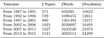
To study the temporal evolution of the trends in Machine Learning by tracking emerging scientific keywords, we divided the NIPS publications between 1987 and 2015 into six 5-years timespan; however, the last timespan is 4-years long. Therefore, the skip-gram embeddings of the year t0 will contain a snapshot of the interactions between keywords in the timespan (t0−4, t0). For instance, an embedding of the year 2005 will describe how the word embeddings of keywords developed in the years 2001 to 2005. The length of the timespan is based on the study performed by Hoonloret al.[1] on evolving Computer Science research. That investigation showed that the average length of the evolutionary chain is4.5 years. This choice was also tested successfully by Salatinoet al. [5]. The statistics of the dataset are given in Table I.
Table I shows a positive trend in the evolution of the number of papers per 5-years over the 1987-2015 study period. The average 5-annual growth rate is22%, rising to29.71%in the timespan 2007-2011.
TABLE I: Statistics of NIPS dataset
Timespan ]Papers ]Words ]Vocabulary
From1987to1991 571 859293 10823
From1992to1996 729 1096455 12651
From1997to2001 800 1301492 13471
From2002to2006 1023 2020697 16493
From2007to2011 1327 3243526 21074
From2012to2015 1541 4002513 24299
B. Results and Discussion
We evaluate the use of dynamic word embeddings on the content analysis of Machine Learning scientific publications and their impact on the evolution of the main streams of Machine Learning keywords. To do so, NIPS publications published between1987and2015and divided into six5-years timespans, have been used.
Our goal of these experiments is two-fold.
1) We aim to evaluate whether our training data with dynamic word embedding representations derived from word2vec skip-gram model (where word is not only a unigram, but can also be a bigram) is useful for tracking trends and emerging keywords for theMachine Learning
domain.
2) We want to study the concordance between our deep learning trend analysis method, and the citation-based analysis method, commonly used in the literature. To generate embeddings, we started with a text analysis step. For each timespan t, we created a corpus Pt of all publications published during this time period. Then, after removing stop words, we performed term frequency statistics
Fig. 2: Frequencies of “deep”, “neural” and “learning” over time
on unique words of the vocabulary based on two types of bag-of-words: unigrams and bigrams, in order to study the evolving keywords over time based on their frequencies. Early findings [12] illustrated that word frequency itself is correlated with the success of the keywords historically. We explored the relation between dynamism and frequency change in order to gain insights into emerging keywords in the area of Machine Learning.
By examining the20most frequent unigrams and bigrams from the NIPS publications over the six timespans covering a total of 28 years, it was clear that the frequencies of n -grams evolve considerably over time. Interestingly, we found that the frequencies of some words (unigrams and bigrams) increase by approximately the same rate in specific timespans. For example, we found that the frequencies of “neural”
and “learning” rose simultaneously between the timespan (1987-1991) and the timespan (1992-1996); this indicates that learning in this time period primarily relied on neural compu-tation. Interestingly, this observation is justified by bigrams. For instance, we noticed increasing frequencies of “neural-networks”,“reinforcement-learning”and“machine-learning”
in the next timespans (1997-2001) and (2007-2011).
It seems that as the word usage increases together, these words merge and become emerging keywords. To test the effectiveness of this observation, and assuming that “deep-learning” is the emerging trend or keyword in the area of
Machine Learning in the last few years while our dataset is limited to only 2015 publications, we tried to investigate an intriguing prediction based on the frequencies that we have. Considering that “deep learning” is learning based on neural computation, we tracked the frequencies of“learning”,
“neural”and“deep”over time. Recall that“deep”and“deep learning”do not appear on top-100words in all timespans. We notice that suddenly the frequency of“deep”had a jump in the timespan (2012-2015) that presents the period of emergence ofdeep learning. Fig. 2 shows how“deep learning”as neural learning appears over this 28-year period. The frequency of “deep” remained steady, basically null (equal to 19 on the timespan 1997-2001) until 2005 where it started to rise slightly. Then, it rose dramatically to 2913 in the timespan 2012-2015. In this last time period, the frequencies of the three unigrams rose in a parallel way which justifies their concordance.
cor-pora. We can automatically detect keywords that accelerate significantly to get close over time.
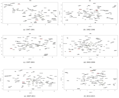
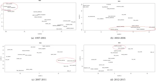
Fig. 3 shows t-SNE representations of the six timespans con-sidering bag-of-unigrams, while Fig. 4 shows t-SNE represen-tations of the last four timespans considering bag-of-bigrams. t-SNE takes the200dimensions via word2vec vectors, then re-duces them down to2-dimensional (x,y) coordinate pairs. The idea is to keep similar words close together on the plane, while maximising the distance between dissimilar words (words are unigrams or bigrams). We plotted the2-D t-SNE projection of each unigram’s and bigram’s temporal embedding across time. For visualisation purposes, we plotted t-SNE representations of only top-100and top-20most frequent unigrams and bigrams respectively.
We pick2unigrams of interest in the t-SNE representations related to unigrams: “neural” and “learning”. In all visu-alisations, the embeddings illustrate significant acceleration between the two unigrams. As a matter of fact, their similarity (cosine similarity) is increasing over time. For instance, it increased from 0.0657 in the second timespan (1992-1992) to 0.2235 in the fifth timespan (2007-2011). Table II shows an increase of70%in similarity, which suggests thatlearning
was increasingly based on neural computation/networks and consequently the combination of these unigrams could lead to emerging keywords.
TABLE II: Temporal similarity between “neural” and “learn-ing”
87-91 92-96 97-01 02-06 07-11 12-15
0.1657 0.0657 0.09650 0.1806 0.2235 0.1994
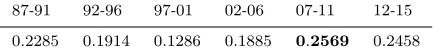
Knowing that the unigram “deep” is used together with the semantics ofneural computation/networksand considering that “deep” is not represented in top-100 frequent unigrams, we computed the similarity between “deep”and “learning”
to verify if“deep”and“neural”get similarly close to “learn-ing”over time. Table III shows that like“neural”,“deep”gets close to“learning”chronologically; in fact, it gets even closer to “learning” with a similarity consistently higher than that of “neural” over all the timespans. These findings from the embeddings agree with the statistics previously calculated on term frequencies and support the effectiveness of our approach. TABLE III: Temporal similarity between “deep” and “learn-ing”
87-91 92-96 97-01 02-06 07-11 12-15
0.2285 0.1914 0.1286 0.1885 0.2569 0.2458
Fig. 4 shows t-SNE representations of the last four times-pans considering bag-of-bigrams. We plotted the 2-D t-SNE projection of each bigram’s temporal embedding across time. For visualisation purposes, we plotted t-SNE representations of only top-20most frequent bigrams.
To be consistent, we analyse t-SNE visualisations for bigrams by choosing bigrams similar to the uni-grams of interest. The biuni-grams of interest are:
“neural-networks”, “neural-computation”, “reinforcement-learning”
and “machine-learning”. As we plotted only the top-20 bigrams, not all the selected bigrams appear in all visu-alisations. Hence, we focus only on visualisations of the last four timespans as they mostly contain the bigrams of interest. In Fig. 4(a) (third timespan: 1997-2001), we see the bigram “reinforcement-learning” and its neighbor-hood derived from“neural”. i.e. “neural-network”, “neural-networks” and “neural-computation”. This is: (i) semanti-cally significant as “reinforcement-learning”by definition is called neuro-dynamic programming and needs incremental
“neural networks”; and (ii) proved by similarity as the latter reaches its peak by 0.9998 during this time period. Like-wise, the similarity between“machine-learning”and “neural-networks” peaks at almost the same value of 0.9997 while
“machine-learning” is not represented in the figure that shows only the 20 most frequent bigrams. This also indi-cates that “reinforcement-learning” was used as “machine-learning” during this time period; in fact, the similarity between“reinforcement-learning”and“machine-learning”is equal to0.9994.
One timespan later (2002-2006) (Fig. 4(b)), “machine-learning” appears and its similarity to “neural-networks”
drops significantly to 0.8686. This shows that “machine learning” started to flourish towards the end of1990s as an independent topic while “reinforcement learning” remained linked to“neural computation/networks”.
In the fifth timespan (2007-2011) (Fig. 4(c)) “neural-networks/computation” does not appear in the top-20 fquent bigrams. However, this timespan highlights the re-approximation between “machine learning” and “reinforce-ment learning” that incorporates “neural networks”. This is insightful as it shows how“machine learning”is increasingly related to“neural networks/computation”.
The last timespan (2012-2015) (Fig. 4(d)) also shows that
“machine learning” is geometrically very close to “neural networks” that re-appeared, while “reinforcement learning”
disappeared from the top-20bigrams. This shows that possibly
“machine learning” increasingly implies “neural networks”
just as“reinforcement learning” did earlier.
Based on the findings of bigrams embedding and knowing that “deep-learning” was the emerging keyword in the last few years, we computed the similarity between “machine-learning”and“deep-learning” and we found that it is equal to 0.8716 while “deep-learning” does not exist in previ-ous timespan-vocabularies. Consequently, we can assume that
“deep-learning”is the keyword that emerged from the conver-gence between“machine-learning”and“neural-networks”.
(a)1987-1991 (b)1992-1996
(c)1997-2001 (d)2002-2006
(e)2007-2011 (f)2012-2015
Fig. 3: t-SNE of top 100 unigrams of all timespans;the overlapping keywords – horizontally from left to right, and then vertically from top to bottom – are as follows: in 3(a):{“distributed, parallel”, “probability, distribution”, “initial, random”}, in 3(b):{“problem, task”, “distribution, probability”, “unit, layer”}, in 3(c):{“theorem, bound”, “analysis, independant”, “simple, similar”}, in 3(e):{“optimization, normalization”, “dataset, images”, “prediction, classification”, “posterior, distribution”}, and in 3(f):{“training, testing”, “model, architecture”, “prediction, classification”, “min, max”, “problem, task”, “performance, accuracy”, “large, small”}
contain the cosine similarity between the embedding vectors of every two keywords.
After creating the similarity matrices, we generated the
acceleration matrix as described in II-C. We computed the average acceleration θ that corresponds to the average over all the selected keywords. θ was negative and equal to −0.0656. Overall, almost all accelerations are negative but some of them were speeding up. For instance, the couple of bigrams{“neural-networks”, “reinforcement-learning”}have an acceleration of −0.011, which is much greater than the averageθ. Interestingly, we found that the acceleration of the couple of bigrams{“neural-networks”, “machine-learning”} is positive and equal to0.0094. Respectively, the acceleration of the couple of unigrams{“neural”, “learning”}is positive
and has a value of 0.02. Both of them have an acceleration much greater than the average (θ). These findings support the previous ones and show that neural-based learning was speeding up over time. Similar to previous investigations about the emergence of “deep learning”, we computed the acceleration of two unigrams {“deep”, “learning”} and two bigrams {“neural-network”, “deep-learning”}. Their values are respectively 0.0034 and 0.1649, showing a substantial speed up over the averageθ.
(a)1997-2001 (b)2002-2006
(c)2007-2011 (d)2012-2015
Fig. 4: t-SNE of top 20bigrams of the four timespans between 1997and2015
the extent to which citation analysis supports the findings of DeepHist. To do so, we retrieved academic citations of all the NIPS publications in our dataset (1987 to 2015) using the Public or Perishsoftware3 that uses Google Scholar4 to obtain the raw citations.
For consistency, we tracked the citation counts of publi-cations with previously selected frequent keywords (the key-words of interest we picked in the qualitative analysis) over time such that in each timespan we noted the citation counts of the publications that used the picked keywords in their titles; we assume that the title plays a pivotal role in communicating research.
We compare the acceleration of citation counts of publica-tions mentioning the keywords of interest in their titles with the acceleration of similarities of these keywords that our embeddings return over all timespans.Spearman’s correlation coefficient ρ has been used to measure the strength and direction of association between these two variables. ρ is defined as following:
ρ=
P
s(xs−x¯)(ys−y¯) pP
s(xs−x¯)2 P
s(ys−y¯)2
wheresis the paired score(citation count, similarity),x
andycorrespond to the citations counts and similarity values, ¯
xandy¯correspond respectively to the mean of citations counts and the mean of similarity values.
3https://harzing.com/resources/publish-or-perish 4https://scholar.google.com/
Spearman’s correlation coefficient has been computed for all the pairs of picked keywords. Interestingly, we found that 100%of cases have a positive correlation with an average of 0.422.67%of these correlations are strong withρcoefficient greater than 0.6.
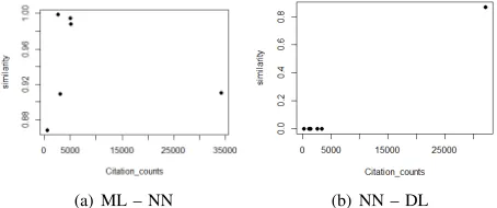
Fig. 5(a) and Fig. 5(b) show the relationships between the citation counts and the similarities of the keywords of interest“machine-learning – neural-networks (ML – NN)”and
“neural-networks – deep-learning (NN – DL)” respectively. Fig. 5(a) has Spearman’s correlation coefficient ρ equal to 0.2. If we do not consider the last point where the similarity between“machine-learning”and“neural-networks” dropped in the timespan (2002-2006), ρ coefficient is much higher and equal to 0.9. This observation could be justified by the fact that “machine learning” started to flourish towards the end of 1990s as an independent topic which justifies the decrease in similarity with “neural-networks”. Overall, this new finding confirms our previous findings stating that
learningwas correlated toneural networksover time. Fig. 5(b) hasρcoefficient equal to0.654. This result perfectly matches with our previous findings where the citation count was slightly small in the first four timespans. Then, suddenly it rose dramatically to reach 3223 in the last timespan (2012-2015). A significant rise of these citation counts is clearly seen which goes with the increase in the similarity and the acceleration previously detailed, and shows that “learning”
the assumption that “deep-learning” is now the trend.
(a) ML – NN (b) NN – DL
Fig. 5: Spearman’s coefficient plot of (ML – NN) and (NN – DL)
These findings resulting from citation counts support the effectiveness of our approach based on dynamic word embed-dings in discovering rising keywords in the domain of Machine Learning.
IV. RELATEDWORK
The emerging research addressing trend analysis can be categorized into three categories: bibliometrics-based ap-proaches [13] that are based on social network analysis and citation analysis; content-based approaches [14] that treat entities – essentially keywords – reflecting the paper con-tent [14]; and hybrid approaches [15] that combine both citation and content. These approaches dealing with trend analysis have been applied to a wide range of disciplines such as business [16], computer science [1], [15],etc.In this paper, we concentrate on an area withinComputer Science (CS).
While we are not aware of previous works on predicting research trends in CS by drilling into paper content and following a fine-grained content analysis, there are few works addressing related research problems in investigating general publication trends, citation trends and evolution of research ar-eas following a coarse-grained analysis. For instance, Hoonlor et al. [1] analysed data on proposals for grants supported by the U.S National Foundation and on CS publications in the ACM Digital Library and IEEE Xplore Digital Library using sequence mining and bursty word detection. Similarly, Hou et al. revealed the evolution of research topics between 2009 and 2016 using the timeline knowledge map through Document-Citation Analysis (DCA). In the same context, Effendy and Yap [15] performed trend analysis using the Microsoft Academic Graph (MAG) dataset. Both the above approaches to trend analysis in CS focus on citation analysis which fails to dig into the paper content and takes time to reveal trends.
V. CONCLUSIONS
We offer DeepHist, a deep learning-based approach for computational history and apply it to the NIPS publications to produce insights about the field of Machine Learningand track the evolution of new trends.
This work addressed this challenge in an innovative way by bringing together qualitative and quantitative analysis of NIPS publications during the time period1987-2015. Both analyses
drilled into the paper content by computing and visualising temporal keyword embeddings over six 5-years timespans. We explored the similarity between keywords by embedding vectors to create a similarity matrix of frequent keywords. Then, based on this matrix we created an acceleration matrix that reports the acceleration between keywords over time in order to capture the speeding up keywords that may result in a trending keyword. Our results were able to detect that “deep-learning” was the convergence between “machine-learning”
and “neural-networks”. Our approach has been validated against citation count analysis, and its effectiveness has been demonstrated.
As future work, we plan to generalise our approach on different research areas such asphysics, biologyor medicine
where it would be interesting to see whether a novel treatment or a certain combination of drugs for cancer is beginning to rise. Furthermore, we plan to expand the embedding technique with more text analysis techniques that explore the semantics of paper content and help to detect emerging topics such as
topic modeling.
REFERENCES
[1] A. Hoonlor, B. K. Szymanski, and M. J. Zaki, “Trends in computer science research,”Commun. ACM, vol. 56, no. 10, pp. 74–83, 2013. [2] L. Bornmann and H. Daniel, “What do citation counts measure? a review
of studies on citing behavior,”Documentation, vol. 64, no. 1, pp. 45–80, 2008.
[3] R. Dey, A. Roy, T. Chakraborty, and S. Ghosh, “Sleeping beauties in computer science: characterization and early identification,” Scientomet-rics, vol. 113, no. 3, pp. 1645–1663, 2017.
[4] A. Anderson, D. McFarland, and D. Jurafsky, “Towards a computational history of the acl: 1980-2008,” in ACL-2012 Special Workshop on
Rediscovering 50 Years of Discoveries, 2012, pp. 13–21.
[5] A. A. Salatino, F. Osborne, and E. Motta, “How are topics born? understanding the research dynamics preceding the emergence of new areas,”PeerJ Computer Science, vol. 3, p. e119, 2017.
[6] T. Mikolov, W.-t. Yih, and G. Zweig, “Linguistic regularities in contin-uous space word representations.” inNAACL-HLT, 2013, pp. 746–751. [7] L. van der Maaten and G. Hinton, “Visualizing data using t-SNE,”
Journal of Machine Learning Research, vol. 9, pp. 2579–2605, 2008.
[8] T. Mikolov, I. Sutskever, K. Chen, G. S. Corrado, and J. Dean, “Distributed representations of words and phrases and their composi-tionality,” inNIPS, 2013, pp. 3111–3119.
[9] A. Dridi, M. M. Gaber, R. M. A. Azad, and J. Bhogal, “k-nn embed-ding stability for word2vec hyper-parametrisation in scientific text,” in
Discovery Science, 2018, pp. 328–343.
[10] A. Rinaldo, A. Singh, R. Nugent, and L. Wasserman, “Stability of density-based clustering,” Journal of Machine Learning Research, vol. 13, no. 1, pp. 905–948, 2012.
[11] Nicolai Meinshausen and Peter Bhlmann, “Stability selection,” Royal
Statistical Society, vol. 72, no. 4, pp. 417–473, 2010.
[12] E. Lieberman, J.-B. Michel, J. Jackson, T. Tang, and M. A. Nowak, “Quantifying the evolutionary dynamics of language,”Nature, vol. 449, no. 7163, pp. 713–716, 2007.
[13] J. Hou, X. Yang, and C. Chen, “Emerging trends and new developments in information science: a document co-citation analysis (2009–2016),”
Scientometrics, vol. 115, no. 2, pp. 869–892, 2018.
[14] C. Weismayer and I. Pezenka, “Identifying emerging research fields: a longitudinal latent semantic keyword analysis,”Scientometrics, vol. 113, no. 3, pp. 1757–1785, 2017.
[15] S. Effendy and R. H. Yap, “Analysing trends in computer science research: A preliminary study using the microsoft academic graph,” in
WWW, 2017, pp. 1245–1250.