Patron: Her Majesty The Queen Rothamsted Research Harpenden, Herts, AL5 2JQ
Telephone: +44 (0)1582 763133 Web: http://www.rothamsted.ac.uk/
Rothamsted Research is a Company Limited by Guarantee Registered Office: as above. Registered in England No. 2393175. Registered Charity No. 802038. VAT No. 197 4201 51. Founded in 1843 by John Bennet Lawes.
Rothamsted Repository Download
A - Papers appearing in refereed journals
Puche, N., Senapati, N., Flechard, R., Klumpp, K., Kirschbaum, M. U. F.
and Chabbi, A. 2019. Modeling Carbon and Water Fluxes of Managed
Grasslands: Comparing Flux Variability and Net Carbon Budgets
between Grazed and Mowed Systems. Agronomy. 9 (4), p. 183.
The publisher's version can be accessed at:
•
https://dx.doi.org/10.3390/agronomy9040183
•
https://www.mdpi.com/2073-4395/9/4/183
The output can be accessed at: https://repository.rothamsted.ac.uk/item/8wv48.
© 10 April 2019, Rothamsted Research. Licensed under the Creative Commons CC BY.
Article
Modeling Carbon and Water Fluxes of Managed
Grasslands: Comparing Flux Variability and Net
Carbon Budgets between Grazed and Mowed Systems
Nicolas Puche1, Nimai Senapati2 , Christophe R. Flechard3, Katia Klumpp4 , Miko U.F. Kirschbaum5 and Abad Chabbi1,6,*
1 INRA, Versailles-Grignon, UMR ECOSYS, Bâtiment EGER, 78850 Thiverval-Grignon, France;
2 Rothamsted Research, Department of Plant Sciences, West Common, Harpenden, Herts AL5 2JQ, UK;
3 INRA UMR 1069 SAS, 65 rue de Saint-Brieuc, 35042 Rennes, France; [email protected]
4 INRA, VetAgro Sup, UMR 874 Ecosystème Prairial, 63100 Clermont Ferrand, France; [email protected] 5 Manaaki Whenua—Landcare Research, Private Bag 11052, Palmerston North 4442, New Zealand;
6 INRA, Centre de recherche Nouvelle-Aquitaine-Poitiers, URP3F, 86600 Lusignan, France * Correspondence: [email protected]; Tel.:+33-(0)1-3081-5289 or+33-(0)6-8280-0285
Received: 2 March 2019; Accepted: 7 April 2019; Published: 10 April 2019
Abstract: The CenW ecosystem model simulates carbon, water, and nitrogen cycles following ecophysiological processes and management practices on a daily basis. We tested and evaluated the model using five years eddy covariance measurements from two adjacent but differently managed grasslands in France. The data were used to independently parameterize CenW for the two grassland sites. Very good agreements, i.e., high model efficiencies and correlations, between observed and modeled fluxes were achieved. We showed that the CenW model captured day-to-day, seasonal, and interannual variability observed in measured CO2and water fluxes. We also showed that following typical management practices (i.e., mowing and grazing), carbon gain was severely curtailed through a sharp and severe reduction in photosynthesizing biomass. We also identified large model/data discrepancies for carbon fluxes during grazing events caused by the noncapture by the eddy covariance system of large respiratory losses of C from dairy cows when they were present in the paddocks. The missing component of grazing animal respiration in the net carbon budget of the grazed grassland can be quantitatively important and can turn sites from being C sinks to being neutral or C sources. It means that extra care is needed in the processing of eddy covariance data from grazed pastures to correctly calculate their annual CO2balances and carbon budgets.
Keywords: grassland; eddy covariance; carbon cycling; grazing; mowing; CenW model
1. Introduction
Managed grasslands and rangelands represent ~70% of global agricultural area [1], which is 25% of the Earth’s ice-free land surface [2]. The soils of these agroecosystems contain ~20% of the world’s soil organic carbon (SOC) stocks, which implies that they play a significant role in the global carbon and water cycles [3–7]. In Europe, grasslands cover 22% of the land area [8], where management practices and climate strongly influence their C sequestration rates. Average annual estimates of carbon balances of temperate grasslands for EU countries ranged from being a C source of 45 kg C ha−1year−1 to a C sink of 400 kg C ha−1year−1[9]. Hence, these managed agroecosystems may contribute to the mitigation of climate change [7,10–12]. However, these ecosystems are particularly complex and
Agronomy2019,9, 183 2 of 31
difficult to investigate because of the wide range of management and environmental conditions that they are exposed to, leading to a large variability in their CO2source/sink capacity [5,13–17].
Most of the vegetation growing on pastoral lands is used to either feed animals directly (grazing), or it is harvested and used to feed animals at other times or locations (mowing). Grasslands managed through mowing are fundamentally different to grassland managed through grazing with respect to their above ground biomass removal patterns, export and cycling of carbon, and applications of fertilizer, as more nitrogen is returned to the field during grazing through animals excreta compared to mowing where almost everything is exported from the system [15,18]. In addition, there is large uncertainties about the effects of mowing and grazing on different ecological processes related to their C cycle [16,19,20].
The frequency and intensity of foliage removal and its fate (grazed on site or mowed and exported) have effects on the carbon budgets but also on the nutrient cycling and development of the grassland [7,21,22]. Grazing intensity showed to have significant effect on the soil carbon sequestration potential of grassland ecosystems. Positive C sequestration was reported for light-to-moderate grazing intensities [11,23], while overgrazing or trampling were found to have a negative effect on SOC stocks [24]. Although less studied than grazing systems [25], mowing is usually related to important losses of soil organic carbon unless manure is returned to the paddock because of the export of biomass from the grassland that reduces the amount of C inputs to the agroecosystem [26]. However, previous studies found that soil carbon stocks of mowed grassland could also increase depending on the cutting/harvesting intensity [8,18].
Direct and accurate measurements of small changes in soil organic carbon stocks over short time periods in response to different management practices are difficult to achieve because of the large spatial variability of SOC and of the large C content of the soil relative to the rate of change [27–29]. Despite the uncertainties associated with flux measurements, eddy covariance (EC) is a powerful tool for measuring ecosystem/atmosphere carbon fluxes [8,30–32]. With EC, it is possible to detect changes in net ecosystem exchange (NEE) of carbon at a half-hourly time resolution, which enables estimates to be made of whether land management practices result in systems being net sinks or sources of CO2[12,26]. NEE is the balance of gross primary production (GPP) and ecosystem respiration (ER) and it represents the net exchange of CO2between the atmosphere and terrestrial ecosystems. For managed ecosystems, the carbon balance has to comprise NEE and C losses (harvested biomass, enteric fermentation, export of animal products, and organic and inorganic C losses through leaching and erosion) as well as nonphotosynthetic carbon gains (organic fertilization), resulting in the net biome productivity (NBP=NEE+carbon export−carbon import (positive value indicates that the ecosystem
is a carbon source). NEE is a key variable to determine the carbon balance of an ecosystem and therefore, understanding it responses to environmental change, management, and site characteristics is essential [33–35]. Over seasonal and interannual time scales, NEE in managed grasslands can vary with the frequency, timing and duration of management practices. Mowing and grazing removes photosynthesizing biomass and can thereby temporarily but substantially reduce GPP [18,36,37].
in the real world but are not or are only poorly understood and modeled) as well as parameters and initial conditions uncertainties can lead to bias and uncertainty in model simulations [45]. Also, because interannual responses are usually less well captured by models than daily and seasonal dynamics [46–48], the availability and quality of long-term datasets are crucial to improve model performances [49]. Process-based simulation models are therefore required to gain insight of processes and interactions between managed grasslands C dynamics, climate change, and management practices, in combination with experimental observations, especially for long-term analyses [50,51].
CenW (carbon, energy, nutrients, and water) is a process-based model, running at a daily time step. It was originally developed to simulate the carbon balance of forests over time [52–54]. The soil organic matter module of the model was derived from the CENTURY model [55], which was originally developed for grasslands (more details are given in Section2.2). Recently, CenW was successfully parameterized and used to simulate carbon and water fluxes of an intensively grazed dairy pasture in New Zealand [56], and to test effects of different climate and management practices on soil carbon stocks and milk production [57].
In this study, we used the CenW model to simulate the seasonal and interannual variability of carbon dioxide and water fluxes of two differently managed grassland fields located in France. The two selected paddocks are part of the Agroecosystem Biogeochemical Cycles and Biodiversity (ACBB) long-term national research infrastructure. They are located only 200 meters apart and are equipped with eddy covariance (EC) flux towers. These sites were either regularly mowed or grazed, and they received different fertilizer doses applied following different application patterns. Within the framework of this study, we focused on the differences between carbon and water fluxes between grasslands under mowing and grazing managements. Flux data from the paired paddocks were used to parameterize and validate the CenW model.
The specific objectives of the present study were to
1. test the ability of the CenW model to simulate water and CO2flux dynamics of two temperate grassland ecosystems under mowing and grazing management, respectively;
2. evaluate the model’s ability to capture the seasonal and interannual dynamics of CO2 and water fluxes in response to climate variability (five years) in interaction with two contrasting management practices (mowing and grazing); and
3. determine the effects of mowing and grazing on eddy covariance fluxes and on the CO2budget of managed grasslands.
2. Materials and Methods
2.1. Experimental Details
Agronomy2019,9, 183 4 of 31
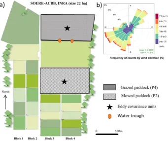
experimental set up of eddy covariance and a detailed footprint study was performed [26]. The wind rose, which is identical for the two paddocks, is reported in Figure1. Footprint analysis indicated that ~70% of the median percentage of the footprint was in the field, which is a similar fraction than that
found in other similar studies [26].
For the present study, two temporary sown grasslands paddocks, each of a size of ~3 ha and of rectangular shape, were equipped with two eddy covariance measurement systems and a meteorological station (Figure1). One of the paddocks was regularly mowed (P2), with harvested hay exported off-site to feed animals during periods of insufficient vegetation growth (mainly drought periods and during winter). Dairy cows regularly grazed the other paddock (P4), with all animal excreta directly returned to the paddock, except for the fraction that was deposited offsite during milking and during the daily transit times from the milking shed to the field. Both paddocks received regular applications of nitrogen fertilizer, with higher rates applied to the mowed than the grazed paddock (AppendixA).
For the two contrasting grassland systems studied here, the dates of mowing and grazing, the length of each grazing event, the animal stocking densities, and timing and amounts of N fertilizer applications varied in the different years. Details are given in AppendixA. Over the 5-year study period (2006–2010) the mowed paddock received 1290 kg N ha−1split into 17 fertilizer applications and was mowed 17 times with 3 cuts per year, except for the wetter than normal summer half-year 2007 (5 cuts). Over the same period, the grazed paddock received 590 kg N ha−1(not including N returned in dung and urine during grazing) over 14 applications and was grazed 37 times with grazing events spread, on average, over 5 consecutive days.
Agronomy 2019, 9, x FOR PEER REVIEW 4 of 32
treatments relevant for the present work are two of the 3 ha plots with pasture being either mowed or grazed. The towers footprints are crucial in experimental set up of eddy covariance and a detailed footprint study was performed [26]. The wind rose, which is identical for the two paddocks, is reported in Figure 1. Footprint analysis indicated that ~70% of the median percentage of the footprint was in the field, which is a similar fraction than that found in other similar studies [26].
For the present study, two temporary sown grasslands paddocks, each of a size of ~3 ha and of rectangular shape, were equipped with two eddy covariance measurement systems and a meteorological station (Figure 1). One of the paddocks was regularly mowed (P2), with harvested hay exported off-site to feed animals during periods of insufficient vegetation growth (mainly drought periods and during winter). Dairy cows regularly grazed the other paddock (P4), with all animal excreta directly returned to the paddock, except for the fraction that was deposited off site during milking and during the daily transit times from the milking shed to the field. Both paddocks received regular applications of nitrogen fertilizer, with higher rates applied to the mowed than the grazed paddock (Appendix A).
For the two contrasting grassland systems studied here, the dates of mowing and grazing, the length of each grazing event, the animal stocking densities, and timing and amounts of N fertilizer applications varied in the different years. Details are given in Appendix A. Over the 5-year study period (2006–2010) the mowed paddock received 1290 kg N ha−1 split into 17 fertilizer applications and was mowed 17 times with 3 cuts per year, except for the wetter than normal summer half-year 2007 (5 cuts). Over the same period, the grazed paddock received 590 kg N ha−1 (not including N returned in dung and urine during grazing) over 14 applications and was grazed 37 times with grazing events spread, on average, over 5 consecutive days.
Figure 1. (a) Field site layout of the Agroecosystem Biogeochemical Cycles and Biodiversity (ACBB) experimental farm (22 ha). Different colors are used to distinguish different treatments. The treatments relevant for the present work are shown by stars indicating the location of the eddy
2.1.1. Meteorological Conditions at the Study Site
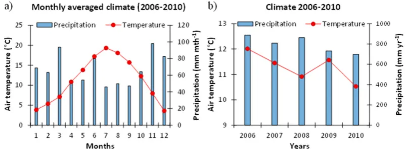
Meteorological conditions for the two paddocks were acquired from a weather station coupled to a data logger (CR-10X, Campbell Scientific Inc., Logan, UT) placed 1.9 meters aboveground on the mown paddock [17,26,61]. Briefly, the weather station provided 30 min averaged values of precipitation (SBS500, Campbell Scientific Inc., Logan, UT), air temperature and relative humidity (HMP 45 AC, Vaisala), radiation components (CNR1, Kipp & Zonen), and wind speed (A100L2, Vector Instruments) and direction (W200P, Vector Instruments). Volumetric soil water content data were collected by time domain reflectometry (TDR) probes at 10, 20, 30, 60, 80, and 100 cm depths (CS616, Campbell Scientific Inc., Logan, UT), and soil temperatures were measured at 5, 10, 20, 30, 60, 80, and 100 cm down the soil profile (PT100, Mesurex), but only for the mowed paddock. Soil heat flux was measured at 5-cm-depth (HFP01, Hukseflux), and data were corrected for changes in heat storage in the soil layer above the flux plate [62]. Over the study period (2006–2010), average air temperature and average annual precipitation were 11.2◦C and 774 mm yr−1, respectively. Half-hourly meteorological data, i.e., air temperature, global radiation, humidity, and precipitation, were summed/averaged to daily values to be used as driving variables for the CenW model runs of both paddocks.
The predominant wind direction was from the southwest and a secondary peak from the northeast (Figure1b).
Throughout the five years of the study, daily maximum air temperature exceeded 25◦C for 10.5% of the time, with a maximum of 35.5◦C. Daily minimum air temperature was negative for 13.3% of the time, with a lowest value of−11.0◦C (data not shown). Summer months (June–September) were hot
and dry with average monthly air temperature ranging between 15.6 and 19.4◦C and precipitations between 48 and 71 mm mth−1(Figure2a). The wettest and coldest month are November (98 mm mth−1) and December (3.6◦C), respectively (Figure2a). Among the five years of the study, 2006 was the warmest (11.9◦C) and wettest (888 mm yr−1), while 2010 was the coldest (10.5◦C) and driest (697 mm yr−1) year.
covariance masts on the two studied paddocks (P2: mowed paddock; P4: grazed paddock). (b) The
wind rose shows the frequency and intensity of winds blowing from different directions. The length of each "spoke" around the circle is related to the frequency of time that the wind blows from the specified direction.
2.1.1. Meteorological Conditions at the Study Site
Meteorological conditions for the two paddocks were acquired from a weather station coupled to a data logger (CR-10X, Campbell Scientific Inc., Logan, UT) placed 1.9 meters aboveground on the mown paddock [17,26,61]. Briefly, the weather station provided 30 min averaged values of precipitation (SBS500, Campbell Scientific Inc., Logan, UT), air temperature and relative humidity (HMP 45 AC, Vaisala), radiation components (CNR1, Kipp & Zonen), and wind speed (A100L2, Vector Instruments) and direction (W200P, Vector Instruments). Volumetric soil water content data were collected by time domain reflectometry (TDR) probes at 10, 20, 30, 60, 80, and 100 cm depths (CS616, Campbell Scientific Inc., Logan, UT), and soil temperatures were measured at 5, 10, 20, 30, 60, 80, and 100 cm down the soil profile (PT100, Mesurex), but only for the mowed paddock. Soil heat flux was measured at 5-cm-depth (HFP01, Hukseflux), and data were corrected for changes in heat storage in the soil layer above the flux plate [62]. Over the study period (2006–2010), average air temperature and average annual precipitation were 11.2 °C and 774 mm yr−1, respectively. Half-hourly meteorological data, i.e., air temperature, global radiation, humidity, and precipitation, were summed/averaged to daily values to be used as driving variables for the CenW model runs of both paddocks.
The predominant wind direction was from the southwest and a secondary peak from the northeast (Figure 1b).
Throughout the five years of the study, daily maximum air temperature exceeded 25 °C for 10.5% of the time, with a maximum of 35.5 °C. Daily minimum air temperature was negative for 13.3% of the time, with a lowest value of −11.0 °C (data not shown). Summer months (June–September) were hot and dry with average monthly air temperature ranging between 15.6 and 19.4 °C and precipitations between 48 and 71 mm mth−1 (Figure 2a). The wettest and coldest month are November (98 mm mth−1) and December (3.6 °C), respectively (Figure 2a). Among the five years of the study, 2006 was the warmest (11.9 °C) and wettest (888 mm yr−1), while 2010 was the coldest (10.5 °C) and driest (697 mm yr−1) year.
Figure 2. Temporal variation of mean daily air temperature and precipitation over the experimental
period (2006–2010) monthly (a) and annual (b) time scales in Lusignan, France.
2.1.2. Eddy Covariance (EC) Measurements and Processing
We used paired eddy covariance systems for the 2006–2010 period because it provided EC data measurements for both mowed (P2) and grazed (P4) paddocks. The two EC systems recorded raw data at 20 Hz, and EddyPro® software (LI-COR Inc.) was used for postprocessing and the calculation
at 30-minute intervals for fluxes of CO2, momentum, and sensible and latent heat. Each EC unit
Figure 2.Temporal variation of mean daily air temperature and precipitation over the experimental period (2006–2010) monthly (a) and annual (b) time scales in Lusignan, France.
2.1.2. Eddy Covariance (EC) Measurements and Processing
Agronomy2019,9, 183 6 of 31
through photosynthesis) and positive ones indicate that the system is a source of carbon (release of CO2through respiration).
Based on previous work using these EC datasets [17,26], flux measurements, and quality checks were done according to the CarboEurope-IP guidelines [63]. The flux footprint distribution and random uncertainty were analyzed. High-frequency loss corrections [18,64] were not considered in flux processing process [26]. The Webb–Pearman–Leuning (WPL) correction [65] was applied except for the self-heating of the IRGA because of the sensor orientation [66]. All years of flux measurements for the two EC towers were quality checked and filtered with a custom R program. The quality check led to the rejection of half-hourly flux observations based on nine criteria:
1. NEE values lower than−35 or higher than 25µmol m−2s−1
2. NEE values higher than 3.5µmol m−2s−1when PAR was above 400µmol m−2s−1 3. NEE values lower than−2µmol m−2s−1when PAR was below 25µmol m−2s−1 4. Rn>300 W m−2and LE<0 W m−2
5. If precipitation>0 mm 6. If u*<0.1 m s−1
7. λE values higher than 750 or lower than−100 W m−2
8. H values higher than 750 or lower than−100 W m−2
9. Atmospheric CO2concentration higher than 650 or lower than 320 ppm, respectively.
Common time series of eddy covariance measurements unavoidably include missing data due to power failures, instrumental malfunctions, or unfavorable micrometeorological conditions that cause the rejection of observations through the filtering process of data. However, complete time series of EC data at the half-hourly timescale are required to be summed to daily, monthly, or annual values [67,68]. Over the five years of EC measurements used in this study, there were gaps for 39.7% and 40.9% of NEE observations in the dataset for the mowed and grazed paddocks, respectively.
Gaps in 30 minutes NEE were filled and NEE was partitioned between GPP and total ecosystem respiration rate (ER) using the online gap-filling and flux partitioning procedure described by Reichstein et al. (2005) [69], hereafter referred to the Reichstein algorithm. This gap-filling method uses an improved, running-window look-up table that utilizes both the covariation of NEE with meteorological conditions and temporal autocorrelation of NEE [70]. In the Reichstein algorithm, ER was modeled using the Lloyd and Taylor equation [71] fitted to air temperature. Following this approach, nighttime ER was first regressed against nighttime air temperature, and this relationship was then used to estimate ER for both nighttime and daytime. GPP was determined by subtracting the parameterized ER from NEE.
2.1.3. Vegetation and Soil Organic Carbon Measurements
Harvested hay production (mowed paddock) was measured after each mowing event (TableA1). The total amount of harvested C was calculated by multiplying hay dry matter weight by the C concentration in biomass. Harvested biomass samples were collected from 6 replicates of 7.5 m2and oven dried at 60◦C. C concentration in the hay was measured in five replicates by dry combustion using a LECO C analyzer (TruSpecR CN Analyser; LECO Corporation, St Joseph, MI, USA).
Aboveground biomass present on the grazed paddock was measured just before and after each grazing event on six replicates within the field. Samples were oven dried and their C concentration measured with the same method than for harvested hay production.
Root biomass of the different treatments was measured once a year in three soil horizons (0–30, 30–60, and 60–90 cm). Each measurement is the average of twelve samples from a 6.5 cm∅
mechanical auger.
used to set up the water dynamic procedure of the CenW model and total soil organic carbon content measured in 2005 was use to initialize the model.
2.2. Modeling Details
2.2.1. CenW 4.2 Overview
CenW is an open-source process-based model, combining the major carbon, energy, nutrient, and water fluxes in an ecosystem [52]. For the present work, we used CenW version 4.2, which is available for download, together with its source code and a list of relevant equations available incenW
documentation, version 4.1.1 (A growth and C balance simulation model,©2017). A number of additional routines were added to run the model for managed pastures [56]. A list of relevant parameters is given in AppendixB. The CenW model runs on a daily time step and encompasses major ecosystem processes (canopy photosynthesis, allocation and growth, litterfall, decomposition, autotrophic and heterotrophic respiration), and their relationships to climatic drivers to simulate the behavior of the ecosystem over time, which are further modified through management practices (i.e., mowing, grazing, N fertilizer applications, plowing, and sowing).
The main CO2 fluxes are photosynthetic carbon gain by plants which is integrated over the whole canopy and the whole daytime period [72] and CO2losses through autotrophic respiration by plants and heterotrophic respiration by soil organisms and grazing animals, when they are present on the modeled paddock. CenW simulates soil heterotrophic respiration individually for growth and maintenance. These fluxes are modified by temperature and nutrient and water balances. Plant growth is determined by the dynamic allocation of fixed carbon to the different plant organs, which depends on the plant root/shoot ratio, vegetation type and development stages, and water and nutrient stresses. The model contains a fully integrated nitrogen cycle as well as a coupled multilayer bucket water model. Water is gained by rainfall and lost through evapotranspiration. Any amount of water exceeding the soil’s water-holding capacity is lost by deep drainage beyond the root zone, with important controls by soil depth and water-holding capacity. CenW simulates total evapotranspiration by modeling separately canopy and soil evaporation rates, and plant transpiration. These individual fluxes are calculated using the Penman–Monteith equation, with canopy resistance for calculating transpiration explicitly linked to photosynthetic carbon gain. This module of CenW is particularly important, as it is likely that soil water availability constituted an important constraint on plant productivity over the summer months at the experimental site, which is prone to summer droughts.
The soil organic matter component of CenW is based on the CENTURY model [55], which was originally developed for grasslands. The model includes three soil organic matter pools (active, slow, and resistant) with different potential decomposition rates. Leaves and roots senescence and litter production are controlled by plant type and phenology, and by water, temperature, and specific senescence parameters which depend on plant species. Dead foliage can either fall onto the soil surface and become part of the decomposing litter pool, remain standing for some time where it either decomposes during wet periods, or eventually falls onto the soil surface after some time. It was important to model these processes as the estimates of foliage biomass included a component of dead standing biomass that was not separated out in the data. These processes were modeled by assuming that all senescence, or drought-induced leaf death, initially transferred foliage from a live to a dead foliage pool [56]. The soil is divided into multiple layers and the same calculations driving the behavior of organic matter are applied to all of them, with each layer having its own complement of all organic matter pools. Layers only differ by the amounts and qualities of litter entering each layer. In addition, a small fraction of each pool is transferred to the corresponding pool in the layer below [53,73]. This allows changes in organic matter and C:N ratios in the surface litter layer and with depth in the soil to be simulated.
Agronomy2019,9, 183 8 of 31
“grazed” paddock of the Lusignan study farm described above, the model assumed (similar to the study of a dairy farm in New Zealand [56]) that cows consumed, at each grazing event, a given amount of above ground biomass [74]. If grazing was spread over several consecutive days, grazing percentages on individual days were adjusted to add to a total of that fixed percentage at the end of the grazing events. Of that feed, 50% was assumed to be lost by respiration [75], 5% as methane [76], and 18% removed as milk solids [15,75,77], with the remaining 27% returned to the paddock as dung and urine. It is also assumed that animal weights remained constant and not added to carbon gains or losses from the paddocks. For the mowed paddock it is assumed in the model that during each harvest event, a given amount (depending on total above ground biomass and cutting height) of aboveground photosynthesizing biomass is cut, and of that amount 95% is exported from the farm with the 5% remaining being left on the pasture as residues.
2.2.2. Model Parameterization and Statistical Analysis
Harvested hay production was measured after each mowing event for the mowed paddock and the amounts of biomass on the grazed paddock were measured just before and after each grazing events. These observations were used to constrain the grazing and harvesting procedures in CenW simulations and measured root biomass and soil water contents at different depth in the soil were used to constrain the soil water extraction of the CenW ecosystem model.
Total SOC content was measured in early 2005 for different soil layers and for the two managed grasslands (mowed and grazed), and these values were used to initialize the CenW model independently for the two paddocks through the spin up of the model simulations until equilibrium conditions between measured and modeled initial SOC stocks were reached.
Model simulations were optimized by selecting a set of parameter values that minimized the residual sums of squares across different EC measurements and ancillary observations. Measurements used for CenW parameterization were daily- and weekly-averaged estimates of evapotranspiration (ET) and net ecosystem exchange (NEE). We separated our five years of eddy covariance data into weekly sets, with one week of daily values used for parameter optimization and the other week for model validation. There are therefore two flux datasets for each paddock, one for model calibration, and one for model verification. CenW uses an automatic parameter optimization routine that worked by changing parameter values within specified boundaries to minimize the residual sums of squares. That was applied to both daily and weekly-averaged data within the data set selected for parameter optimization.
Initial parameter values to run CenW for managed grasslands were retrieved from a previous study where the model was run for a grazed dairy farm of New Zealand [56]. Specific management practices from farm records were implemented in CenW and we used a spin up of the model to initialize soil carbon and nitrogen pools. Then, model simulations were optimized for these paddocks based on a selection of eddy covariance observations (NEE and ET) and ancillary data (amounts of vegetation mowed and grazed and soil water content) by the automatic parameter optimization procedure imbedded in the model that aim to maximize the agreement between model and observations.
The overall goodness of fit was described by the Nash–Sutcliffe model efficiency (EF) [78]:
EF=1−
P
(yo−ym)2
P
(yo−y)2
, (1)
whereyorepresents the individual observations,ymis the corresponding modeled values, andythe
the model, while positive values indicate that the model is a better predictor than the observed mean. The closer EF is to one, the stronger the agreement between observed and modeled data.
The final sets of parameters values used for the simulations of the mown and grazed paddocks are given in AppendixB.
3. Results
3.1. CenW Performances to Simulate Carbon Dioxide and Water Fluxes of Mown and Grazed Grasslands
Over the five years of the study period, a wide range of climatic conditions (Figure2) were encountered as well as different management practices like different mowing, grazing, and fertilizer application frequencies (AppendixA) and different stocking rates for the various grazing events. Achieving good model/data agreement is challenging because the model needs to incorporate a wide variety of processes to simulate accurately such complex systems and to capture the variability of fluxes and vegetation dynamics affected by biotic and abiotic factors. The CenW model used only one fixed set of parameters for multiple years and after the calibration of the CenW model for the two grassland sites, daily modeled and observed carbon and water fluxes could be compared.
3.1.1. Carbon Dioxide Fluxes
Comparisons between modeled and measured daily CO2fluxes for the two differently managed grasslands are shown in Figure3, and model efficiencies for model calibration and validation are given in Table1. In this section, only the best quality data from background periods (outside mowing and grazing events) were used for the comparisons. Observations that would have been affected by mowing and grazing events were omitted from the analyses [56], as well as days when fluxes from the eddy covariance systems had to be gap filled for more than 1/3 of half hourly periods. This selection of only best quality observation was necessary to avoid
1. the calibration of the model with data that strongly depended on another simpler model (i.e., the Reichstein gap-filling and partitioning tool) and
2. to limit the bias that would have resulted from the non or incomplete capture by EC of the large respiratory losses during measurement periods when grazing animals were present around the EC tower or when freshly cut or drying grass was present on the ground during mowing events [56,79].
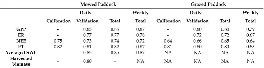
Table 1.Model efficiencies for six key observations of the two-modeled systems. Only daily NEE and ET were used for the model parameterization. ‘Total’ refers to the complete data set that included data in both the parameterization and validation data sets.
Mowed Paddock Grazed Paddock
Daily Weekly Daily Weekly
Calibration Validation Total Total Calibration Validation Total Total
GPP - 0.85 0.85 0.87 - 0.80 0.80 0.79
ER - 0.77 0.77 0.78 - 0.72 0.72 0.67
NEE 0.75 0.73 0.74 0.72 0.64 0.66 0.65 0.64
ET 0.82 0.81 0.82 0.87 0.81 0.80 0.80 0.85
Averaged SWC - 0.85 0.85 0.87 NA NA NA NA
Harvested
biomass - 0.80 - NA NA NA NA NA
Agronomy2019,9, 183 10 of 31
than the relatively small difference between the two (NEE). Model/data agreements are also better for mowing than for grazing, certainly because of the higher complexity of grazed systems compared to mowing. On the one hand, for the mowed paddock, management practices (mowing events and fertilizer applications) are accomplished within a day and evenly applied to the field. While, on the other hand, for the grazed paddock, grazing events last several consecutive days, the stocking density vary for the different events, there are dung and urine patches, there is an uneven reparation of cattle on the paddock, there could be some preferential grazing of plant species, and pasture could be damaged by trampling.Agronomy 2019, 9, x FOR PEER REVIEW 11 of 32
Figure 3. Scatter plots of observed vs. modeled daily carbon fluxes for the mown (panels a–c) and
grazed (panels d–f) paddocks, for background measurement periods outside management (grazing,
mowing) events. For NEE, negative numbers refer to carbon gain by the system. Corresponding model efficiencies for each comparison are given in Table 1.
3.1.2. Soil Water Content and Evapotranspiration
Evapotranspiration (ET) measurements were also used for the parameterization and validation of the CenW model for both grassland sites. Soil water content observations were only available for the mowed paddock and were not used for the calibration of the model. Figure 4 shows the time series of daily observed and modeled soil water content (SWC) of the mowed paddock for three depths averaged over the entire soil profile.
Over the entire study period, the soil water content measured and modeled at different depth agree quite well (Figure 4a–c), confirming the correct set up of the soil water flows procedure in CenW. Averaged soil water content was generally well modeled, with an EF of 0.83. On average, over the study period and over the entire soil profile, modeled and measured SWC were 22.4% and 21.9%, respectively.
After parameterizing the model with good quality data over the full length of the study period (2006–2010), we obtained good agreement between modeled and observed carbon fluxes. Figure3a,b shows the comparison of daily modeled GPP against their observation-based counterparts for the mowed and grazed paddocks, respectively. Good agreement was shown for both managed grasslands by the slopes close to 1, small intercepts of the linear regressions, and high correlation coefficients (R2=0.80–0.90). For the mowed paddock, model efficiencies for GPP were 0.86 and 0.88 for daily and weekly averaged fluxes, respectively (Table1). Slightly lower, but still good EF was also found for GPP of the grazed paddock with daily and weekly model efficiencies of 0.80 and 0.79, respectively (Table1).
The model also showed good performance in simulating daily and weekly averaged ecosystem respiration rates for both sites. For instance, the daily EF and R2were 0.79 and 0.85 for the mowed and 0.73 and 0.71 for the grazed paddocks, respectively (Figure3b,e). The grazed paddock had higher ER values than the mowed paddock and there was more scatter in the model/data comparison (Figure3b,e) according to the lower values of R2for daily and weekly comparisons.
The comparison of modeled NEE with EC measurements showed that the CenW model performed well in capturing the variability in NEE in background conditions. Across the two studied grassland sites, the CenW model explained between 65 and 74% of the variation in daily NEE for the mowed and grazed paddocks, respectively (Figure3c,f and Table1). For the mowed paddock, the coefficients of determination for daily and weekly averaged net carbon fluxes were 0.74 and 0.77, respectively (Table1). The agreement between observed and modeled NEE for the grazed paddock was lower than for the mown paddock with daily and weekly R2of 0.65 and 0.71, respectively. For the two managed grasslands, the overall seasonal and annual variations in NEE are reasonably well modeled and consistent agreement between modeled and measured NEE was achieved with daily model efficiencies of 0.74 and 0.65 for the mowed and grazed paddocks, respectively.
3.1.2. Soil Water Content and Evapotranspiration
Evapotranspiration (ET) measurements were also used for the parameterization and validation of the CenW model for both grassland sites. Soil water content observations were only available for the mowed paddock and were not used for the calibration of the model. Figure4shows the time series of daily observed and modeled soil water content (SWC) of the mowed paddock for three depths averaged over the entire soil profile.
Over the entire study period, the soil water content measured and modeled at different depth agree quite well (Figure4a–c), confirming the correct set up of the soil water flows procedure in CenW. Averaged soil water content was generally well modeled, with an EF of 0.83. On average, over the study period and over the entire soil profile, modeled and measured SWC were 22.4% and 21.9%, respectively.
There was no systematic over- or underestimates of soil water content. Lower modeled SWC were found in spring 2006 and during summers of 2008 and 2010 (Figure4) and were most likely due to higher CenW modeled water losses in spring and early summer than actual field conditions. Conversely, measured SWC was sometimes lower than modeled values. In 2007, observed soil water drawdown was faster than model simulation, but Figure 6d shows no discrepancies in ET, and so the problem seems to be linked to water drawdown. It could be that CenW extracted too much water from deeper layers and preserved it in the top layers. This situation was encountered following a water-limited period and could be due to cracks in the soil, causing preferential water flows not accounted for in the model or to the incomplete capture of vegetation dynamic in response to droughts.
Agronomy2019,9, 183 12 of 31
is consistent with the good results reported for the modeling of daily and weekly evapotranspiration rates (Figure5a and Table1).
Agronomy 2019, 9, x FOR PEER REVIEW 12 of 32
There was no systematic over- or underestimates of soil water content. Lower modeled SWC were found in spring 2006 and during summers of 2008 and 2010 (Figure 4) and were most likely due to higher CenW modeled water losses in spring and early summer than actual field conditions. Conversely, measured SWC was sometimes lower than modeled values. In 2007, observed soil water drawdown was faster than model simulation, but Figure 6d shows no discrepancies in ET, and so the problem seems to be linked to water drawdown. It could be that CenW extracted too much water from deeper layers and preserved it in the top layers. This situation was encountered following a water-limited period and could be due to cracks in the soil, causing preferential water flows not accounted for in the model or to the incomplete capture of vegetation dynamic in response to droughts.
Figure 4. Time series of daily-modeled (black line) and observed (red symbols) soil water content at (a) 10 cm, (b) 30 cm, (c) 90 cm belowground, and (d) averaged over the whole soil profile (0–100 cm) for the mowed grassland.
Overall agreement for SWC is good, and remaining discrepancies could be due to measurement errors like the heavy rainfall in 2006 either not measured correctly, or not all water infiltrating but running off. Others could be due to shortcomings of the model, like not having soil cracks represented, or because of some measurement uncertainties reducing the model/data agreement. Because SWC and ET are tightly linked, achieving to get a good agreement between observed and modeled soil moisture is consistent with the good results reported for the modeling of daily and weekly evapotranspiration rates (Figure 5a and Table 1).
Figure 4.Time series of daily-modeled (black line) and observed (red symbols) soil water content at (a) 10 cm, (b) 30 cm, (c) 90 cm belowground, and (d) averaged over the whole soil profile (0–100 cm) for
the mowed grassland.Agronomy 2019, 9, x FOR PEER REVIEW 13 of 32
Figure 5. Scatter plots of observed vs. modeled evapotranspiration rates for the mown (a) and grazed
(b) paddocks.
The CenW model explained more than 80% of the variation in daily ET for the two grassland sites. There was a close agreement between modeled and observed daily ET across the monitoring period (Figure 5), with R2 of 0.82 and 0.81 and EF of 0.82 and 0.80 for mowed and grazed paddocks, respectively. The coefficients of the linear regression lines (Figure 5) show a tendency of the model to slightly underestimate low ET (positive intercepts) and overestimate high evapotranspiration rates (slopes lower than 1), however slopes and intercepts are very close to their optimal values, showing that there is no systematic differences between modeled and observed evapotranspiration rates.
Overall, very good agreements between the CenW modeled and observed daily CO2 and water
fluxes were achieved for both management practices (i.e., mowing and grazing). This indicated that the response of the model to climatic conditions and management practices were well captured in the simulations and that most of the processes encountered in the fields were properly implemented
in CenW. Student’s t-tests were used to statistically test if slopes of linear regressions were
significantly different from 1 and intercepts different than 0. Results showed that for water and all carbon fluxes, except NEE, for the two grasslands management, the slopes and intercepts were significant (p-values < 0.05). Even though GPP and ER were not used to parameterize CenW, there was nonetheless very good agreement between simulations and measurements (Figure 3a–d and Table 1). This indicate a high correlation between photosynthesis and ecosystem respiration rates derived from NEE data according to the Reichstein partitioning algorithm and fluxes modeled by the mechanistic CenW model.
3.2. Seasonal and Interannual Variabilities of Modeled and Observed Carbon Dioxide and Water Fluxes
3.2.1. Day-to-Day and Seasonal CO2 and Water Fluxes Variability
For managed grassland ecosystems, important drivers of day-to-day and seasonal variabilities are management practices, particularly the timing and intensity of mowing and grazing that combine with the natural temporal climate variability to drive the behavior of ecosystems and strongly affect the CO2 dynamic and C balance of managed grasslands [8].
Depending on a number of climatic factors (solar radiation, temperature, and precipitation), ecological factors (leaf area and water, nutrient, and temperature stresses), and management practices (nitrogen fertilization, mowing and grazing timing, duration, and intensity), modeled and observed CO2 and water fluxes demonstrate pronounced temporal dynamics over several years [79], as exemplified by the time series presented in Figures 6 and 7.
The apparent day-to-day and seasonal variabilities of observation based GPP was well captured by the CenW model for both of the managed grassland sites (Figures 6a and 7a). The highest assimilation rates occurred during spring and summer, with GPP values up to 160 kgC ha−1 d−1 when growth conditions were the most favorable. Over the summer months, both modeled and observed GPP were reduced through water limitations, which occurred over most summer months but varied in intensity from year to year. Lower CO2 assimilations rates were found during the winter months
Figure 5.Scatter plots of observed vs. modeled evapotranspiration rates for the mown (a) and grazed (b) paddocks.
The CenW model explained more than 80% of the variation in daily ET for the two grassland sites. There was a close agreement between modeled and observed daily ET across the monitoring period (Figure5), with R2of 0.82 and 0.81 and EF of 0.82 and 0.80 for mowed and grazed paddocks, respectively. The coefficients of the linear regression lines (Figure5) show a tendency of the model to slightly underestimate low ET (positive intercepts) and overestimate high evapotranspiration rates (slopes lower than 1), however slopes and intercepts are very close to their optimal values, showing that there is no systematic differences between modeled and observed evapotranspiration rates.
CenW. Student’st-tests were used to statistically test if slopes of linear regressions were significantly different from 1 and intercepts different than 0. Results showed that for water and all carbon fluxes, except NEE, for the two grasslands management, the slopes and intercepts were significant (p-values< 0.05). Even though GPP and ER were not used to parameterize CenW, there was nonetheless very good agreement between simulations and measurements (Figure3a–d and Table1). This indicate a high correlation between photosynthesis and ecosystem respiration rates derived from NEE data according to the Reichstein partitioning algorithm and fluxes modeled by the mechanistic CenW model.
3.2. Seasonal and Interannual Variabilities of Modeled and Observed Carbon Dioxide and Water Fluxes
3.2.1. Day-to-Day and Seasonal CO2and Water Fluxes Variability
For managed grassland ecosystems, important drivers of day-to-day and seasonal variabilities are management practices, particularly the timing and intensity of mowing and grazing that combine with the natural temporal climate variability to drive the behavior of ecosystems and strongly affect the CO2dynamic and C balance of managed grasslands [8].
Depending on a number of climatic factors (solar radiation, temperature, and precipitation), ecological factors (leaf area and water, nutrient, and temperature stresses), and management practices (nitrogen fertilization, mowing and grazing timing, duration, and intensity), modeled and observed CO2 and water fluxes demonstrate pronounced temporal dynamics over several years [79], as exemplified by the time series presented in Figures6and7.
The apparent day-to-day and seasonal variabilities of observation based GPP was well captured by the CenW model for both of the managed grassland sites (Figures6a and7a). The highest assimilation rates occurred during spring and summer, with GPP values up to 160 kgC ha−1
d−1
when growth conditions were the most favorable. Over the summer months, both modeled and observed GPP were reduced through water limitations, which occurred over most summer months but varied in intensity from year to year. Lower CO2assimilations rates were found during the winter months as temperature and radiation were low and limited photosynthesis and vegetation growth, but some gas exchange continued throughout even the coldest winters. After mowing events, during the peak growing season, GPP was strongly reduced down to wintertime levels. GPP typically dropped from preharvest values in the range of 120 to 160 kgC ha−1d−1to postharvest values between 20 and 50 kg C ha−1d−1(Figures 6a and7a). These reductions of GPP by 2/3 are important and even if, on average, only three harvests were carried out each year, they have significant and long-lasting effects on ecosystem behavior and gas exchange. CenW managed to simulate accurately the recovery of the ecosystem gas exchanges rates (Figure6, Figure7, and FigureA1) after cutting and grazing events.
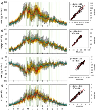
The day-to-day variability of observation-derived ER was also reasonably well captured in the model simulation and the seasonal pattern was well reproduced, in particular, displaying ongoing reasonably high respiration rates throughout the winter months (Figure6b). Harvesting did not affect ER as strongly as GPP (Figure6a,b) since autotrophic respiration from above ground vegetation is only part of the total ecosystem respiration, and (belowground) heterotrophic respiration was mostly unaffected by harvests. Because NEE is the difference between the two large fluxes of C assimilation through photosynthesis (GPP) and ecosystem respiration (ER), it was also affected by vegetation harvests (Figure6c).
Agronomy2019,9, 183 14 of 31
Agronomy 2019, 9, x FOR PEER REVIEW 14 of 32
as temperature and radiation were low and limited photosynthesis and vegetation growth, but some gas exchange continued throughout even the coldest winters. After mowing events, during the peak growing season, GPP was strongly reduced down to wintertime levels. GPP typically dropped from
preharvest values in the range of 120 to 160 kgC ha−1 d−1 to postharvest values between 20 and 50 kg
C ha−1 d−1 (Figures 6a and 7a). These reductions of GPP by 2/3 are important and even if, on average,
only three harvests were carried out each year, they have significant and long-lasting effects on ecosystem behavior and gas exchange. CenW managed to simulate accurately the recovery of the ecosystem gas exchanges rates (Figures 6,7, and C1) after cutting and grazing events.
The day-to-day variability of observation-derived ER was also reasonably well captured in the model simulation and the seasonal pattern was well reproduced, in particular, displaying ongoing reasonably high respiration rates throughout the winter months (Figure 6b). Harvesting did not affect ER as strongly as GPP (Figure 6a,b) since autotrophic respiration from above ground vegetation is only part of the total ecosystem respiration, and (belowground) heterotrophic respiration was mostly unaffected by harvests. Because NEE is the difference between the two large fluxes of C assimilation through photosynthesis (GPP) and ecosystem respiration (ER), it was also affected by vegetation harvests (Figure 6c).
Figure 6. Time series of modeled (black line) and observed (red dots) daily carbon fluxes (a) GPP, (b) ER, and (c) NEE, and water fluxes (d) ET for the mowed grassland site. Vertical green lines represent mowing events.
Figure 6.Time series of modeled (black line) and observed (red dots) daily carbon fluxes (a) GPP, (b) ER, and (c) NEE, and water fluxes (d) ET for the mowed grassland site. Vertical green lines represent mowing events.
Evapotranspiration flux (ET) was highest during spring and summer when climatic conditions were the most favorable for water losses and vegetation was the most active (Figure6d). The removal of aboveground biomass by harvesting or grazing led to sharp reductions of the transpiration rates, partially compensated by the increase in soil transpiration caused by an increase of solar radiation reaching—and higher temperature at—the soil surface.
Grazing events greatly affected GPP and ET (Figure7a,d) and caused massive spikes in modeled ER due to cattle respiration (Figure7b). Similarly to the mowed paddock discussed above, the removal of photosynthesizing biomass by grazing animal caused an important subsequent reduction in carbon assimilation rates (GPP). However, in contrast to harvest events which were sudden and restricted to single days, the removal of biomass by dairy cows was progressive and spread over several consecutive days (on average five days). GPP reductions were therefore not as abrupt as for the mowed grassland (Figures6a,7a andA1) and generally, postgrazing daily modeled and observed GPP values agreed well and remained higher than postharvest values, which most likely resulted from the extent of biomass removal that differ between the two treatments.
CenW simulations, the grazing animal respiration rate is 4.15 kg C head−1d−1(4µmol CO2head−1 s−1). In some cases, such pulses were visible but much smaller in the eddy covariance measurements than in the model. Measurements could only record what happened within the flux footprint, which varied with wind speed and direction while the CenW model simulated the whole paddock. If all dairy cows were not inside the footprint at any given time, it would have been impossible for the EC tower to measure total grazing animals’ respiration while it was fully accounted for in the CenW model. At other times, a large number of cows might have been present within the flux footprint and their respiration would have been captured by the EC system. However, because this rate could have been an order of magnitude higher than the base respiratory carbon flux from the soil and pasture [56] the corresponding data could have been filtered out during the processing of EC fluxes. If the resultant data gaps during grazing events were filled using the traditional Reichstein gap-filling and partitioning algorithms it could have resulted in gaps being filled based on data collected during periods in the preceding and following week when there were no cows present within the flux footprint.
Agronomy 2019, 9, x FOR PEER REVIEW 16 of 32
Figure 7. Time series of modeled (black line) and observed (red dots) daily carbon fluxes and water fluxes (a) GPP, (b) ER, (c) NEE, and (d) ET for the grazed grassland site. Vertical green lines represent grazing events.
3.2.2. Interannual Variability of CenW Modeled and EC Measurements of CO2 and H2O Fluxes
Interannual Variations in Mean Daily Fluxes
Generally, daily modeled and observed fluxes averaged over the five years of the study agreed very well for the mowed grassland site, as well as their interannual variations (+/– 1 SE from the 5-year daily averages). This is highlighted in Figure 8 by error bars (for EC observed fluxes) and yellow area (for CenW modeled fluxes) and confirms that the CenW model simulations captured well the fluxes variations due to differences in meteorological conditions and management for the mowed paddock.
Higher interannual variability was found during the most productive seasons (spring and summer), in which most of the harvest events occurred (on different days each year). GPP is more variable than ER because of the larger direct impact of harvest on photosynthesizing biomass that on total ER. Water limiting conditions and the onset of harvest events (end of April–early May) led to a
Agronomy2019,9, 183 16 of 31
3.2.2. Interannual Variability of CenW Modeled and EC Measurements of CO2and H2O Fluxes
Interannual Variations in Mean Daily Fluxes
Generally, daily modeled and observed fluxes averaged over the five years of the study agreed very well for the mowed grassland site, as well as their interannual variations (+/– 1 SE from the 5-year daily averages). This is highlighted in Figure8by error bars (for EC observed fluxes) and yellow area (for CenW modeled fluxes) and confirms that the CenW model simulations captured well the fluxes variations due to differences in meteorological conditions and management for the mowed paddock.
Agronomy 2019, 9, x FOR PEER REVIEW 17 of 32
substantial reduction of GPP and hence of the net ecosystem exchange rate with NEE averaged values during this period as low as wintertime fluxes.
Figure 8. Daily carbon and water fluxes averaged for each day of the year over the study period (2006–2010) for the mowed pasture. The blue circles are used for observations, error bars represent one standard deviation around observed means; the red line is used for CenW modeled fluxes; and the yellow shaded areas represent one standard deviation around modeled means. GPP (a), ER (b), NEE (c), and ET (d).
For the grazed paddock, modeled and observed daily averages (over five years) agree very well for GPP (Figure 9a), as well as their interannual variability (error bars), confirming that the main biotic and abiotic factors controlling the dynamic of GPP were properly incorporated in the CenW ecosystem model. Weaker correlations were found between observed and modeled ER (Figure 9b) and NEE (Figure 9c) during grazing events while outside of grazing periods good agreements were retrieved. These large differences were likely caused by the noncapture of some or all of grazing animals’ respiration by the EC system.
Figure 8. Daily carbon and water fluxes averaged for each day of the year over the study period (2006–2010) for the mowed pasture. The blue circles are used for observations, error bars represent one standard deviation around observed means; the red line is used for CenW modeled fluxes; and the yellow shaded areas represent one standard deviation around modeled means. GPP (a), ER (b), NEE (c), and ET (d).
For the grazed paddock, modeled and observed daily averages (over five years) agree very well for GPP (Figure9a), as well as their interannual variability (error bars), confirming that the main biotic and abiotic factors controlling the dynamic of GPP were properly incorporated in the CenW ecosystem model. Weaker correlations were found between observed and modeled ER (Figure9b) and NEE (Figure9c) during grazing events while outside of grazing periods good agreements were retrieved. These large differences were likely caused by the noncapture of some or all of grazing animals’ respiration by the EC system.
Agronomy 2019, 9, x FOR PEER REVIEW 18 of 32
Figure 9. Daily carbon and water fluxes averaged for each day of the year over the study period (2006–2010) for the grazed pasture. Blue circles are used for observations, error bars represent one standard deviation around observed means; the red line is used for CenW modeled fluxes; and the
yellow shaded areas represent one standard deviation around modeled means. GPP (a), ER (b), NEE
(c), and ET (d).
Overall, model/data agreements are greatly variable and strongly depend of climate conditions and management practices (Figures 8 and 9).
Variability of Annual CO2 and Water Fluxes
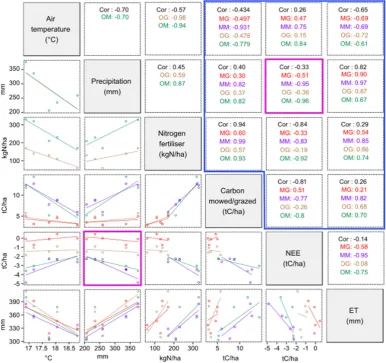
Correlations between climate, management practices and CO2 and water fluxes are showed
through a matrix plot (Figure 10). The different categories correspond to modeled and observed variables for the mowed and grazed paddocks. All points represent one year of either modeled or observed variables for the two sites summed/averaged over the summer half-year (15 April to 15 September), corresponding to the most productive time of the year. Lower panels show the scatter plots between the different selected variables and the upper panels give their correlation coefficients. For example, the pink-circled lower panel show the scatter plot of NEE and precipitation and the pink-circled upper panel give the corresponding correlation coefficients for the different categories
Figure 9. Daily carbon and water fluxes averaged for each day of the year over the study period (2006–2010) for the grazed pasture. Blue circles are used for observations, error bars represent one standard deviation around observed means; the red line is used for CenW modeled fluxes; and the yellow shaded areas represent one standard deviation around modeled means. GPP (a), ER (b), NEE (c), and ET (d).
Overall, model/data agreements are greatly variable and strongly depend of climate conditions and management practices (Figures8and9).
Variability of Annual CO2and Water Fluxes
Agronomy2019,9, 183 18 of 31
observed variables for the two sites summed/averaged over the summer half-year (15 April to 15 September), corresponding to the most productive time of the year. Lower panels show the scatter plots between the different selected variables and the upper panels give their correlation coefficients. For example, the pink-circled lower panel show the scatter plot of NEE and precipitation and the pink-circled upper panel give the corresponding correlation coefficients for the different categories (MG, MM, OG, and OM) and the overall correlation coefficient (Cor). The blue-circled area of the graph shows the selection of the most important relationships.
Agronomy 2019, 9, x FOR PEER REVIEW 19 of 32
(MG, MM, OG, and OM) and the overall correlation coefficient (Cor). The blue-circled area of the graph shows the selection of the most important relationships.
First, it is striking (Figure 10) that annual CO2 and H2O fluxes were correlated with annual meteorological condition (air temperature and precipitation) and with management practices (C harvested/grazed and N fertilizer applications) but with marked differences across the two managed grassland sites.
Figure 10. Matrix of paired plots showing the interannual variability of summer half-year (15th April–15th September) averaged climate drivers (air temperature and precipitation), management
practices (N fertilizer application and amounts of C mowed/grazed), and observed and modeled CO2
and H2O fluxes for the mowed and grazed grassland sites (MG: modeled grazing; MM: modeled
mowing; OG: observed grazing; OM: observed mowing). Variable names are given in the matrix diagonal. Paired scatterplots are in the lower triangle (below the diagonal in gray) with every point being the summer half-year of one year of the study period and colors are related to the different categories listed above. Their corresponding Pearson (linear) correlation coefficients are listed in the upper triangle (above the diagonal in gray). For example, the relationships between NEE and precipitation is shown in the pink circled scatter plot below the matrix diagonal and corresponding correlation coefficients for the different categories are given in the symmetric panel above the matrix diagonal (pink-circled). Important relationships are circled in blue on the upper panels.
For the mowed paddock, observed, and modeled amounts of carbon harvested are highly correlated with air temperature (OM: −0.78 and MM: −0.93), precipitation (OM and MM: 0.82), and N
Figure 10. Matrix of paired plots showing the interannual variability of summer half-year (15th April–15th September) averaged climate drivers (air temperature and precipitation), management practices (N fertilizer application and amounts of C mowed/grazed), and observed and modeled CO2
and H2O fluxes for the mowed and grazed grassland sites (MG: modeled grazing; MM: modeled
mowing; OG: observed grazing; OM: observed mowing). Variable names are given in the matrix diagonal. Paired scatterplots are in the lower triangle (below the diagonal in gray) with every point being the summer half-year of one year of the study period and colors are related to the different categories listed above. Their corresponding Pearson (linear) correlation coefficients are listed in the upper triangle (above the diagonal in gray). For example, the relationships between NEE and precipitation is shown in the pink circled scatter plot below the matrix diagonal and corresponding correlation coefficients for the different categories are given in the symmetric panel above the matrix diagonal (pink-circled). Important relationships are circled in blue on the upper panels.
harvested/grazed and N fertilizer applications) but with marked differences across the two managed grassland sites.
For the mowed paddock, observed, and modeled amounts of carbon harvested are highly correlated with air temperature (OM:−0.78 and MM:−0.93), precipitation (OM and MM: 0.82), and N
fertilizer (OM: 0.93 and MM: 0.99). On the contrary, correlations for the grazed paddock were lowest with N fertilizer (OG: 0.57 and MG: 0.60) and weak with climate (|OG|and|MG| <0.50).
The analysis also showed that, for the mowed paddock, the modeled and observed NEE were highly correlated with climate and management practices, but that for the grazed paddock NEE values were only weekly correlated with other variables. In this section and like for all this study, negative NEE represent a net gain, and a positive NEE is a net loss of CO2for the ecosystem. It is interesting that for the grazed paddock, modeled, and observed summer half-year NEE responded differently to the amount of vegetation grazed (i.e., CenW giving a positive moderate correlation of NEE with the amount of vegetation grazed while observations were giving a week negative correlation). This is due to the differences between modeled and observation-derived ER rates during grazing events and CenW simulating higher ER rates during grazing events: the more vegetation is eaten the more NEE increased (reduction of the sink strength of the pasture).
There were also high correlations between ET, climate and management practices for both grasslands, with a general upward trend of ET as precipitation, amounts of N fertilizer and C mowed/grazed increased and a downward trend with the increase of air temperature. More water vapor is returned to the atmosphere when there was more rainfall compared to dryer and hotter spring and summer periods.
The modeled and observed annual (full year average/sum) carbon and water balances for the mowed and grazed paddocks are shown in Figure11. For the mowed paddock, observed annual GPP values ranged between 16 and 20.5 tC ha−1yr−1(five-year average: 18.2 tC ha−1yr−1) and modeled GPP values ranged between 15.3 and 22.7 tC ha−1yr−1
(five-year average: 19.2 tC ha−1yr−1
). For the grazed paddock, observed annual GPP values ranged between 15.9 and 20.3 tC ha−1yr−1(five-year average: 18.1 tC ha−1yr−1) and modeled GPP values ranged between 14.9 and 20.2 tC ha−1yr−1 (five-year average: 18.2 tC ha−1yr−1).
fertilizer (OM: 0.93 and MM: 0.99). On the contrary, correlations for the grazed paddock were lowest with N fertilizer (OG: 0.57 and MG: 0.60) and weak with climate (|OG| and |MG| <0.50).
The analysis also showed that, for the mowed paddock, the modeled and observed NEE were highly correlated with climate and management practices, but that for the grazed paddock NEE values were only weekly correlated with other variables. In this section and like for all this study, negative NEE represent a net gain, and a positive NEE is a net loss of CO2 for the ecosystem. It is
interesting that for the grazed paddock, modeled, and observed summer half-year NEE responded differently to the amount of vegetation grazed (i.e., CenW giving a positive moderate correlation of NEE with the amount of vegetation grazed while observations were giving a week negative correlation). This is due to the differences between modeled and observation-derived ER rates during grazing events and CenW simulating higher ER rates during grazing events: the more vegetation is eaten the more NEE increased (reduction of the sink strength of the pasture).
There were also high correlations between ET, climate and management practices for both grasslands, with a general upward trend of ET as precipitation, amounts of N fertilizer and C mowed/grazed increased and a downward trend with the increase of air temperature. More water vapor is returned to the atmosphere when there was more rainfall compared to dryer and hotter spring and summer periods.
The modeled and observed annual (full year average/sum) carbon and water balances for the mowed and grazed paddocks are shown in Figure 11. For the mowed paddock, observed annual GPP values ranged between 16 and 20.5 tC ha−1 yr−1 (five-year average: 18.2 tC ha−1 yr−1) and modeled
GPP values ranged between 15.3 and 22.7 tC ha−1 yr−1 (five-year average: 19.2 tC ha−1 yr−1). For the
grazed paddock, observed annual GPP values ranged between 15.9 and 20.3 tC ha−1 yr−1 (five-year
average: 18.1 tC ha−1 yr−1) and modeled GPP values ranged between 14.9 and 20.2 tC ha−1 yr−1
(five-year average: 18.2 tC ha−1 yr−1).
On all years but 2006, CenW-modeled ER for the mowed paddock were lower than annual sums of EC-derived ER (Figure 11) with annual modeled ER values between 12.7 and 16.1 tC ha−1
yr−1 (five-year average: 14.9 tC ha−1 yr−1), while observation-based ER values varied from 11.6 to 15.7
tC ha−1 yr−1 (five-year average: 14.1 tC ha−1 yr−1). For the grazed paddock, model/data differences
were even more important with annual EC-derived and modeled ER varying from 14.3 to 19.0 tC ha−1 yr−1 (five-year average: 16.3 tC ha−1 yr−1) and from 15.2 to 19.9 tC ha−1 yr−1 (five-year average: 18.3
tC ha−1 yr−1), respectively.
Figure 11. Bar plot showing modeled and observed annual CO2 and water balances for the mowed ((a)
and (c)) and grazed ((b) and (d)) paddocks. Carbon fluxes (NEE, GPP, ER, and C harvested are given in tC
ha−1 and precipitation and ET are given in mm yr−1).
Figure 11.Bar plot showing modeled and observed annual CO2and water balances for the mowed ((a)