Full matrix capture with time-efficient auto-focusing of unknown geometry through dual-layered media

FMC

This paper presents a method for time-efficient

auto-focusing through a profile of unknown geometry applicable

to immersion testing. It is demonstrated that capture of the

complete time domain signal using the full matrix capture

technique allows for rapid ultrasonic profile mapping of a

complex geometry through the use of Fermat’s principle to

find the point of incidence at the reflective interface. Through

advanced optimisation and parallelisation of the algorithms

over the graphic processing unit, it is demonstrated that

rapid inspections are possible, given that the geometry falls

within the limits defined for the algorithm. To demonstrate

this, a linear array transducer is mounted to a perspex shoe

where auto-focusing is performed to generate ultrasonic

imagery of side-drilled holes through a curved surface.

post-processing, CUDA, full matrix capture, digital signal processing.

1. Introduction

Ultrasonic array imaging is a useful inspection technique for the identification and classification of defects within solid structures and is now routinely used within a wide range of site and lab-based applications[1]_{. However, imaging a profile of complex} geometry coupling to a rigid linear array transducer can prove problematic (where direct contact is not always possible). Often, this is overcome by coupling through an intermediate medium such as a perspex shoe or a fluid, as in the case of immersion testing. The computational complexity involved in imaging through a dual media makes real-time inspection difficult, as variations in geometry directly influence the imaging algorithms.

Since the introduction of advanced ultrasonic data acquisition and imaging techniques such as full matrix capture (FMC) and the total focusing method (TFM)[2]_{, imaging through a non-planar} surface is a time-intensive task, where it is necessary to calculate the time of flight from each transmit/receive element combination to a given pixel in the region of interest through the refractive boundary. While extensive investigation has been undertaken in the efficient imaging of such data[3] _{it is often applied during} post-processing, some time after the inspection has been undertaken and where time-efficient processing is not a requirement. This is due in part to the much larger datasets associated with FMC, but also to the number of calculations required to effectively image ultrasonic data for a complex geometry.

In this paper, a method is described that allows for the real-time inspection of FMC-acquired data through a complex surface

that is applicable to immersion testing. Auto-focusing through the geometry was accomplished by mapping the surface using ultrasonic signal processing techniques, combined with an advanced software optimisation technique developed to run over the graphics processing unit for additional computational efficiency. This was tested experimentally and shown to have the benefit of allowing for the rapid post-processing of data with high frame rates and a low implementation cost.

2. Theoretical background

FMC is a data acquisition process that allows for the collection of the full time domain signal for every possible transmit/ receive combination of an array transducer[2]_{. With each element} transmitting sequentially, acquisition of the amplitude data is received over the whole array, producing a data size of n2 _(where

n is the number of elements in the array). Fully focused imaging

of this data is generated through a standard sum and beamforming approach based on the principles of the synthetic aperture focusing technique (SAFT) and referred to by several names[2,4]_{, dependent} on the purpose and field for which the algorithm was developed. For the purpose of this paper, this algorithm will be referred to as TFM[2]_.

For a standard one-dimensional linear array transducer the TFM algorithm is expressed in Equation (1), where a grid of pixel intensity values (I) are defined by dimensions x, z, for which time-of-flight calculations are performed for each transmit (tx) and receive (rx) combination. A Hilbert transform (h)[5] _{is applied to} convert the real-time domain signal into complex form, allowing the signal envelope to be found. Here, c represents the velocity of the material and xtx and xrx are the lateral positions of the transmitting

and receiving elements:

I x,z

( )

(

)

2

+z2₊

(

)

c

⎛

⎝ ⎜ ⎜

⎞

⎠ ⎟ ⎟

∑

2.2 Snell’s Law and Fermat’s principle

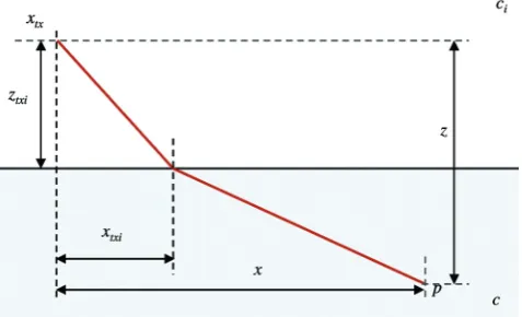
The direction of a beam at an interface point between two media of acoustic velocities ci and c can be calculated using the well-known Snell’s Law (as used for angle beam inspection to determine the path ultrasonic energy will take as it leaves the transducer and propagates through the refractive interface into the second medium). It can be shown that Snell’s Law is derived from Fermat’s principle of least time[6] _{as expressed here in Figure 1 and Equation} (2), where xtx, ztxi is the location of the point source and x, z is the

location P within the material. The point of incidence is determined as the location along the refractive interface which yields the minimum travel time. For a planar boundary, this point of interface may be calculated exactly using Snell’s Law as this yields a quartic polynomial to be solved analytically[7]_{. However, for a non-planar} surface it is necessary to explore an approximation to the solution through an iterative approach, where Fermat’s principle is applied

Full matrix capture with time-efficient auto-focusing of

unknown geometry through dual-layered media

M Sutcliffe, M Weston, P Charlton, K Donne, B Wright and I Cooper Submitted 03.10.12 Accepted 04.04.13

Mark Sutcliffe, Peter Charlton and Kelvin Donne are with Swansea Metropolitan University, Mt Pleasant Campus, Mt Pleasant, Swansea SA1 6ED, UK.

Mark Sutcliffe, Miles Weston, Ben Wright and Ian Cooper are with TWI NDT Validation Centre (Wales), ECM2_{, Heol Cefn Gwrgan, Margam, Port}

to sample points along the interface until a high enough degree of accuracy is determined:

time= xtxi2 +ztxi2

ci +

x−xtxi

(

)

+

(

)

c ...(2)

2.3 Focusing through dual media

Expanding Equation (1) to account for focusing through a refractive interface leads to Equation (3), where I is the intensity value for pixel location x, z, which is determined from the time-of-flight calculations for each tx, rx pair to the pixel region of interest via the point at which the ultrasonic energy passes through the refractive interface (xtxi, ztxi for transmit and xrxi, zrxi for receive). The velocity

in the medium is c and the velocity through the interface material is ci:

I x,z

( )

htx,rx

xtx−xtxi

(

)

txi2+

(

)

ci

+

(

)

(

)

(

)

(

)

c

⎛

⎝ ⎜ ⎜ ⎜ ⎜ ⎜

⎞

⎠ ⎟ ⎟ ⎟ ⎟ ⎟

∑

Calculation of xtxi, ztxi and xrxi, zrxi is determined iteratively

from Fermat’s principle of least time of flight and introduces an additional level of computational complexity impacting on the rate at which an inspection can occur.

3. Optimisation process

The principle of the focusing algorithm expressed in Equation (3) may be implemented with low memory requirements by looping through each x, z pixel location and then performing the necessary time-of-flight calculation for every transmit/receive (tx, rx) combination, thus requiring x × y ×

tx × rx calculations. As these calculations

involve trigonometric functions this approach is computationally expensive, and for time critical scenarios optimisations must be exploited.

For the use of FMC data, the application of a look-up table has been shown to provide a significant performance increase by reducing the number of calculations in favour of data retrieval operations[8]_{, but only at the} cost of increased memory requirements. For modern 64-bit computers this is less of an

issue as much more memory is addressable by an application than may previously have been available. For a planar surface, it can be observed that these calculations need only be performed once with relative values selected during the data processing stage. This would require a look-up table of dimensions x, z, tx, rx providing the storage requirements for the necessary performance boost. There would still remain an initial greater computationally expensive task as this look-up table is first populated, but for all subsequent operations retrieval of this pre-calculated data has been shown to be far quicker than without[8]_{; a technique that would work well for} inspections normal to the surface or where a fixed perspex shoe is used (as in the case of angle wedge inspection).

However, in the case of a non-planar surface of arbitrary geometry, there is a clear dependency on data and focal requirements prohibiting this approach (the focal requirements alter, dependent on where the transducer is positioned). Analysis of the algorithm reveals a repetition of calculations, allowing for reduced complexity if the use of a second look-up table is exploited. The inner loops of

tx and rx have an execution time of tx × rx, which can be reduced

to tx if calculations of the times of flight were performed on only the transmit portion of the formula with respect to every x, z. The

rx component can easily be obtained from two look-ups and an

addition operation by assuming the tx component relative to (x, z) is identical to the rx component relative to the (x, z) pixel location. For example, consider a 32-element linear array focusing on a region 100 × 100 pixels. In non-optimised form, 100 × 100 × 32 × 32 or 1024E4 time-of-flight calculations are required. Calculating only the tx components allows for a reduction to 100 × 100 × 32 or 32E4, where the correct time of flight is retrieved through the summation of look-up values (x, y, rx) + (x, y, tx). While this approach leads to an increased number of data retrieval operations, it is far more computationally efficient than performing each calculation in isolation. This relationship is illustrated in Figure 2, where it is shown that a look-up table of dimension x, z (tx × rx) is populated from a smaller look-up table of dimension x, z, tx. 3.1 The graphics processing unit

CUDA is a parallel programming model first introduced in 2006 by NVIDIA to allow for complex computational problems to execute over its architecture. Built around a scalable array of multithreaded streaming multiprocessors that are designed to execute hundreds of threads concurrently, thread management is controlled by the single instruction – multiple thread (SIMT) architecture made popular by the super computers of the 1970s[9]_{. Being unsuitable for} general-purpose computing, it has evolved to facilitate the rendering of 3D graphics where there is no dependency between threads[10]_.

Implemented as a subset of the C programming language, each piece of CUDA code is referred to as a kernel, capable of executing only a limited amount of code, with calls to other custom

Figure 1. Fermat’s principle, where the time to get from the position of the transmitter to point P will take the path of least time through the refractive interface

functions not permissible. Originally developed for speeding up graphics operations, the GPU has evolved to allow for a high level of parallelisation for mathematical operations. An example being the simultaneous rotation of matrix vertices in a 3D world allowing for a single instruction to be executed hundreds of times in memory in parallel.

While the CPU offers greater flexibility in its parallel processing and threading architecture, it typically contains a smaller number of processing cores than would be available over the GPU, where it is not uncommon for an entry level GPU to have in excess of 96 cores. Interaction with standard C code causes the executing thread to wait until the CUDA operation has completed. This has the advantage of a simplified threading architecture reducing issues around thread concurrency and thread management.

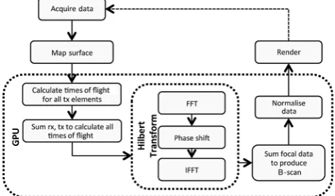
Breaking down Equations (1) and (3) into smaller components allows for the removal of any dependency existing between operations, making the algorithm a suitable candidate for execution over the GPU, which has been shown for a planar interface[8]_. Figure 3 illustrates this process for a non-planar surface where all time-critical operations are performed on the graphics hardware.

4. Ultrasonic surface mapping

The mapping of a surface profile can be achieved through standard ultrasonic techniques, where the pulse-echo signal is used to determine the distance from the ultrasonic source to the first significant signal. This basic principle has led to the development of a wide variety of sensors, commonly used for proximity and distance measuring[11]_{. In its most basic form, a} single element transmits ultrasonic energy into the material before receiving the reflected signal. From this, the time to the first signal response can be converted to distance. Repeating the process for all elements of the aperture allows for the surface of the profile to be mapped, provided the ultrasonic energy is received by the transmitting element and not reflected away. The acquisition of the full matrix of data allows the pulse-echo signal from each transmitting element to be retrieved by taking the diagonal of the data.

Ultrasonic measurements can be obtained from a simple threshold method (STM), where the range distance is determined from the pulse-echo signal at the point where it exceeds an arbitrary threshold typically set by the user. This has the benefit of ease of implementation, but requires user intervention to adequately determine the best value at which to set the threshold[12]_{. It is also} subject to some error since the point at which the threshold is broken occurs after the actual distance to be measured. This error is frequently ignored[13]_{. While some effort towards automation has} been researched, it is more common to approach the problem using the threshold-crossing method (TCM).

4.1 Threshold crossing method

The threshold crossing method was first developed for range measurements as an attempt to solve the problem using digital signal processing techniques in preference to setting an arbitrary threshold value[14] _{and operates on the principle of subtracting} the delay where the greatest match occurs between the echo signal and the reference signal[13]_{. For ultrasonic inspection, this} method first requires an input signal to be modelled, which for this experimental configuration is a five-cycle Gaussian window with sufficient sample points to match the return signal. This can be created through Equation (4), where the length (N) is calculated from 5(1=ProbeFrequency)SampleFrequency:

w n

( )

−1₂α n N/2

⎛ ⎝⎜ ⎞⎠⎟

2

where−N

2 ≤n≤N2,α =2.5

...(4)

It is then necessary to find the envelope of the pulse-echo signal, which can be calculated using the Hilbert transform or some other envelope detection method, and to normalise this response, allowing the amplitude scale to match the input signal. Once computed, the process takes the following steps:

q _{Find the sample point closest to the half amplitude for the input}

signal (is) and the return signal (rs).

q _{Subtract the input signal sample point (is) from the return signal}

sample point (rs).

q _{Calculate the time interval to this new sample point (rs – ri) to}

determine an estimate for the start of the signal.

This approximation can be resolved to a higher level of accuracy by exploiting an iterative algorithm that loops until the required level of accuracy has been obtained[13]_.

4.2 Discussion

Range measurements from a single pulse-echo dataset (the FMC diagonal) is usually insufficient for mapping a geometric profile in all but the simplest of cases, and for better positional accuracy it is often necessary to obtain several pulse-echo/pitch-catch measurements. The use of ultrasonic rangefinders is commonplace in mobile robotic systems, where positional accuracy is obtained from several pulse-echo measurements allowing for surroundings to be mapped in 3D space[15]_{. Illustrated in Figure 4, the concept} has been developed further for this work by obtaining an addition pulse-echo measurement from the neighbouring active transducer element. The correct positioning of a reflector can then be deduced by triangulation, using the three length measurements: the pulse-echo measurement (t) from the transmitting element; the pitch-catch measurement (r) obtained from transmitting on element n and receiving on element n + 1; and the inter-element spacing p (or aperture pitch). From these measurements, migration from xt, zt

to xm, zm is determined from Equations (5) and (6). The process is

repeated for all elements in the array:

xm=xt+

(

)

2pr ...(5)

zm= xm2_−t2 _...(6) The method outlined above combined with the rangefinder principle was explored in this paper for computational efficiency and accuracy in measurement detections. In the case that the geometry is already known, better results may be accomplished by applying a curve fitting algorithm to the profile coefficients, allowing for interpolation of sample points to a higher degree of accuracy[7]_{. Alternatively, the focal requirements may be} pre-calculated ahead of the inspection and retrieved by determining the

transducer’s encoded position at the time of inspection, or obtaining better results through the use of a laser measuring device or a flexible array transducer, providing the benefit of using positional sensors to accurately measure the surface[3]_.

Figure 5 shows the profiles of a non-planar interface, where

z = sin(2πx/40) and z = 2sin(2πx/40), that have been ultrasonically

mapped using the method discussed. It can be observed (in (a) and (c)) that the ability to adequately ultrasonically map the surface is hindered near the trough of the profile and linear interpolation (as shown in (b) and (d)) is required to determine additional interface data points for consideration by the imaging algorithm.

5. Experimental configuration

The focusing algorithm was demonstrated on an experimental data acquisition and post-processing system consisting of:

q _{A data acquisition system controlled by the MicroPulse 5PA}

array controller as manufactured by Peak NDT, Derby. The system contained separate transmit and receive lines per channel and facilitated the use of parallel and sequential transmission techniques. The data acquisition rate of this system via Ethernet was established as approximately 35 MB/s according to the manufacturer’s specification.

q _{A GE 32-element linear array transducer with a 5 MHz central}

frequency and aperture pitch of 1 mm. Data was sampled at a rate of 50 MHz with an 8-bit amplitude resolution and a PRF of 5 KHz.

q _{A Windows 7 desktop-based PC containing two Quadcore 3 GHz}

CPUs and the NVIDIA Tesla C2075 graphics card equipped with 448 CUDA cores and 6048 MB of GDDR5 memory with connection to the MicroPulse via Ethernet, with communication over transmission control protocol/internet protocol sockets.

Two test specimens were imaged of dimensions 120 × 60 × 20 mm and longitudinal velocity of 5981 m/s, with surface profiles of

z = sin(2πx/40) and z = 2sin(2πx/40), containing multiple 1 mm

side-drilled holes along a horizontal plane relative to the normal at a depth of 30 mm. A perspex shoe of depth 25 mm was used to simulate a water path. These test specimens are shown in Figures 6 and 7.

6. Results and discussion

The algorithms were demonstrated on data collected over 32 active transmit and receive elements for each of the test specimens. The system was set to image an area horizontally –15 mm to +15 mm and vertically 25 mm to 35 mm relative to the centre of the aperture and at a resolution of 0.125 mm per pixel, generating images of dimensions 240 × 80 pixels, with reconstruction of the raw data performed in CUDA and C++.

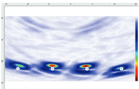
The image of the 2 mm test specimen is shown in Figure 8, where the image is normalised from the peak response with 50 dB gain applied to the signal, to allow maximum signal strength without saturation of the signal. With the algorithms applied, all four side-drilled holes are clearly visible and displayed at the correct lateral position, with a deviation of 0.25 mm in depth positioning (as visible in the right-most side-drilled hole).

In Figure 9, images of the 4 mm test specimen are shown with

Figure 5. Effectiveness of ultrasonic profile mapping to a known geometry (surface) for (a) 2 mm sample, (b) 2 mm sample with linear interpolation, (c) 4 mm sample and (d) 4 mm sample with interpolation. All measurements in millimetres

Figure 6. 2 mm test specimen used for experimental work

Figure 7. 4 mm test specimen used for experimental work Figure 4. Migration of pulse-echo measurements to correct

migrated position, where (t) is the pulse-echo measurement to the first reflector, (r) is the pitch-catch measurement from the first reflector to the neighbouring element and (p) is the inter-element spacing or pitch. An initial position xt, zt is assumed

50 dB gain, again normalised against the peak response. Here, the algorithm performed well for correct lateral placement within the image but depth differences were more pronounced, with the deviation being just over 0.25 mm. In both cases, differences in depth positioning were attributed to the sample rate and transducer configuration, whereby an error of one sample point is equivalent to approximately 0.25 mm and the one-half wavelength measurement is 0.6 mm.

To adequately assess the capability of this work for real-time inspection of complex geometries of an unknown profile, the performance (measured in milliseconds) was recorded for each profile. Data acquisition and processing times remained constant throughout each experiment and the system was shown to be capable of data acquisition, profile mapping and TFM post-processing of the raw data through a dual-layer medium at a rate of 30 frames per second, as shown in Table 1, allowing for real-time and rapid inspection of complex components.

Table 1. Time taken to acquire, map and process data at various configurations. All timings are recorded in milliseconds (ms), with conversion to frames per second (FPS) provided in the final row

Time

Acquire data 10 ms

Map surface 3 ms

Processing 20 ms

Total 33 ms

FPS 30

7. Conclusion

This paper has introduced an optimisation method applicable to FMC acquired data that allows for the computational complexity to be reduced by utilising a look-up table to store the time-of-flight calculations for all transmitting elements, allowing all other time-of-flight combinations to be determined from this single dataset. This technique was applied to imaging through a complex geometry to determine its effectiveness.

A method was then presented that allowed for rapid ultrasonic profile mapping of a complex geometry from the acquired FMC data, where lateral positioning of the profile mapped geometry was corrected by contributions from additional receive elements.

An experimental system was then developed, which showed that rapid post-processing of FMC acquired data is possible from these principles and that the system was able to work with geometries of an unknown profile.

As shown in Equation (3), the TFM algorithm requires four path calculations per transmit/receive combination when focusing through a dual layer. For the experimental configuration, this equates to 39, 321, 600 (322 _{× 2 × 240 × 80) path calculations to} generate a single B-scan image. Through the advanced optimisation techniques described in this paper and through execution of code over the GPU, the system was effectively capable of performing the equivalent of 1, 966, 080, 000 path calculations per second (where post-processing was determined as 20 ms or 50 FPS, as shown in Table 1).

From this work it was shown that real-time TFM inspections were possible for complex components of unknown geometry, with low implementation and development costs.

Acknowledgements

This work was completed in partnership with TWI NDT Validation Centre (Wales), Swansea Metropolitan University, the University of Wales and the Prince of Wales Innovation Scholarship scheme (POWIS).

References

1. R/D Tech, ‘Introduction to phased array ultrasonic technology applications’, R/D Tech guideline, Advanced Practical NDT Series, R/D Tech Corp, 2004.

2. C Holmes, B Drinkwater and P Wilcox, ‘Post-processing of the full matrix of ultrasonic transmit-receive array data for non-destructive evaluation’, NDT&E International, 38 (8), pp 701-711, 2005.

3. A J Hunter, B W Drinkwater and P D Wilcox, ‘Autofocusing ultrasonic imagery for non-destructive testing and evaluation of specimens with complicated geometries’, NDT&E International, 43 (2), pp 78-85, 2010.

4. J Verkooijen and A Boulavinov, ‘Sampling phased array: a new technique for ultrasonic signal processing and imaging’, Insight – Non-Destructive Testing and Condition Monitoring, 50 (3), pp 153-157, 2008.

5. D Gabor, ‘Theory of communications’, Proc IEEE, 93, pp 429-457, 1946.

6. K Riley and P Hobson, Essential Mathematical Methods for the Physical Sciences, Cambridge University Press, 2011. 7. M Weston, P Mudge, C Davis and A Peyton, ‘Time-efficient

auto-focusing algorithms for ultrasonic inspection of dual-layered media using full matrix capture’, NDT&E International, 47, pp 43-50, 2012.

8. M Sutcliffe, M Weston, B Dutton, K Donne and P Charlton, ‘Real-time full matrix capture for ultrasonic non-destructive testing with acceleration of post-processing through graphics hardware’, NDT&E International, 51, pp 16-23, 2012.

9. G Hager and G Wellein, Introduction to High-Performance Computing for Scientists and Engineers, CRC Press, 2010.

Figure 8. Imagery of 2 mm test specimen. All dimensions in millimetres, with 50 dB colour pallet range

10. D Ryan, History of Computer Graphics, Dlr Associates Series, Authorhouse, 2011.

11. C Phanisri, S Chandrasekhara, A Sastry, G T Rao, N Balasubrahmanyam and D S Murty, ‘Ultrasonic surface contour mapping system’, ESA, pp 124-127, 2008.

12. D Mariloli, C Narduzzi, C Offelli, D Petri, E Esardini and A Taroni, ‘Digital time-of-flight measurements for ultrasonic sensors’, IEEE Transactions on Instrumentation and Measurement, 41, pp 93-97, 1992.

13. M Parrilla, J J Anaya and C Fritsch, ‘Digital signal processing techniques for high accuracy ultrasonic range measurements’, IEEE Transactions on Instrumentation and Measurement, 40 (4), pp 759-763, 1991.

14. D T Gibbons, D H Evans, W W Barrie and P S Cosgriff, ‘Real-time calculation of ultrasonic pulsatility index’, Medical & Biological Engineering & Computing, 19 (1), pp 28-34, 1981. 15. B Barshan and D Ba, ‘Comparison of two methods of

surface profile extraction from multiple ultrasonic range measurements’, Measurement Science and Technology, 11 (6), pp 833-844, 2000.