Article
1
The Effect of Temporal Gradient of Vegetation
2
Indices on Early-Season Wheat Area Estimation
3
Using Random Forest Classification
4
Mousa Saei Jamal Abad 1, Ali A. Abkar 2 and Barat Mojaradi 3,*
5
1 Faculty of Geodesy and Geomatics, K. N. Toosi University of Technology, Tehran 19667-15433, Iran;
6
7
2 Faculty of Geodesy and Geomatics, K. N. Toosi University of Technology, Tehran 19667-15433, Iran and
8
AgriWatch BV, Enscede, the Netherlands ; [email protected]
9
3 Department of Geomatics, School of Civil Engineering, Iran University of Science and Technology, Tehran,
10
Iran ; [email protected]
11
* Correspondence: [email protected]; Tel.: +98-912-215-2274
12
Abstract: The early-season area estimation of the winter wheat crop as a strategic product is
13
important for decision makers. Classification of multi-temporal images is an approach which is
14
affected by many factors like appropriate training sample size, proper frequency and acquisition
15
times, vegetation indices (VIs) type, temporal gradient of spectral bands and VIs, appropriate
16
classifier and missed values because of cloudy conditions. This paper addresses the impact of
17
appropriate frequency and acquisition times and VIs type along with the spectral and VI gradient
18
on random forest (RF) classifier when missed values exist in multi-temporal images. To investigate
19
the appropriate temporal resolution for image acquisition, the study area was selected on an
20
overlapping area between two LDCM paths. In our developed method, the miss values of cloudy
21
bands for each pixel are retrieved by the mean of k-nearest ordinary pixels. Then the multi-temporal
22
image analysis is performed by considering different scenarios provided by decision makers in
23
terms of desired crop types that should be extracted at early-season in the study areas. The
24
classification results obtained by the RF decrease by 1.6% when temporally missed values retrieved
25
by the proposed method, which is an acceptable result. Moreover, the experimental results
26
demonstrated that if temporal resolution of Landsat 8 increased to one week the classification task
27
can be conducted earlier with almost better results in terms of OA and kappa. The impact of
28
incorporating VIs along with the temporal gradients of spectral bands and VIs as new features in
29
RF demonstrated that the OA and Kappa are improved 3.1% and 6.6%, respectively. Furthermore,
30
the obtained result showed that if only one image from seasonal changes of crops is available, the
31
temporal gradient of VIs and spectral bands play the main role to discriminate remarkably wheat
32
from barley. The experiments also demonstrated that if both wheat and barley merge to a single
33
class the crop area can be estimated two months earlier with 97.1 and 93.5 in terms of OA and kappa,
34
respectively.
35
Keywords: Wheat classification; Random Forest; Spectral gradient difference; Vegetation indices
36
37
1. Introduction
38
The global demand for food will increase due to increasing of the global population in this
39
century [1]. It is therefore necessary to accurately estimate the crop area to determine if the demand
40
for food can be met [2]. Farmers usually decide to change the crop type of their agricultural fields
41
due to the regional demand and drought condition. Therefore, the cultivated area of a given crop
42
alters from a growing season to next season. Consequently, early-season crop area forecasting, in
43
particular wheat crop, is an essential information for policy makers to manage yields for domestic
44
use, imports or exports.
45
The classification of remotely sensed data can provide regional distribution of individual crop
46
types for government agencies [3,4] and decision makers of commodity trade. Evidently, the
47
classification of agricultural crops using only one image captured at a given date has significant
48
shortcomings [5]. Firstly, the crop types may have different growth stages and secondly, different
49
crops may have similar spectra (e.g. wheat and barley in this case study) during the growing season
50
in a complex agricultural area [6]. It is therefore difficult to distinguish crop types at a certain point
51
in the growth cycle by an image in a given time. In contrast, multi-temporal images provide temporal
52
signatures of crops and represent the growth cycle by capturing data during the growing season [7].
53
Therefore, the temporal signatures of crops may be considered to discriminate crop types [8], and
54
maps of cropland distributions are usually obtained by the supervised classification of
multi-55
temporal images throughout the growing season [9,10]. A significant advantage of using
multi-56
temporal data is that the proportions of different crop types can be discriminated using the spectral
57
differences at different points in the growing season [6,11,12]. Recently, crop areas from non-crop
58
areas have been separated by detecting changes in greenness using time-series normalized difference
59
vegetation index (NDVI) data in [13]. Moreover, an approach based on object-based Normalized
60
Difference Vegetation Index (NDVI) time series analysis is used for regional-scale mapping of
61
agricultural land-use systems [14]. The crop area in early-season was also determined using
62
enhanced vegetation index (EVI) of multi-temporal Moderate Resolution Imaging Spectroradiometer
63
(MODIS) in [11,15]. In their study, the green-up rate of the crop canopy, i.e. the accumulated
64
difference of two consecutive images, is used. The obtained results indicated that multi-temporal
65
remote sensing approach could be used with confidence in early-season crop area prediction at least
66
one to two months ahead of anthesis. Moreover, with increasing number of images, applying
67
different VIs and their differences, the training sample size increases dramatically to overcome the
68
curse of dimensionality for supervised classification [16]. In the study which conducted by [17]
69
different data types including reflectance data, spectral indices, texture indices and DEM features are
70
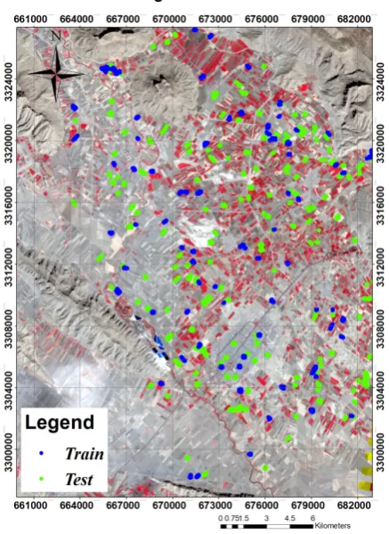
used in a combined random forest (RF) and object bases image analysis scheme for agricultural area
71
mapping. But these approaches require cloud-free imagery and processing of multiple images is
72
prohibitive for operational implementation over large areas. In this regard, acquiring such frequent
73
cloud-free imagery is a serious limitation in estimating crop area [18,19]
74
Indeed, classification of multi-temporal images is a challenging task which is affected by many
75
factors that limit the accuracy. In particular, these issues are appropriate training sample size, proper
76
frequency and acquisition times and suitable VIs. The effect of these factors also depends on the
77
choice of the classifier [20]. Some studies are conducted to address some of these issues[21-24]. For
78
example, the optimal number and dates of images for land cover classification are identified with
79
feature importance yielded by RF classifier on remote sensing time-series [25]. In another study the
80
sensitivity of the RF classification to select training sample points, including sample size, spatial
81
autocorrelation and proportions of classes within the training sample were investigated [21]. In [26]
82
the effect of the time series length on crop mapping is investigated. In this study RF is used to
83
calculate the important scores for VIs and Jeffries –Matusita (JM) distance is used to measure class
84
separability for each time series. In a comprehensive study also five strategies that can be applied to
85
high resolution multi-temporal optical imagery to produce accurate crop type maps have been
86
selected and benchmarked at the global scale [27]. These strategies are RF, support vector machine
87
(SVM) with a redial basis function kernel, Dempster–Shafer fusion of the previous approaches, best
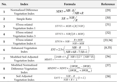
88
classifier with a mean-shift smoothing, best classifier with a temporal regular resampling. The
89
obtained classification results on the 12 test sites over the globe demonstrated that RF achieved
90
superior results. The RF also is used for winter wheat mapping by multi temporal images of LDCM
91
and Gao Fen 1 satellites [28].
92
In aforementioned circumstances, the study of optimal number of images to find critical
93
acquisition times and temporal resolution along with VIs and their gradient is necessary. This paper
94
will address to this issue that how much importance the temporal resolution of image acquisition for
95
multi temporal images classification and what happen when temporal resolution of Landsat 8
96
increase to one week? For this purpose, the study area is selected on overlap area between two
Landsat paths. Moreover, missed values problem in cloudy times is another matter which limits the
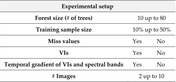
98
application of multi-temporal image classification. Indeed, many pixels of training or non-training
99
data are ignored if only one cloudy image exist in the time series. Although considerable research has
100
been previously conducted on the time-series classification, the problem of miss values caused by
101
cloudy pixels in such images is still an issue to which less attention has been paid. Indeed, the pixels
102
of data are either cloudless pixels or miss data pixels associated with miss values (i.e. bands with no
103
data) due to the availability of cloudy images in time series. One of the main problems in the
multi-104
temporal image classification is that some pixels of training/testing areas may be covered by cloud
105
during the analysis period. Hence, those pixels are ignored and neither incorporated as training data
106
in the classifier learning process nor as test data for the classification accuracy. On the other hand,
107
the rest of cloudy pixels cannot be classified by classifier. This paper remedies this problem for those
108
training/test data and for rest of cloudy pixels by retrieve of the miss values trough k-nearest neighbor
109
cloudless pixels. This paper proposes a method to retrieve the miss values and study the effect of
110
miss value retrieval of training data on classification results of multi temporal images.
111
This paper also addresses the impact of the appropriate frequency and acquisition times and VIs
112
along with the spectral and VI gradient on the RF classifier when miss values are available in the
113
multi-temporal images. The objective of this paper is therefore to investigate the practical
114
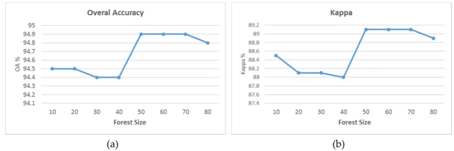
considerations of the multi-temporal image classification approach for consultants and agronomists.
115
The specific goals of this study are: (1) To assess the effect of miss values in training areas, due to
116
cloudy times, on RF classification learning; (2) To determine the appropriate data acquisition times
117
and temporal resolution; (3) To assess the effect of VIs and their temporal gradient along with
118
temporal gradient of spectral bands in different times; and (4) To determine the optimum number of
119
classes to be distinguished in early season. To our knowledge, there are currently no other
120
comprehensive assessments of multi-temporal image classification which takes into consideration
121
these practical aspects.
122
2. Materials and Methods
123
2.1. Study Area and Data: The study area is an agricultural region with an area of 755 km2,
124
located between latitudes 29° 49'–30° 05'N and longitudes 52° 39'–52° 55'E, in Southwest of Iran
125
(Figure 1. The area has various climates during the growing season and is covered by different
126
vegetation, soil, and rocky terrain types. The study area is situated on overlapping area between two
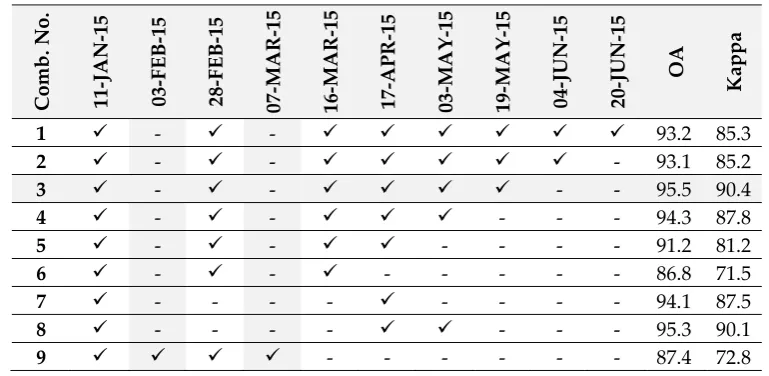
127
paths of 162 and 163, which is covered by 26 scenes of Landsat Data Continuity Mission (LDCM) data
128
captured from 8 Nov 2014 until 26 May 2015 during growing season. In this regard, the temporal
129
resolution in the study area increases from 2 weeks to one week to investigate the appropriate
130
temporal resolution for image acquisition.Among all images, 10 images having less than 20% cloud
131
in the study area are selected which 8 images belonging to path 162 and 2 images to path 163. The
132
acquisition times of these images are given in Table 1.
133
Table 1. Acquisition times of images.
134
Image No. Acquisition Date Image No. Acquisition Date T1 11-JAN-15 T6 17-APR-15
T2 03-FEB-15 T7 03-MAY-15
T3 28-FEB-15 T8 19-MAY-15
T4 07-MAR-15 T9 04-JUN-15
T5 16-MAR-15 T10 20-JUN-15
135
Figure 1. The study area situated in the overlap area between two paths 162 and 163 of LDCM.
137
The training data also were captured in 264 agriculture fields. The spatial distribution of the
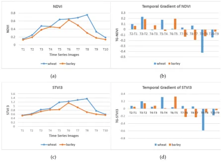
138
training and test areas for the three classes of wheat, barley and other-classes are given in Figure 2
139
and Table 2. As shown, training and test data are selected in disjoint agricultural fields to consider
140
real situation.
141
Figure 2. The spatial distribution of the training and test data for three classes of Wheat, Barley and
142
Table 2. The number of training and test data in the study area.
144
Class # of training fields # of test fields # of training pixels # of test pixels
Wheat 128 280 559 1265
Barely 15 51 93 307
Other 121 252 1419 3027
2.2. Methodology
145
As mentioned above, the classification of multi-temporal images is affected by many factors such
146
as miss values in cloudy images, optimum training sample size, proper frequency and acquisition
147
times that limit the accuracy. Moreover, extraction of appropriate features (e.g. temporal gradient)
148
from the temporal signatures of crop types along with suitable times such that discriminate crops are
149
two major issues that should be considered in the multi-temporal image classification. In this regard,
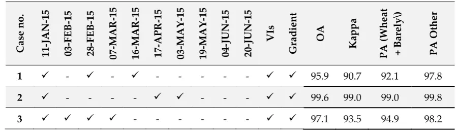
150
different features like VIs and the temporal gradient of VIs and spectral bands are taken into account
151
as new features. To address aforementioned issues, we developed following methodology (Figure 3).
152
153
Figure 3. Flow chart describing the method developed in this study for multi-temporal image
154
classification
155
Step 1: A set of images with acceptable cloud percent, 20% in this study, is selected from input
156
time-series images. Radiometric correction is then conducted on the selected images (i.e. 10 images
157
for this study area) and cloudy pixels in each image are set to no data as missed values for all bands.
158
Hence, for each pixel, a feature vector with a dimension of 80 elements (8×10) is achieved.
159
Step 2: The missed values problem limits the use of training/test data to learn the classifier and
160
the rest of cloudy pixels also cannot be classified in the imaging scene. To overcome this shortcoming
161
for ground data, the bands of a pixel corresponding to cloudy times in a given training/testing class
(e.g. wheat), which contain no data are removed from the feature vector and flagged as cloudy pixels.
163
The corresponding bands from the feature vector of the cloudless pixels of that class are also removed
164
(i.e. the corresponding bands of cloudy times are removed in cloudless pixels of that class) to achieve
165
the same dimensionality with the cloudy pixels. In the reduced multi-dimensional feature space, for
166
each cloudy pixel, k-nearest neighbor cloudless pixels are then found. Therefore, the bands of those
167
pixels with no data are reconstructed by mean of k-nearest cloudless pixels to yield a feature vector
168
with full dimensionality. In other words, the miss values of cloudy bands are filled with the mean of
169
k-nearest from cloudless pixels which are spectrally similar to cloudy pixels in feature space. This is
170
also conducted for the whole cloudy pixels of the scene after the appropriate multi-temporal
171
classification model is selected.
172
Step 3: After miss value retrieval, the VIs are generated. In the current study 9 indices including
173
NDVI, SAVI, SR, EVI, STVI1, STVI3, STVI4, MSAVI1 and MNDVI are generated based on the
174
corresponding equation listed in Table 3, as new features.
175
Table 3. Remote sensing vegetation indices used in this study.
176
No. Index Formula Reference
1 Normalized Difference Vegetation Index
NIR- R
NDVI= NIR R+ [29]
2 Simple Ratio SR =NIRR [30]
3 STress related
Vegetation Index1 STVI1=M IR×
(
R N IR)
[31]
4 STress related
Vegetation Index 3 STVI3=NIR R
(
+MIR)
[32]
5 STress related
Vegetation Index 4 4
R MIR
STVI NIR
NIR MIR
×
= −
+ [33,34]
6 Enhanced Vegetation
Index 2.5
–
6 7.5 1
NIR
E R
NIR R B
VI
+
= × − + [8,35]
7 Modified Soil Adjusted Vegetation Index
(
)
(
)
(
2 1? 1 2 ? ?)
2
NIR NIR NIR R
MSAVI= + + [36]
8
Modified Normalized Difference Vegetation
Index
(
)
(
min)
– max
max
SWIR SWIR
MNDVI NDVI
SWIR SWIR
= ×
+
[37]
9 Soil Adjusted
Vegetation Index (1 )
NIR R
SAVI L
NIR R L
−
= +
+ + [38]
177
Step 4: Because temporal signature plays an important role in the interpretation of the growing
178
steps of crops, temporal gradient is used to quantitatively describe the seasonal change. The temporal
179
gradient of a given spectral band, TGSB, at the ith ( )and jth( ) times are then generated to obtain
180
the temporal changes of crops as follows.
181
182
TGSB ( , ) = SB ( ) - SB ( ) (10)
The temporal gradients of VIs, TGVI, are also computed and considered as new features, which
183
means for a given VI at the ith ( )and jth( ) times, a set of VI gradients in time sequence is generated
184
as follows:
185
186
TGVI ( , ) =VI ( ) - VI ( ) (11)
Step 5: The RF algorithm is conducted to explore the achieved features including spectral bands
187
at different times, VIs and their temporal gradients to yield an ensemble of decision trees. As
188
mentioned, 8 images from path 162 and 2 images from path 163, having less than 20% cloud cover
are selected. Therefore, for each pixel, a feature vector is obtained that includes spectral bands, VIs
190
along with their temporal gradients. To investigate the effect of multi-temporal image classification
191
issues by the RF classification, different scenarios are considered according to Table 4.
192
The RF algorithm can generally handle high dimensional data and use a large number of trees
193
in the ensemble. In RF, each tree in the forest is built and tested independently from other trees.
194
During training, each tree receives a new bootstrapped training set generated from the original
195
training set by subsampling with replacement [39]. Those samples which are not included during the
196
training of a tree are called Out-Of-Bag (OOB) samples of that tree. These samples can be used to
197
compute the Out-Of-Bag-Error (OOBE) of the tree as well as the ensemble which is an unbiased
198
estimate of the generalization error [40-42].
199
In the experiments, replacement and OOB are set to 15 times and 33%, respectively. First, the
200
optimum number of training sample size along with the number of trees are investigated. Then, the
201
effect of each issue is assessed to achieve an appropriate model for the multi-temporal classification.
202
Table 4. The different scenarios for the RF classification.
203
Experimental setup
Forest size (# of trees) 10 up to 80
Training sample size 10% up to 50%
Miss values Yes No
VIs Yes No
Temporal gradient of VIs and spectral bands Yes No
# Images 2 up to 10
3. Results and Discussion
204
Indeed, decision makers aim at achieving crop area from remotely sensed data in earlier season
205
with appropriate accuracy. Therefore, according to Table 5, based on the desired classes two cases of
206
classification are determined by the decision makers.
207
Table 5. Two cases of classification.
208
Case # of classes desired classes
1 3 wheat, barely, other
2 2 (wheat & barely),other
3.1 Experiment 1: Optimum Training Sample Size
209
In this experiment the sample size of the training data, set to 10% up to 50% without considering
210
missed values and only spectral bands of 8 images captured on path 162, without their gradient and
211
VIs are used for classification. The RF classification is performed with 15 times replacement and with
212
50 trees (forest size) in case 1. The averages of the overall accuracy (OA) and Kappa coefficient [43]
213
are computed and given in Figure 4.
Figure 4. Overall accuracy and Kappa coefficient changes to obtain optimum training sample size.
216
With increasing training sample size, the OA and the Kappa coefficient are improved (Figure 4).
217
This improvement is not remarkable when the training sample size become more than 30%. Hence,
218
we selected 30% as appropriate training size due to the cost consuming of filed works.
219
3.2 Experiment 2: Optimum Forest Size
220
Most of experiments used RF classification are conducted with the large number of trees which
221
is time consuming[26,44]. Hence, the optimum forest size for each dataset should be investigated and
222
determined. For this purpose, after achieving the optimum sample size in experiment 1, the optimum
223
forest size is also investigated through increasing trees from 10 up to 80 trees. In this experiment, the
224
RF classification is also conducted with 15 times replacement in case 1 using only the spectral bands
225
of all images. The average values of OAs are given in Figure 5. As demonstrated in Figure 4, the OA
226
becomes almost steady when the number of trees exceeds 50. Hence in this dataset, the optimum
227
forest size and optimum number of training sample size set to 50 trees and 30%, respectively.
228
229
(a) (b)
Figure 5. Effect of the number of trees on (a) overall accuracy (OA) and (b) Kappa coeficient
230
3.3 Experiment 3: The Effect of Miss Values in the Training Data
231
In fact, the pixels of ground data in some images are cloudless while at other times they may be
232
cloudy. In multi-temporal image classification, keeping these pixels is valuable in terms of being time
233
and cost consuming. Moreover, the classification of those pixels which have missed values due to the
234
cloudy times is important when multi-temporal images are used. As mentioned is step2 of the
235
methodology, the miss values (i.e. cloudy bands) of pixels are replaced by the average of k-nearest
236
cloudless pixels. To investigate the effect of the data retrieval method, the retrieval cloudy pixels of
237
the ground data are incorporated to train the RF. Moreover, the retrieval cloudy pixels also are
238
incorporated in test data and are classified. Table 6 shows that the OA value decreases by 1.6 % due
239
to the retrieval miss values by the mean of k-nearest neighbor algorithm. Therefore, it can be
240
concluded that when miss values in the cloudy pixels are retrieved and classified by the RF classifier,
the certainty of obtaining labels for these pixels are less than those of cloudless pixels. Note that all
242
time-series images are used in this experiment and k is set to 7 in this study.
243
Table 6. The effect of miss values on the overall accuracy in the RF classifier.
244
miss value OA Kappa Product Accuracy wheat
Product Accuracy barely
Product Accuracy others
Yes 93.2 85.3 91.5 51.1 97.7
No 95.4 90.3 96.5 62.6 98.0
3.4 Experiment 4: Appropriate Acquisition Times and Temporal Resolution
245
One of the challenges in using multi temporal data is to provide early information about
246
cultivation area and crop types for decision makers with a few images. Hence, at first only different
247
sequential times of path 162 were selected to assess which acquisition times were suitable for early
248
classification. Then classification was conducted on case 1 using different combinations of acquisition
249
time sequences. The summary of using 8 combinations of acquisition times that yield acceptable
250
results are given in Table 7.
251
Table 7. The (OA) and kappa of the RF classifier using combinations of acquisition times.
252
C o m b . No . 11 -JA N -1 5 03 -F EB-15 28 -F EB-15 07 -M AR-15 16 -M AR-15 17 -AP R -1 5 03 -M AY -1 5 19 -M AY -1 5 04 -JU N -1 5 20 -JU N -1 5 OA Kappa1 - - 93.2 85.3
2 - - - 93.1 85.2
3 - - - - 95.5 90.4
4 - - - - - 94.3 87.8
5 - - - - - - 91.2 81.2
6 - - - - - 86.8 71.5
7 - - - - - - - - 94.1 87.5
8 - - - - - - - 95.3 90.1
9 - - - 87.4 72.8
253
The superior result is obtained in Comb.3 when 6 images are used (Table 7). In contrast, an
254
acceptable accuracy in the early season is obtained for decision makers when only thefirst three
255
images of all images are used (i.e. Comb.6). Moreover, a suitable result is also achieved when only 2
256
images are used (i.e. Comb.7). The results may seem remarkable from the processing time standpoint
257
due to using only 2 images.
258
To demonstrate the effect of increasing the temporal resolution of LDCM to one week, the
259
images of path 163 (i.e. dates 03-FEB-15 and 07-MAR-15) are incorporated into the experiment.
260
Therefore, the temporal resolution of LDCM on case study area (i.e. overlap area of two paths of
261
Landsat 8) increased to one week. The experimental results demonstrated that, in this case study, the
262
one-week temporal resolution of LDCM (i.e. Comb. 9), compared to two weeks temporal resolution
263
of LDCM (i.e. Comb.6) achieved better results in terms of OA and kappa. This is due to the fact that
264
only two images from path 163 captured in the first steps of growing season are included. Moreover,
265
early classification (i.e. 07th of March) with better result can be yield if the temporal resolution of
266
Landsat increases to one week. This is promising so that more images with high temporal resolution
267
like Sentinel2A and Sentinel2B can be employed. Although using a constellation of satellites with
268
high spatial and temporal resolution increases the accuracy, certainly a balance between some factors
269
like ground sampling size, processing time, accuracy and early season crop area estimation should
270
be considered.
3.5 Experiment 5: The Effect of VIs and their Gradient
272
This experiment aims at demonstrating the effect of VIs and their gradients on the classification
273
accuracy improvement and their capabilities to decrease scheduled time for image acquisition. For
274
this purpose, at first NDVI and STVI3 as examples of VIs are considered and temporal signatures of
275
wheat and barley are computed and depicted in Figure 6 for training data. As shown in Fig. 6 wheat
276
and barley have similar reflectance in the early stage of growing, making their discrimination difficult
277
in early season. In contrast to wheat, barley yields faster and loses its chlorophyll almost 3 weeks
278
earlier. Then temporal gradient of wheat and barley is computed and given in Figure 6. Although the
279
temporal signatures of these crops in the first stages of growing is almost the same and have high
280
spectral similarity, as shown in Fig. 6, the temporal gradient at the end of the season can provide
281
appropriate features for better discrimination. In particular, the temporal gradient between images
282
of T6 and T7 which acquired at 17 Apr. and 3 May respectively, could provide the first significant
283
difference between these similar classes for discrimination. In other words, from 17 Apr. to 3 May the
284
wheat stands on the late stage of its grows while barely lost chlorophyll more rapidly.
285
286
(a) (b)
(c) (d)
Figure 6. The NDVI and STVI3 indices and their temporal gradient for: (a) NDVI; (b) STVI3; (c)
287
temporal gradient of NDVI; (d) temporal gradient of STVI3, during growing season.
288
After illustrating the VIs and their temporal gradients, the gradient of spectral bands and the
289
aforementioned VIs (Table 2) along with their temporal gradients (i.e. Eqs. (10 & 11)) are incorporated
290
in the RF classification. Figure 6 and Figure 7 shows the results obtained for 28 combinations of
291
acquisition times when only spectral bands are used. In addition to spectral bands, the effect of
292
incorporating VIs and their spectral gradients obtained by Eq. (10) and Eq. (11) is given in Fig.7 in
293
terms of OA and Kapa coefficient. As demonstrated in Fig. 7 by utilizing the temporal gradient of
294
spectral bands and VIs along with their gradients the OA and Kappa are improved up to 5% and 9%,
295
respectively.
(a)
(b)
Figure 7. The classification results when only spectral bands are used versus spectral bands along with VIs
298
and their gradients are used: (a) overall accuracy (OA). (b) Kapa coefficient
299
Table 8. The overall accuracy (OA), kappa and producer’s accuracy (PA) of appropriate times with
300
their Vis and gradient by the RF classifier.
301
C
o
m
b
. No
.
11
-JA
N
-1
5
03
-F
EB-15
28
-F
EB-15
07
-M
AR-15
16
-M
AR-15
17
-AP
R
-1
5
03
-M
AY
-1
5
19
-M
AY
-1
5
04
-JU
N
-1
5
20
-JU
N
-1
5
VIs
TGVI&TGS
B
OA
Kappa
PA W
h
eat
PA B
arely
P
A
Ot
he
r
1 - - - - - 86.8 71.5 82.4 9.8 95.9
2 - - - - - - 88.1 73.9 83.9 10.9 96.7
3 - - - - - 89.9 78.1 86.8 13.0 98.5
4 - - - - - - - 95.3 90.1 97.7 45.5 99.0
5 - - - - - - - - 96.4 92.3 98.2 49.3 100
6 - - - - - - - 99.3 98.4 99.4 92.5 99.9
From 28 combinations, 3 combinations which incorporate minimum acceptable number of
302
images such that discriminate classes of case 1 in early season are selected for comparison. To
303
demonstrate the impact of VIs and their gradients the OA, Kappa and product accuracies (PA) of
304
classes are given in Table 8. As shown, when VIs added to comb. 1 (i.e. early season with 2 weeks
305
temporal resolution) as new features the OA and Kappa improves 1.3%. While this improvement is
306
1.8% when utilizing TGVI and TGSB. Therefore, the use of VIs, TGVI and TGBS as new features the
307
OA and Kappa improve 3.1% and 6.6%, respectively. Moreover, when VIs, TGVI and TGBS features
308
added in Comb.4 not only improve the OA and Kappa but also the TGVI and TGBS features
309
particularly discriminate barley from wheat and improves the PA of barley 43.2%. In contrast to
310
Comb.4, in Comb.3 the TGVI and TGBS do not improve PA of barley significantly. This is due to the
311
similarity between wheat and barley in the early stage of growing. Therefore, the results
312
demonstrated that the appropriate model is Comb.6 which utilizes only 1 image from the first stage
313
of growing season and two images from seasonal change point of wheat and barley. It is worthy to
314
note that compared to Comb.3 the scheduled time decreases to 07-MAR-15 in Comb.7 and yield better
315
results in terms of OA and kappa when temporal resolution increase to one week (i.e. two images of
316
path 163 are used).
317
3.6 Experiment 6: The Effect of the Number of Classes
318
In practice, the classification of all crop types is time and cost consuming.Also when different
319
scenarios for image classification arise in terms of the number of classes, different classification
320
accuracies can be obtained. Moreover, discriminating two similar classes like wheat and barley
321
demands images from a seasonal change point in the temporal signature of those crops. On the other
322
hand, decision makers are usually demand to get information about the cultivated area in early
323
season even for only one or two crop types. Therefore, the number of desired classes to be determined
324
effect on early season detection by the RF classifier. In this experiment, the RF classification is
325
performed on classification case 2 of Table 5 using the appropriate models obtained through
326
experiment 5 (i.e. Comb.3, Comb.6 and Comb.7 of Table 8). The comparative results are given in Table
327
9. The achieved results demonstrated that, compared to the classification case 1, the classification
328
accuracy increased up to 7% in case 2 in terms of OA (i.e. when two classes of wheat and barley are
329
merged into one class). As a result, when decision makers demand to distinguish cultivate area of
330
both wheat and barley, the Comb.7 is an appropriate model which utilizes 4 images from the first
331
stage of growing season with one weak temporal resolution. In this regard, the crop area (Wheat
332
along with Barely) can be estimated with appropriate results almost two months earlier (Table 9).
333
Table 9. The overall accuracy (OA), kappa and producers’ accuracy (PA) when wheat and barley
334
are merged to one class by the RF classifier.
335
C ase no . 11 -JA N -1 5 03 -F EB-15 28 -F EB-15 07 -M AR-15 16 -M AR-15 17 -AP R -1 5 03 -M AY -1 5 19 -M AY -1 5 04 -JU N -1 5 20 -JU N -1 5 VIs Grad ient OA Kappa PA (Wh eat + B are ly\ ) PA O th er1 - - - - - 95.9 90.7 92.1 97.8
2 - - - - - - - 99.6 99.0 99.0 99.8
3 - - - 97.1 93.5 94.9 98.2
4. Conclusions
336
In this study, multi-temporal images were used to discriminate wheat, barley and other classes
337
by the RF classifier with the aims of using a few images acquired in the early stages of the growing
338
season rather than using those of the entire growing season. In the study area, 10 images from the
339
overlapping area between two over paths of 162 and 163 captured during 6 months were examined.
The experimental results demonstrated that 30% of the data and 50 trees were suitable as the
341
optimum training sample size and forest size, respectively in the study area. The miss values due to
342
the cloudy pixels in multi-temporal images were retrieved by the average of the k-nearest cloudless
343
pixels. The achieved results demonstrated that the OA decreased by 1.6 % due to the retrieval miss
344
values. Therefore, it is concluded that when miss values in the cloudy pixels are retrieved and
345
classified by the RF classifier, the certainty of obtaining labels for these pixels is less than the certainty
346
of labels of cloudless pixels. To determine appropriate acquisition times for identifying
347
aforementioned classes, different combinations of acquisition times were generated and evaluated.
348
The experiments demonstrated that the superior result was obtained when 6 images were used while
349
an acceptable accuracy in early season was gained when only thefirst three images of all images were
350
utilized. To demonstrate the effect of increasing the temporal resolution, the images of path 163 were
351
incorporated into the experiment. The experimental results showed that if temporal resolution of
352
Landsat 8 increased to one week the classification task can be conducted earlier with almost better
353
results in terms of OA and kappa.
354
Furthermore, VIs along with TGVI and TGSB were generated as informative features to
355
discriminate wheat and barley. In this regard, the impact of incorporating these generated features
356
was assessed with the aim of decreasing period of time series and improving the accuracy. The results
357
demonstrated that utilizing these new features improve the OA and Kappa 3.1% and 6.6%,
358
respectively. Furthermore, the obtained result showed that TGVI and TGSB play the main role to
359
discriminate remarkably wheat from barley if only one image from seasonal changes of crops is
360
available. The experiments also demonstrated that if the early season detection of both wheat and
361
barley as one class rather more important than separate them, the crop area can be estimated two
362
months earlier with 97.1 and 93.5 in terms of OA and kappa, respectively.
363
The results obtained by this study are promising such that images with high temporal resolution
364
like Sentinel2A and Sentinel2B can be used to achieve accurate discrimination in the early stage of
365
the growing season. Although using a constellation of satellites with high spatial and temporal
366
resolutions increases the accuracy, a balance between some factors like ground sampling size,
367
processing time, accuracy and early season crop area estimation should be certainly considered.
368
Author Contributions: All the authors listed contributed equally to the work presented in this paper.
369
Conflicts of Interest: The authors declare no conflict of interest.
370
References
371
1.
Godfray, H.C.J.; Beddington, J.R.; Crute, I.R.; Haddad, L.; Lawrence, D.; Muir, J.F.;
372
Pretty, J.; Robinson, S.; Thomas, S.M.; Toulmin, C. Food security: The challenge of
373
feeding 9 billion people. science
2010
, 327, 812-818.
374
2.
Padilla, F.; Maas, S.; González-Dugo, M.; Mansilla, F.; Rajan, N.; Gavilán, P.;
375
Domínguez, J. Monitoring regional wheat yield in southern spain using the grami
376
model and satellite imagery. Field Crops Research
2012
, 130, 145-154.
377
3.
Allen, R.; Hanuschak, G.; Craig, M. History of remote sensing for crop acreage in
378
usda's national agricultural statistics service.
2002
.
379
4.
Pan, Y.; Li, L.; Zhang, J.; Liang, S.; Zhu, X.; Sulla-Menashe, D. Winter wheat area
380
estimation from modis-evi time series data using the crop proportion phenology
381
index. Remote Sensing of Environment
2012
, 119, 232-242.
382
5.
Ghamisi, P.; Plaza, J.; Chen, Y.; Li, J.; Plaza, A. Advanced supervised spectral
383
classifiers for hyperspectral images: A review. IEEE Geoscience and Remote Sensing
384
Magazine (GRSM)
2017
.
6.
Vieira, C.; Mather, P.; McCULLAGH, M. The spectral-temporal response surface
386
and its use in the multi-sensor, multi-temporal classification of agricultural crops.
387
International Archives of Photogrammetry and Remote Sensing
2000
, 33, 582-589.
388
7.
Wardlow, B.D.; Egbert, S.L.; Kastens, J.H. Analysis of time-series modis 250 m
389
vegetation index data for crop classification in the us central great plains.
Remote
390
Sensing of Environment
2007
, 108, 290-310.
391
8.
Cammarano, D.; Fitzgerald, G.J.; Casa, R.; Basso, B. Assessing the robustness of
392
vegetation indices to estimate wheat n in mediterranean environments.
Remote
393
Sensing
2014
, 6, 2827-2844.
394
9.
de Colstoun, E.C.B.; Story, M.H.; Thompson, C.; Commisso, K.; Smith, T.G.; Irons,
395
J.R. National park vegetation mapping using multitemporal landsat 7 data and a
396
decision tree classifier. Remote Sensing of Environment
2003
, 85, 316-327.
397
10.
Langley, S.K.; Cheshire, H.M.; Humes, K.S. A comparison of single date and
398
multitemporal satellite image classifications in a semi-arid grassland. Journal of Arid
399
Environments
2001
, 49, 401-411.
400
11.
Carrão, H.; Gonçalves, P.; Caetano, M. Contribution of multispectral and
401
multitemporal information from modis images to land cover classification. Remote
402
Sensing of Environment
2008
, 112, 986-997.
403
12.
Chen, J.; Lu, M.; Chen, X.; Chen, J.; Chen, L. A spectral gradient difference based
404
approach for land cover change detection.
ISPRS journal of photogrammetry and
405
remote sensing
2013
, 85, 1-12.
406
13.
Zheng, B.; Myint, S.W.; Thenkabail, P.S.; Aggarwal, R.M. A support vector machine
407
to identify irrigated crop types using time-series landsat ndvi data.
International
408
Journal of Applied Earth Observation and Geoinformation
2015
, 34, 103-112.
409
14.
Bellón, B.; Bégué, A.; Lo Seen, D.; de Almeida, C.A.; Simões, M. A remote sensing
410
approach for regional-scale mapping of agricultural land-use systems based on ndvi
411
time series. Remote Sensing
2017
, 9, 600.
412
15.
Lobell, D.B.; Asner, G.P. Cropland distributions from temporal unmixing of modis
413
data. Remote Sensing of Environment
2004
, 93, 412-422.
414
16.
Nitze, I.; Schulthess, U.; Asche, H. Comparison of machine learning algorithms
415
random forest, artificial neural network and support vector machine to maximum
416
likelihood for supervised crop type classification. Proc. of the 4th GEOBIA
2012
,
7-417
9.
418
17.
Lebourgeois, V.; Dupuy, S.; Vintrou, É.; Ameline, M.; Butler, S.; Bégué, A. A
419
combined random forest and obia classification scheme for mapping smallholder
420
agriculture at different nomenclature levels using multisource data (simulated
421
sentinel-2 time series, vhrs and dem). Remote Sensing
2017
, 9, 259.
422
18.
Chen, J.; Jönsson, P.; Tamura, M.; Gu, Z.; Matsushita, B.; Eklundh, L. A simple
423
method for reconstructing a high-quality ndvi time-series data set based on the
424
savitzky–golay filter. Remote sensing of Environment
2004
, 91, 332-344.
425
19.
Potgieter, A.; Apan, A.; Hammer, G.; Dunn, P. Early-season crop area estimates for
426
winter crops in ne australia using modis satellite imagery.
ISPRS Journal of
427
20.
Du, P.; Xia, J.; Zhang, W.; Tan, K.; Liu, Y.; Liu, S. Multiple classifier system for
429
remote sensing image classification: A review. Sensors
2012
, 12, 4764-4792.
430
21.
Millard, K.; Richardson, M. On the importance of training data sample selection in
431
random forest image classification: A case study in peatland ecosystem mapping.
432
Remote sensing
2015
, 7, 8489-8515.
433
22.
Fletcher, R.S. Using vegetation indices as input into random forest for soybean and
434
weed classification. American Journal of Plant Sciences
2016
, 7.
435
23.
Eisavi, V.; Homayouni, S.; Yazdi, A.M.; Alimohammadi, A. Land cover mapping
436
based on random forest classification of multitemporal spectral and thermal images.
437
Environmental monitoring and assessment
2015
, 187, 1-14.
438
24.
Pelletier, C.; Valero, S.; Inglada, J.; Champion, N.; Dedieu, G. Assessing the
439
robustness of random forests to map land cover with high resolution satellite image
440
time series over large areas. Remote Sensing of Environment
2016
, 187, 156-168.
441
25.
Nitze, I.; Barrett, B.; Cawkwell, F. Temporal optimisation of image acquisition for
442
land cover classification with random forest and modis time-series.
International
443
Journal of Applied Earth Observation and Geoinformation
2015
, 34, 136-146.
444
26.
Hao, P.; Zhan, Y.; Wang, L.; Niu, Z.; Shakir, M. Feature selection of time series
445
modis data for early crop classification using random forest: A case study in kansas,
446
USA. Remote Sensing
2015
, 7, 5347-5369.
447
27.
Inglada, J.; Arias, M.; Tardy, B.; Hagolle, O.; Valero, S.; Morin, D.; Dedieu, G.;
448
Sepulcre, G.; Bontemps, S.; Defourny, P. Assessment of an operational system for
449
crop type map production using high temporal and spatial resolution satellite optical
450
imagery. Remote Sensing
2015
, 7, 12356-12379.
451
28.
Liu, J.; Feng, Q.; Gong, J.; Zhou, J.; Liang, J.; Li, Y. Winter wheat mapping using a
452
random forest classifier combined with multi-temporal and multi-sensor data.
453
International Journal of Digital Earth
2017
, 1-20.
454
29.
Rouse JW, H.R., Schell JA, Deering DW Monitoring vegetation, systems in the great
455
plains with erts.
In Proceeding of Third Earth Resources,Technology Satellite
456
Symposium 1, Greenbelt, USA
1974
.
457
30.
Jordan, C.F. Derivation of leaf
‐
area index from quality of light on the forest floor.
458
Ecology
1969
, 50, 663-666.
459
31.
Ridao, E.; Conde, J.R.; Mı́nguez, M.I. Estimating fapar from nine vegetation indices
460
for irrigated and nonirrigated faba bean and semileafless pea canopies.
Remote
461
Sensing of Environment
1998
, 66, 87-100.
462
32.
Pearson, R.L.; Miller, L.D. In
Remote mapping of standing crop biomass for
463
estimation of the productivity of the shortgrass prairie, Remote Sensing of
464
Environment, VIII, 1972; p 1355.
465
33.
Thenkabail, P.S.; Ward, A.D.; Lyon, J.G.; Merry, C.J. Thematic mapper vegetation
466
indices for determining soybean and corn growth parameters.
Photogrammetric
467
Engineering and Remote Sensing
1994
, 60, 437-442.
468
34.
Jafari, R.; Lewis, M.; Ostendorf, B. Evaluation of vegetation indices for assessing
469
vegetation cover in southern arid lands in south australia.
The Rangeland Journal
470
35.
Liu, H.Q.; Huete, A. A feedback based modification of the ndvi to minimize canopy
472
background and atmospheric noise. IEEE Transactions on Geoscience and Remote
473
Sensing
1995
, 33, 457-465.
474
36.
Qi, J.; Chehbouni, A.; Huete, A.; Kerr, Y.; Sorooshian, S. A modified soil adjusted
475
vegetation index. Remote sensing of environment
1994
, 48, 119-126.
476
37.
Nemani, R.; Pierce, L.; Running, S.; Band, L. Forest ecosystem processes at the
477
watershed scale: Sensitivity to remotely-sensed leaf area index estimates.
478
International journal of remote sensing
1993
, 14, 2519-2534.
479
38.
Huete, A.R. A soil-adjusted vegetation index (savi). Remote sensing of environment
480
1988
, 25, 295-309.
481
39.
Freund, Y.; Schapire, R.E. In Experiments with a new boosting algorithm, Icml, 1996;
482
pp 148-156.
483
40.
Leistner, C.; Saffari, A.; Santner, J.; Bischof, H. In Semi-supervised random forests,
484
2009 IEEE 12th International Conference on Computer Vision, 2009; IEEE: pp
506-485
513.
486
41.
Breiman, L. Out-of-bag estimation; Citeseer: 1996.
487
42.
Breiman, L. Random forests. Machine learning
2001
, 45, 5-32.
488
43.
Congalton, R.G.; Green, K.
Assessing the accuracy of remotely sensed data:
489
Principles and practices. CRC press: 2008.
490
44.
Wang, L.a.; Zhou, X.; Zhu, X.; Dong, Z.; Guo, W. Estimation of biomass in wheat
491
using random forest regression algorithm and remote sensing data. The Crop Journal
492