What is the Real Shape of the Hubble Diagram, z = H0*D orz e t H0*
1
?
Analysis of the SN1a Supernovae and Gamma Ray Burst Redshift/Magnitude Data
including the High Redshift Range up to z = 8.1
Laszlo A. Marosi
67061Ludwigshafen, Germany
E-mail: [email protected]
Keywords: Galaxies: distances and redshift, high redshift, Stars: Gamma ray bursts: individual, supernovae: individual, Cosmology: distance scale, observations
Abstract
Analyses of the Hubble diagrams are presented for SN1a supernovae and gamma ray bursts in the redshift ranges z = 0.01–1.3 and 0.034–8.1, respectively. Data are presented on the typical z/μ scale and also on the less common yet increasingly sensitive photon flight time t/(z+1) scale. The primary conclusion is that on the basis of the presently accessible data in the redshift range z = 0.01–8.1, the slope of the Hubble diagram is, or is extremely close to, exponential.
1 Introduction
Hubble's constant (H0) [1], in addition to the cosmic microwave background (CMB) and the
big bang nucleosynthesis, is one of the key pillars of big bang cosmology. It is presumably the most significant cosmological parameter, since it determines the rate of expansion and the age and size of the universe, and influences numerous different parts of cosmology. As indicated by its great significance, the velocity interpretation of H0 has achieved a dogmatic status and
other hypotheses, such as the most discussed rival theory: an energy decrease of starlight with a constant rate, for example, were discarded. However, ongoing results have demonstrated
hitherto unrecognized vulnerabilities in the understanding of the redshift (RS, z) of starlight, which requires careful reevaluation.
H0 is normally determined by direct measurement of the RS of atomic spectral lines emitted
by distant galaxies, leading to H0 = 68.5 (Planck reference set)–73 km s-1 Mpc-1 (Millennium
reference set) as the most probable range of H0.
A further method of determining H0 is offered by the CMB power spectrum [2, 3]. Fitting the
cosmological parameters of the lambda cold dark matter (ΛCDM) model with the cosmological constant to the baryonic acoustic oscillation (BAO) gives H0 = 68 km s-1 Mpc-1,
which is close to the value derived from spectral lines.
This outcome is, however, not unambiguous. The BAO can be fitted with a similar, or even better, certainty using various parameters of the multi-parameter field, H0, ΩM, ΩΛ and w.
It was recently shown that the Einstein–de Sitter (EdeS) model with a zero cosmological constant can fit the CMB data as well as the concordance model. Calculating H0 from
different EdeS models without the cosmological constant gives a value of H0 = 30–40 km s-1
Mpc-1 [4, 5].
This result is fairly surprising. A H0 of 30 km s-1 Mpc-1 is entirely inconsistent with values of
68.5–73 km s-1 Mpc-1. This logical inconsistency between the two extremely different H0
values requires prudent clarification.
A further question emerges from the poor knowledge of the Hubble diagram (HD) in the high RS range of 1 < z < 8. It is commonly acknowledged that the historical scenery to the expansion of the universe can be exactly represented by the concordance model, which makes explicit predictions regarding the shape of the HD.
of the ΛCDM model to the SN1a z/μ data applies to only a limited range of distances. One explanation for this lies in the experimental difficulties involved, because at RSs > ~1.3, the optical light emitted by supernovae progressively dims with distance and exact measurements become difficult.
This constraint on the data has motivated several attempts to obtain cosmological parameters from gamma-ray burst (GRB) observations. GRBs are the most brilliant sources in the universe. They are acquired up to RSs of ~8 and higher, and there is hope that these objects may serve as dependable distance indicators.
A number of endeavors have been made to use GRB data to calculate the HD [12–16], with varying degrees of success. Gupta [16] has shown that by weighting a number of different cosmological models with supernovae and GRB z/μ data, the results slightly favor the ΛCDM model but do not support firm conclusions. All models can fit the data well with a fairly high χ2
probability. Lerner [17] also achieved a similar result and has shown that no single model provides a statistically better fit to the same z/μ dataset than another.
Ongoing work in the high RS range of up to z = 8.1 using mixed SN1a and GRB data [18– 20], or solely GRB data [21], has demonstrated that the slope of the HD is, or is extremely close to, exponential, and this contradicts the expectations of the ΛCDM model.
The aim of the present study is to perform a comparative HD test using SN1a supernova and calibrated, cosmology independent GRB RS/μ data points. In the high RS range, it should be possible to definitively verify whether the HD shows the linear
z = H0D (1)
or the exponential
e
relationship, an issue that is not easily detectable in the z < 1 region. Explaining this important question could set significant limits on the real rate of expansion and on the matter and energy content of the universe.
In Equations (1)–(3), t represents the flight time of the photons (s) from the co-moving radial distance D (cm) to the observer, which is proportional to D (Mpc) as used in the Hubble law.
2 Preparation of Hubble Diagram
The HD is a linear plot of the measured distance (usually Mpc) versus the measured RS, which is often represented on the less sensitive logarithmic RS/ μ scale.
Since the difference between the measured and the calculated data becomes more pronounced on the more sensitive linear scale, in addition to the z/μ HD, a plot of the photon flight time (t) versus RS was used for representation of the HDs. The photon flight time was calculated from
10 * 085 , 3 * 10 * 3 * ) 1 ( 10 18 10 5 / ) 5 ( z c D t (3)
For visualization of the data the t*10-14/z data presentation was chosen.
In addition to the increased sensitivity, an obvious advantage of the t/(z +1) representation is the direct illustration of the shape of the HD, which can be directly compared with the predictions following from Equations (1) and (2).
3 Data Collection and Processing
3.1 Dataset for SN1a Supernovae
The joint light-curve analysis (JLA) data index, the most recent list of 740 spectroscopically affirmed SNIa supernovae with excellent light curves, is believed to currently be the most exact supernovae z/μ database. From these data, 32 binned RS/μ data points were calculated by Betoule et al. [22], which give an exact representation of the 740 data points.
3.2 Processing of SN1a Data
3.3 Dataset for Gamma Ray Bursts
A total of 138 calibrated, cosmology independent GRB z/μ data points collected by Liu and Wei [23] from 557 Union2 compilations were utilized as the starting dataset. Compared with the 2010 data release containing 109 z/μ data points [24], the 2015 dataset contains 30 more data points and the data are more precise, particularly in the low z range.
3.4 Processing Gamma Ray Burst Data
In view of the experimental difficulties in determining the z/μ data, it is likely that in addition to the observed considerable scatter, large datasets taken from different observations and from different sources will contain outliers. If these are not removed in the refinement procedure, they will overwhelm the fit. Any single distant outlier can impose considerable bias in the best fit of the HD and ruin the result. It is therefore important to clean the data by eliminating the outliers and to use these cleaned data for statistical analysis. For this purpose, the data smoothing and for the following identification of outliers, best fit curves were calculated using the empirical potential function
μ = a*zn, (4) which was found in earlier studies to be the best mathematical approximation for describing the slope of the observed z/μ diagrams [18, 19, 25].
3.5 Identification of Outliers: The Grubbs Test
The well-known Grubbs test [26] was used for the identification of erroneous luminosity indicators. The Grubbs test is used to detect outliers in a data set of N values that are nearly normally distributed. Assuming a normal distribution of the sample, as confirmed by the very low skew in Table 1, the test is performed by computing x0, defined as:
1 *
N N STABW G
XO G
x
Mean (5)xo is the suspected outlier;
xMean is the absolute value of the mean of N data points;
N is the number of data points;
STABW is the standard deviation of N values; GG is the Grubbs number.
GG can be found in statistical tables for different levels of confidence and numbers of data
points. For 138 data points, the value of GG is 1.958 at the 95% confidence level. If the value of xo calculated from (μmeasured - μcalculated on basis of the best fit) is found to be greater than the
numerical value of the right-hand side of Equation (5), the data point in question is
discarded. Then, on the basis of the reduced dataset and new a and b coefficients, the
mean and the new STABW are calculated and so on.
The goodness of fit was calculated using the likelihood estimator
N i t calc
calc t obs t
1 ( ) .
.) ) ( . ) (
( 2
2
. (6)
3.6 Luminosity Distances
Luminosity distances were calculated using the ICRAR cosmological calculator [27].
3.7 Data Presentation
Excel and Excel solver were used for data fitting, refinement and data presentation.
4 Results
4.1 Hubble Diagram for SN1a Supernovae in the RS Range 0.0104–1.3 on Logarithmic
z/μ and Linear t/(z+1) Scales
4.1.1 Logarithmic Data Presentation
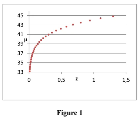
Figure 1 shows the logarithmic z/μ HD for the observed z/μ values (squares) together with the z/μ data points calculated with ICRAR, with H0 = 70 km s-1 Mpc-1, ΩM = 0.295 and w =
Figure 1
Figure 1: Logarithmic z/μ HD for the observed z/μ data (squares) together with the z/μ data points calculated
with ICRAR, with H0 = 70 km s-1 Mpc-1, ΩM = 0.295 and w = −1.018 (triangles) [20, 27]. The fit results are summarized in Table 1 below.
Table 1
SN1a supernovae
Descriptive statistics for the observed z/μ data related to the calculated z/μ.
Valid cases R2 F-test
μobs/μcalc
∑χ2
(μobs-μcalc)
31 0.9994 0.9932 0.0062
Std. deviation (μobs-μcalc)
Variance (μobs-μcalc)
Skew (μobs-μcalc)
Mean (μobs-μcalc) 0.084 0.0072 -1.09 −0.0061
As can be seen from Figure 1 and Table 1 (which represents the difference between the observed and calculated data quantitatively), the two data sets are practically congruent.
4.1.2 Data Presentation on Lineart/(z+1) Scale
In Figures 2 and 3, the corresponding HDs are plotted on the linear t*10-14/(z+1) scale for the observed and calculated μ values.
33 35 37 39 41 43 45
0 0,5 1 1,5
μ
Figure 2 Figure 3
Figure 2: t/(z+1) HD: trendline (solid line), observed data points (dotted line).
Figure 3: t/(z+1) HD: trendline (solid line), calculated data points (dotted line).
(The orange point at z+1 = 2.105 in Figure 2 is obviously an ‘outlier’ and was therefore excluded from the calculation of the goodness of fit indicators.)
Descriptive statistics are summarized in Tables 2 and 3.
Table 2
SN1a supernovae
Data fitting with exponential function, observed data Descriptive statistics t/(z+1)
Valid cases H0 R2 F-test
zobs/zcalc
∑χ2
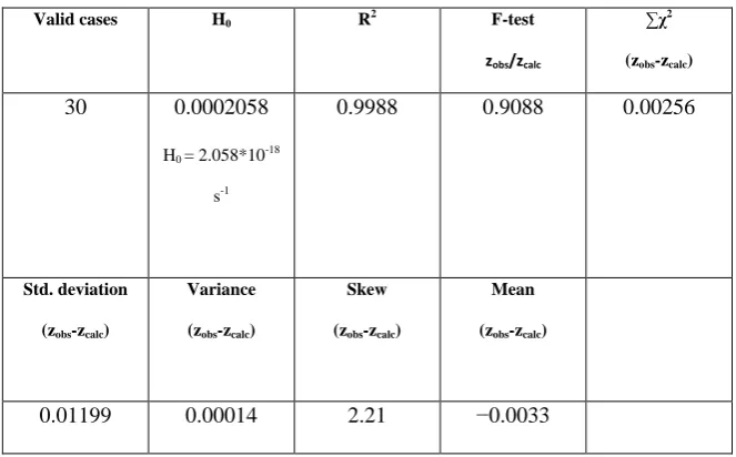
(zobs-zcalc) 30 0.0002058
H0 = 2.058*10-18
s-1
0.9988 0.9088 0.00256
Std. deviation (zobs-zcalc)
Variance (zobs-zcalc)
Skew (zobs-zcalc)
Mean (zobs-zcalc)
0.01199 0.00014 2.21 −0.0033
Table 3
SN1a supernovae
Data fitting with exponential function, calculated data y = e0,0002058x
R² = 0,9988
1 1,2 1,4 1,6 1,8 2 2,2 2,4
0 2000 4000 6000
z +1
t*10-14 sec.
y = e0,0002050x R² = 0,99927
1 1,2 1,4 1,6 1,8 2 2,2 2,4
0 2000 4000 6000
z + 1
Descriptive statistics t/(z+1)
Valid cases H0 R2 F-test
zobs/zcalc
∑χ2
(zobs-zcalc) 31 0.0002050
H0 = 2.05*10-18 s -1
0.99927 0.9236 0.00176
Std. deviation (zobs-zcalc)
Variance (zobs-zcalc)
Skew (zobs-zcalc)
Mean (zobs-zcalc)
0.0089 7.59*10^-5 1.82 0.0032
In the RS range 0–1.3, the HD for the observed data and the HD based on the calculated z/μ data can be described with high accuracy by both the ΛCDM model and the exponential functions z+1 = e0.0002058*t*10^-14 and z+1 = e0.0002050*t*10^-14, respectively. For both the linear and logarithmic scales, the two cases are, within statistical uncertainties, similar.
This result is rather unexpected and probably of an accidental nature that leaves two options open: either, in the low RS range at certain values of the parameters ΩM, Ωʎ, H0 and w, the
shape of the HD is very close to exponential, or, the shape of the observed HD is really exponential not only in the low but also in the high RS range. Measurements including the high RS region are necessary for clarifying this important question.
4.2 Hubble Diagram for Gamma Ray Bursts on Logarithmic z/μ and Linear t/(z+1)
Scales including the High Redshift Range up to z = 8.1
4.2.1 Logarithmic Data Presentation
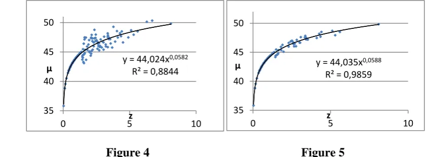
improved the goodness of fit indicators (Tables 5 and 6). The best fit line μ = 44,035*z0.0588 allows a scatter free conversion of the z/μ data into the t/(z+1) scale.
Figure 4 Figure 5
Figure 4: z/μ diagram for the original 138 data points.
Figure 5: z/μ diagram for the 96 cleaned data points.
Table 4
Results of regression with μ = a×zb
Descriptive statistics z/μ for 138 data points
Valid cases a b R2 ∑χ2
(μobs-μcalc)
138 44.024 0.582 0.8844 1.925
F-test
μobs/μcalc
Std. deviation (μobs-μcalc)
Variance Skew (μobs-μcalc)
Mean (μobs-μcalc)
0.4376 0.8057 0.65 0.027 0.073
Table 5
Results of regression with μ = a×zb
Cleaned dataset
Descriptive statistics z/μ for 96 cleaned data points
Valid cases a b R2 ∑χ2
(μobs-μcalc)
96 44.035 0.0588 0.9859 0.1607
F-test Std. deviation Variance Skew Mean
y = 44,024x0,0582 R² = 0,8844
35 40 45 50
0 5 10
μ
z
y = 44,035x0,0588 R² = 0,9859
35 40 45 50
0 5 10
μ
μobs/μcalc (μobs-μcalc) (μobs-μcalc) (μobs-μcalc) (μobs-μcalc)
0.9668 0.2793 0.078 −0.834 −0.0128
4.2.2 Data Presentation on Lineart/(z+1) Scale
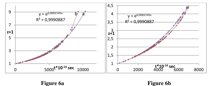
Figure 6a shows a plot of the linear t*10-14/(z+1) HD from the best fit parameter (Table 5) of the observed data (line a) together with the curve inferred from the calculated ΛCDM data with H0 = 70 km s-1 Mpc-1, ΩM = 0.295 and w = −1.018 (line b) [22].
Figure 6a Figure 6b
Figure 6a: Representative t*10-14/(z+1) HD based on 97 statistically verified GRB data points (line a) and the calculated ΛCDM data (line b).
Figure 6b: Section of Figure 6a in the RS range from 1–4.5.
The shape of the HD for the observed data (line a in Figure 6a) is very close to exponential, whilst the ΛCDM model shows systematic deviations from the exponential best fit curve (line b) in Figure 6a):
∑χ2
t (exponential best fit – observed data) = 108, ∑χ2
t (exponential best fit – ΛCDM model) = 791.
The HD diagram on basis of the ΛCDM model with H0 = 70 km s-1 Mpc-1 deviates below the
trendline of the best-fit curve for z + 1 < ~4.5 to the bottom (Figure 6b) and above it for z + 1 > ~4.5 (Figure 6a). These deviations are of a non-statistical nature and thus the ΛCDM model does not reflect the observed exponential slope.
Table 6
y = e0,0002145x R² = 0,9990887
1 3 5 7 9
0 5000 10000
z+1
t*10-14 sec
b a y = e0,0002145x
R² = 0,9990887
1 1,5 2 2,5 3 3,5 4 4,5
0 2000 4000 6000 8000
z+1
Descriptive statistics for the exponential line (a) in Figure 6a based on z
Valid cases H0 R2 F-test
zobs/zcalc
∑χ2
(zobs-zcalc) 96 0.0002145
H0 = 2.14*10-18 s -1
0.9991 0.9584 0.0484
Std. deviation (zobs-zcalc)
Variance (zobs-zcalc)
Skew (zobs-zcalc)
Mean (zobs-zcalc) 0.0434 0.0001 1.098 −0.022
5 Conclusions
A remarkable result of our analysis of the SN1a supernovae data in the RS range 0.0104–1.3 is that on the basis of the z/μ HD, the good fit of the cosmological parameters to the observed data cannot be seen as a definitive proof in favor of the redshift interpretation according to Equation (1). Figures 2 and 3 show that even in the more sensitive t/(z + 1) representation and even on basis of the most accurate JLA data, the slope of the ΛCDM-HD cannot be distinguished from an exponential slope according to Equation (2), which is characteristic for an energy decay with a constant rate. In the RS range < ~1.3, the two curves are practically congruent.
in the whole RS range from z = 0.031–8.1; nevertheless, much more precise data, especially in the high RS range, are required to confirm our results. Due to the work of Swift (The Neil Gehrels Swift Observatory, NASA), the fundamental highlights of GRBs have become better known as of late. A large number of blasts have been seen in the range of 0.034 < z ≤ 8.1, which opens up the possibility of estimating the expansion history back to the formation of the first stars. The hope is justified that this can be achieved with future surveys.
Acknowledgments
The author thanks Dr. Rajendra Gupta and Dr. Eric Lerner for valuable and helpful discussions.
Additional Information
The author declares no conflict of interest
References
[1] Hubble, E. P., 1929, A relation between distance and radial velocity among extra-galactic nebulae, Proceedings of the National Academy of Sciences of the United States of America 15, 167–173.
[2] Jungmann, G., et al., 1996, Cosmological-parameter determination with microwave background maps, Physical Review D 54, 1332.
[3] Zaldarriaga, M., Spergel, D. N. & Seljak, U., 1997, Microwave Background Constraints on Cosmological Parameters, Astro-ph/9702157.
[4] Lineweaver, C. H. & Barbosa, B., 1998, Cosmic microwave background: Implications for Hubble constant and the spectral parameters n and Q in cold dark matter critical density universes, Astronomy & Astrophysics 329, 799–808.
[5] Blanchard, A., Douspis, M., Rowan-Robinson, M. & Sarkar, S., 2003, An alternative to the cosmological ‘concordance model’, Astronomy & Astrophysics 412, 35–44.
[7] Riess, A. et al., 1998, Observational evidence from supernovae for an accelerating universe and a cosmological constant, Astrophysical Journal, 116, 1009.
[8] Schmidt, B.P. et al., 1994, The expanding photosphere method applied to SN 1992am AT cz = 14 600 km/s, Astronomical Journal 107, 1444–1452.
[9]Sorrell, W.E., 2008, Misconceptions about the Hubble recession law, Astrophysics and Space Science 317, 45.
[10] Traunmüller, H., 2014, From magnitudes and redshifts of supernovae, their light-curves, and angular sizes of galaxies to a tenable cosmology, Astrophysics and Space Science 323, 205–211.
[11] Vigoureux, J.-M., Vigoureux, P. & Vigoureux, B., 2008, Cosmological applications of a geometrical interpretation of “c”. International Journal of Theoretical Physics 47, 928-–935, arXiv: 0711.3990 [astro-ph].
[12] Schäfer, B.E., 2006, The Hubble diagram to redshift > 6 from 69 gamma ray bursts, arXiv:astro-ph/0612285.
[13] Izzo, L., Capozziello, S., Covone, G. & Capaccioli, M., 2009, Extending the Hubble diagram by gamma ray bursts, Astronomy and Astrophysics 508, 63–67.
[14] Demianski, M., Piedipalumbo, E. & Rubano, C., 2011, The gamma-ray bursts Hubble diagram in quintessential cosmological models, Monthly Notices of the Royal Astronomical Society 411, 1213–1222.
[15] Cardone, V. F., Capozziello, S. & Dainotti, M.G., 2009, An updated gamma ray bursts Hubble diagram, arXiv: 0901.3194v2.
[16] Gupta, R., 2019, Weighing cosmological models with SN1a and gamma ray bursts redshift data, Universe, 5(5), 102.
[17] Lerner, E., Private communication
[19] Marosi, L.A., 2016, Modelling and analysis of the Hubble diagram of 280 supernovae and gamma ray bursts redshifts with analytical and empirical redshift/magnitude data, International Journal of Astronomy and Astrophysics 6, 272–275.
[20] Vigoureux, J.-M., Vigoureux, D., Vigoureux, P. & Langlois, M., 2018, Analysis of the Hubble diagram of type SNe Ia supernovae and of γ-ray bursts: A comparison between two models, arXiv: 1804.03519 [Physics.gen-ph].
[21] Marosi, L.A., 2019, Extended Hubble diagram on basis of gamma ray bursts including the high redshift range of z = 0,031- 8,1, International Journal of Astronomy and Astrophysics 9, 1–11.
[22] Betoule, M. et al., 2014, Improved cosmological constraints from a joint analysis of the SDSS-II and SNLS supernova samples, arXiv:1401.4064, [astro-ph-CO].
[23] Liu, J. & Wei, H, 2015, Cosmological models and gamma-ray bursts calibrated by using Padé method, General Relativity and Gravitation47, 141,arxiv.org/abs/1410.3960.
[24] Wei, H., 2010, Observational constraints on cosmological models with the updated long gamma ray bursts, Journal of Cosmology and Astroparticle Physics 020, 14.F.
[25] Marosi, L.A., 2013, Hubble diagram test of expanding and static cosmological models: The case for a slowly expanding universe, Advances of Astronomy, Article ID 917104. [26] Grubbs, E., 1950, Sample criteria for testing outlying observations,The Annals of Mathematical Statistics, 21, 27–58.