Including Arbitrary Geometric Correlations into One-Dimensional Time-Dependent Schrödinger Equations

Including arbitrary geometric correlations into

one-dimensional time-dependent Schrödinger

equations

Devashish Pandey1,∗, Xavier Oriols1,∗and Guillermo Albareda2,3,∗

1_{Departament d’Enginyeria Electrònica. Universitat Autònoma de Barcelona. Edifici Q. 08193 Bellaterra.} 2_{Max Planck Institute for the Structure and Dynamics of Matter and Center for Free-Electron Laser Science,}

Luruper Chaussee 149, 22761 Hamburg, Germany.

3_{Institut de Química Teòrica i Computacional (IQTCUB), Universitat de Barcelona, Martí i Franquès 1, 08028}

Barcelona, Spain.

* Correspondence: [email protected] (D.P), [email protected] (X.O), [email protected] (G.A)

Abstract:The so-called Born-Huang ansatz is a fundamental tool in the context of ab-initio molecular dynamics, viz., it allows to effectively separate fast and slow degrees of freedom and thus treating electrons and nuclei at different mathematical footings. Here we consider the use of a Born-Huang-like expansion of the three-dimensional time-dependent Schrödinger equation to separate transport and confinement degrees of freedom in electron transport problems that involve geometrical constrictions. The resulting scheme consists of an eigenstate problem for the confinement degrees of freedom (in the transverse direction) whose solution constitutes the input for the propagation of a set of coupled one-dimensional equations of motion for the transport degree of freedom (in the longitudinal direction). This technique achieves quantitative accuracy using an order less computational resources than the full dimensional simulation for a prototypical two-dimensional constriction.

Keywords: nanojunction; constriction; quantum electron transport; quantum confinement; dimensionality reduction, stochastic Schrödinger equations; geometric correlations

1. Introduction

Nanoscale constrictions (sometimes referred to as point contacts or nanojunctions) are unique objects for the generation and investigation of ballistic electron transport in solids. Studies of such systems have been inspired by the pioneering investigations by Sharvin in the mid-1960s [1]. Today, advances in the fabrication techniques like direct growth of branched nanostructures [2], electron beam irradiation [3], thermal and electrical welding [4] or atomic force microscope [5] have allowed to control the size and composition of nanojunctions for creating devices with desired functionalities. In this respect, a number of nanodevices based on nonjunctions like the single electron transistors [6,7], field effect transistors [8,9] and heterostructure nanowires [10,11] have been recently reported which promise great performance in terms of miniaturization and power consumption.

In the design of these nanostructures, simulation tools constitute a valuable alternative to the expensive and time-consuming test-and-error experimental procedure. Today, a number of quantum electron transport simulators are available to the scientific community [12–16]. The amount of information that these simulators can provide, however, is mainly restricted to the stationary regime and therefore their predicting capabilities are still far from those of the traditional Monte Carlo solution of the semi-classical Boltzmann transport equation [17]. This limitation poses a serious problem in the near future as electron devices are foreseen to operate at the Terahertz (THz) regime. At these frequencies, the discrete nature of electrons in the active region is expected to generate unavoidable fluctuations of the current that could interfere with the correct operation of such devices both for analog and digital applications [18].

A formally correct approach to electron transport beyond the quasi-stationary regime lies on the modeling of the active region of electron devices as an open quantum system [19,20]. As such, one can then borrow any state-of-the-art mathematical tool developed to study open quantum systems [21,22]. A preferred technique has been the stochastic Schrödinger equation (SSE) approach [23–30]. Instead of directly solving equations of motion for the reduced density matrix, the SSE approach exploits the state vector nature of the so-called conditional states to alleviate some computational burden [31].

An example of the practical utility of the SSE, a Monte Carlo simulation scheme to describe quantum electron transport in open systems that is valid both for Markovian or non-Markovian regimes and that guarantees a dynamical map that preserves complete positivity has been recently proposed [32]. The resulting algorithm for quantum transport simulations reformulates the traditional "curse of dimensionality” that plagues all state-of-the-art techniques for solving the time-dependent Schrödinger equation (TDSE). Specifically, the algorithm consists on the solution of an ensemble of single-particle SSEs that are coupled, one to each other, through effective Coulombic potentials [33,34]. Furthermore, the simulation technique accounts for dissipation [35] and guarantees charge and current conservation through the use of self-consistent time-dependent boundary conditions [36–38] that partially incorporate the exchange interaction [39,40]. Solving a large number of three-dimensional (3D) single-particle TDSEs, however, may still be a very time-consuming task. Therefore, the above technique would greatly benefit from the possibility of further reducing the dimensionality of the numerical problem.

It is the purpose of this work to derive and discuss a method that allows to solve the 3D TDSE in terms of an ensemble of one-dimensional (1D) TDSEs. The technique is inspired on the so-called Born-Huang ansatz [41], which is a fundamental tool in the context of ab-initio molecular dynamics that allows to separate fast and slow degrees of freedom in an effective way [42]. Here we consider an analogous ansatz to separate transport and confinement directions. As it will be shown, the resulting technique allows us to include arbitrary geometric correlations into a coupled set of 1D TDSEs. Therefore, while we have motivated the development of this method in the context of the simulation of (non-Markovian) quantum transport in open system, the method presented here could be of great utility in many research fields where the reduction of the dimensionality in quantum systems with geometrical correlations may be advantageous.

The manuscript is structured as follows. In Section2we introduce a Born-Huang-like ansatz that allows to expand the 3D single-particle TDSE in terms of an infinite set of (transverse) eigenstates weighted by (longitudinal) complex coefficients. The equations of motion for the coefficients are found to be coupled and obey a linear (non-unitary) partial differential equation. In Section3we apply the method to a prototypical 2D constriction. Section3.1is devoted to find analytical expressions for the effective potentials that appear in the equation of motion of the coefficients. A discussion on the geometrical dependence of these effective potentials is provided. In Section3.2we illustrate the performance of the method to describe the dynamics of an electron across the 2D nanojunction. In Section4we provide a thorough discussion on the advantages and potential drawbacks of the method. We conclude in Section5.

2. Single-electron time-dependent Schrödinger equation in a Born-Huang-like basis expansion

As we have explained in the introduction, it is our goal to reduce the computational burden associated to the solution of an ensemble of effective single-electron 3D SSE [32]. Therefore, we consider our starting point to be the 3D TDSE of a single (spin-less) electron in the position basis, i.e.:

i ∂

where we have used atomic units, andx,yandzrepresent the three spatial coordinates. In Equation1, H(x,y,z)is the full Hamiltonian of the system:

H(x,y,z) = Tx+Ty+Tz+V(x) +W(x,y,z), (2) which has been assumed to be time-independent for simplicity. The time-dependence on the scalar potentialsV(x)andW(x,y,z)will be discussed in later sections. In Equation2,Tx=−1₂ ∂

2

∂x2 andV(x) are, respectively, the kinetic energy and the scalar potential associated to the longitudinal degree of freedomx, whileTy= −1₂ ∂

2

∂y2 andTz =−12 ∂ 2

∂z2 are the kinetic energies associated to the transversal degrees of freedomyandz. The scalar potentialW(x,y,z)includes any other scalar potential that is not purely longitudinal, which is responsible of making the solution of Equation1non-separable.

It is convenient at this point to rewrite the Hamiltonian in Equation2in terms of longitudinal and transverse components as:

H(x,y,z) =Tx+V(x) +Hx⊥(y,z), (3) whereH⊥x(y,z)is the transverse Hamiltonian defined as:

Hx⊥(y,z) =Ty+Tz+W(x,y,z). (4) An eigenvalue equation associated to the transverse Hamiltonian can now be introduced as follows:

H_x⊥(y,z)φk_x(y,z) =Ek(x)φk_x(y,z), (5)

where Ek_{(x) and φ}k

x(y,z) are the corresponding eigenvalues and eigenstates respectively. The eigenstates φk_x(y,z) form a complete basis in which to expand the Hilbert space spanned by the

variables x, y, andz. Therefore, the 3D wavefunction in Equation1can be expressed in terms of transverse eigenstatesφ_xk(y,z)as:

Ψ(x,y,z,t) = ∞

∑

k=1

χk(x,t)φk_x(y,z), (6)

whereχk(x,t) = R Rdydzφkx(y,z)Ψ(x,y,z,t)are complex longitudinal coefficients associated to the transverse eigenstateφxk(y,z). Unless otherwise stated all integrals are evaluated from−∞to∞. It is important to note that since the longitudinal variablexappears as a parameter in Equation5, the transverse eigenstates obey the following partial normalization condition:

Z Z

dydzφlx(y,z)φxk(y,z) =δlk, ∀x. (7)

In addition, the longitudinal complex coefficientsχk(x,t)in Equation6fulfill, by construction, the

condition: _∞

∑

k=1

Z

dx|χk(x,t)|2=1. (8)

The wavefunction expansion in Equation6can now be introduced into Equation1to obtain an equation of motion for the coefficientsχk(x,t)(see AppendixA):

i ∂

∂tχ

k_{(x,t) =T}

x+Ek(x) +V(x)

χk(x,t)−

∞

∑

l=1

Skl(x) +Fkl(x) ∂

∂x

whereEk_{(x)areeffective potential-energies(that correspond to the eigenvalues in Equation5) andF}kl_(x) andSkl(x)are geometric (first and second order) coupling terms, which read:

Fkl(x) = Z Z

dydzφ∗_xl(y,z) ∂ ∂xφ

k

x(y,z), (10a)

Skl(x) = 1 2

Z Z

dydzφ∗_xl(y,z) ∂

2

∂x2φ

k

x(y,z). (10b)

Since the transverse eigenstatesφk_x(y,z)are real, the termFkkis zero by construction. The other terms

in Equation10dictate the transfer of probability presence between different longitudinal coefficients

χk(x,t)and, therefore, will be calledgeometric non-adiabatic couplings(GNACs). Accordingly, one can

distinguish between two different dynamics regimes in Equation9:

(i) Geometric adiabatic regime: it is the regime whereFklandSklare both negligible. Thus, the solution of Equation9can be greatly simplified because it involves only one transverse eigenstate. (ii) Geometric non-adiabatic regime: it is the regime where either or bothFklandSklare important. Thus, the solution of Equation9involves the coupling between different longitudinal coefficients and hence more than one transverse eigenstate.

Interestingly, the prevalence of the regimes (i) or (ii) can be estimated by rewriting the first order coupling termsFkl(x)as (see AppendixBfor an explicit derivation):

Fkl(x) = R

dyR

dzφ∗xl(y,z)

∂

∂xW(x,y,z)

φkx(y,z)

El_{(x)− E}k_(x) ∀k6=l. (11) That is, the importance of non-adiabatic transitions between transverse eigenstates depends on the interplay between the transverse potential-energy differencesEl_{(x)− E}k_{(x)and the magnitude of} the classical force field∝ ∂

∂xW(x,y,z). The geometric adiabatic regime (i) is reached either when

the classical force field is very small or the energy differencesEl_{(x)− E}k_{(x)are large enough. In} the adiabatic regime only the diagonal terms,Skk, are retained, which induce a global shift of the potential-energies Ek_{(x) felt by the longitudinal coefficients}

χk(x,t). In this approximation, the

longitudinal degree of freedom moves in the potential-energy provided by a single transverse state, Ek_{(x). This regime is analogous to the so-calledBorn-Oppenheimer approximationin the context of} molecular dynamics [43], where the termSkkis often called Born-Oppenheimer diagonal correction [44]. As it will be shown in our numerical example, the evolution of the system can be governed either by the geometric adiabatic or nonadiabatic regime depending on the particular spatial region where the dynamics is occurring.

Let us notice at this point that the time-dependence of the Hamiltonian in Equation2may come either due to a purely longitudinal time-dependent scalar potential V(x,t) or through the time-dependence of the non-separable potentialW(x,y,z,t). If the time dependence is added only throughV(x,t), then nothing changes in the above development. Contrarily, if a time-dependence is included inW(x,y,z,t), then the eigenstate problem in Equation5changes with time and so do the effective potential-energiesEk_{(x,t)and the first and second order GNACsF}kl_(x,t)andSkl_{(x,t). As it} will be shown later, in this circumstance, Equation5should be solved self-consistently with Equation9.

Before we move to a practical example implementing the above formulation of the 3D TDSE, let us emphasize that it is the main goal of the set of coupled equations in Equation9to allow the evaluation of relevant observables in terms of 1D wavefunctions only. In this respect, let us take, for example, the case of the reduced probability densityρ(x,t) =R RdydzΨ∗(x,y,z,t)Ψ(x,y,z,t). Using

the basis expansion in Equation6,ρ(x,t)can be written as:

ρ(x,t) =

∞

∑

k,l

χ∗l(x,t)χk(x,t)

Z Z

and using the condition in Equation7the above expression reduces to:

ρ(x,t) =

∞

∑

k=1

|χk(x,t)|2. (13)

Therefore, according to Equation13, the reduced (longitudinal) density is simply the sum of the absolute squared value of the longitudinal coefficientsχk(x,t), which is in accordance with Equation8,

i.e.,R

dxρ(x,t) =∑∞_k=1R dx|χk(x,t)|2=1. Similarly, other relevant observables, such as the energy

can easily be derived using the expansion in Equation6(see AppendixC).

3. Application of the method to a prototypical constriction

The above formulation can be cast in the form of a numerical scheme to solve the 3D TDSE, which we will call, hereafter, geometrically correlated 1D TDSE (or in brief GC-TDSE). The scheme can be divided into two different parts corresponding to their distinct mathematical nature. The first part involves the solution of the eigenvalue problem in Equation5which allows to evaluate the transverse eigenstatesφk_x(y,z)and eigenvaluesEk(x)as well as geometric non-adiabatic couplingsFkl(x)and

Skl(x)in Equation10. These quantities are required in the second part of the algorithm to solve the equation of motion of the longitudinal coefficientsχk(x,t)in Equation9, which ultimately allow us to

evaluate the observables of interest.

In what follows we discuss these two aspects of algorithm for a prototypical 2D geometric constriction whose geometry does not change in time. We consider one degree of freedom in the transport direction and one degree of freedom in the transverse (or confinement) direction. The generalization to a 3D system, i.e., with two transverse degrees of freedom, is straightforward and does not add any physical insight to the 2D case. As it will be shown, the transverse eigenstates and eigenvalues as well as the geometric non-adiabatic couplings are, for a time-independent constriction, functions that can be computed once and for all. That is, the effective potential-energiesEk_(x)and the non-adiabatic couplingsFkl andSklare computed only at the very beginning of the GC-TDSE propagation scheme. For more general time-dependent constrictions, possibly with no analytical form ofW(x,y,z)and hence ofφk(y)andEk(x), the only change in the algorithm is that Equation5has to be solved, self-consistently, together with Equation9at each time step.

3.1. Evaluation of transverse eigen-states (and values) and geometric non-adiabatic couplings Let us consider the case of a 2D nanojunction represented by the scalar potential:

V(x,y) = (

0, if L2(x)<y<L1(x)

∞, otherwise (14)

whereL1(x)andL2(x)define the shape of the constriction. Given the 2D Hamiltonian,

H(x,y) =Tx+V(x) +Hx⊥(y) (15) where Hx⊥(y) = Ty+W(x,y). The wavefunction for a 2D constriction in terms of Born-Huang expansion can be written as,Ψ(x,y,t) =_∑kχk(x,t)φk_x(y), and the transverse statesφk_x(y)are solutions

of a free particle in a 1D box whose length depends upon the longitudinal variablex, i.e.:

φk_x(y) =

 



q ₂

L(x)sin

_k

π(y−L2(x)) L(x)

, if L2(x)<y<L1(x)

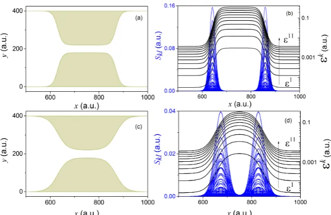
Figure 1.Two different nanojunctions, viz., (a) and (c), defined by EquationA17in AppendixDand usingA=180,B=220,a1=630,a2=870, withγ=10 in (a) andγ=20 in (c). Panels (b) and (d) show the associated second order (non-adiabatic) couplingsSkl_{(solid blue lines) and the associated} potential-energiesEk_{(x)(solid black lines) for the geometries in (a) and (c) respectively. Note that, due} to the symmetry of the states defined in Equation16, the coupling between odd and even states is zero, i.e.,Fkl(x) =Skl(x) =0, ∀k+l=odd.

The associated eigenvalues are given by:

Ek(x) = k 2_π2

2L2_(x), (17)

where we have defined L(x) = L1(x)−L2(x). These energies, parametrically dependent on the longitudinal variablex, define the effective potential-energies where the coefficientsχk(x,t)evolve on.

To evaluate the first and second order coupling termsFkl(x)andSkl(x), we need to rely on a particular form of the constriction. Depending on the specific form of L1(x)and L2(x), different geometrically bounded constrictions can be conceived (see for example the panels (a) and (c) of Figure1). Given the states in Equation 16and a particular shape of the constriction (defined in EquationA17of AppendixD), it is then easy to evaluate the non-adiabatic coupling termsFklandSkl (see panels (b) and (d) of Figure1).

The two different constrictions in Figure1serve well to gain some insight into the general form and dependence of the effective potential-energiesEk_{(x)as well as of the GNACs in Equation10.} Geometries changing more abruptly lead to sharper effective potential-energiesEk_{(x)and more peaked} non-adiabatic coupling termsFkl(x)andSkl(x). Sharper constrictions are thus expected to cause larger non-adiabatic transitions and hence to involve a larger number of transverse eigenstates requiring a larger number of longitudinal coefficients in order to reconstruct the reduced (longitudinal) density in Equation12. On the contrary, smoother constrictions should yield softer non-adiabatic transitions and hence involve a smaller number of transverse eigenstates and equivalently a smaller number of longitudinal coefficients.

3.2. Time-dependent propagation of the longitudinal coefficients

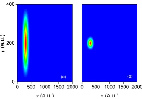
Figure 2. Panels (a) and (b) represent the probability density |Ψ(x,y, 0)|2_{, associated to the}

wavefunctions in Equations19and20respectively. Red regions in the plots correspond to higher probability densities while blue regions correspond to lower probabilities.

AppendixDusing the particular set of parameters,{A,B,a1,a2,γ}={180, 220, 630, 870, 20}, which

corresponds to panel (c) of Figure1. For this particular set of parameters, the symmetry of the states defined in Equation16forbids transitions between odd and even states, i.e.,

Fkl(x) =Skl(x) =0 ∀k+l=odd. (18) We will consider two different initial states. On one hand, the initial wavefunctionΨ(x,y, 0)will be described by:

Ψ(x,y, 0) =φ1_x(y)ψ(x), (19)

where φ1x(y) is the transverse ground state defined in Equation 16, and ψ(x) = Nexp

ik0(x− x0)exp−(x−x0)2

2σ2x

is a minimum uncertainty (Gaussian) wavepacket with initial momentum and dispersionk0=0.086 a.u. andσx=80 a.u. respectively, and centered atx0=300 a.u. (whileN is a normalization constant). On the other hand, we will consider the initial state to be defined by:

Ψ(x,y, 0) =ξ(y)ψ(x), (20)

where now bothξ(y)andψ(x) (defined above) are Gaussian wavepackets. In particular,ξ(y) =

Mexp−(y−y0)2 2σ2

withy0=200 a.u.,σy=20 a.u. (andMa normalization constant). The probability densities|Ψ(x,y, 0)|2_{associated to the above two initial states can be seen, respectively, in panels (a)} and (b) of Fig.2. Given the initial states in Equation19and Equation20, we can then deduce the corresponding longitudinal coefficients as follows:

χk(x, 0) =

Z

dyφk_x(y)Ψ(x,y, 0). (21)

While the initial state in Equation19corresponds to χk(x, 0) = δk1ψ(x), the state in Equation 20

involves a larger number of transverse eigenstates. Note that this second initial condition may be more realistic in practical situations, as large enough reservoirs may imply a quasi-continuum of transverse states according to Equation17.

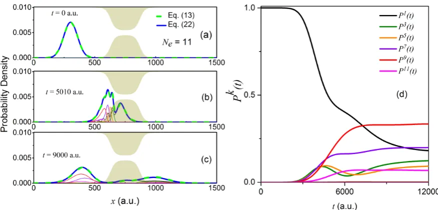
Figure 3.Time-evolution of the initial wavefunction in Equation19. The reduced density in Equation13

(dashed green line) as well as the reduced density in Equation22forNe=11 (solid dark blue) are shown at timest=300 a.u,t=5010 a.u. andt=9000 a.u in panels (a), (b) and (c) respectively. The rest of lines correspond to the absolute squared value of the longitudinal coefficients|χk(x,t)|. The evolution of the adiabatic populations in Equation23can be found in panel (d), using the same color code as in panels (a), (b) and (c).

evaluated from the full 2D wavefunction (dashed green line), as well as the reduced densityρ(x,t)

evaluated using the GC-TDSE scheme for a finite number of transversal statesNe, i.e:

ρ(x,t) =

Ne

∑

k=1

|χk(x,t)|2. (22)

In addition, we also show the absolute squared value of the longitudinal coefficients, i.e.,|χk(x,t)|2,

evaluated using the GC-TDSE. Alternatively, in the right panels of Figs.3and4we plot the population of each transverse state,

Pk(t) = Z

dx|χk(x,t)|2, (23)

as a function of time using the GC-TDSE.

The initial state in Equation19yieldsPk(0) =δk1. This can be seen in the right hand panel of Fig.3. This value stays constant until the wavepacket hits the constriction at aroundt=2500 a.u. At this moment, non-adiabatic transitions between different transverse states start to occur and lead to complicated interference patterns at later times (see, e.g., the reduced densityρ(x,t)att=5010 a.u.).

The number of significantly populated transverse states increases up to six (while up to eleven states are required to reproduce the exact reduced density up to a 0.1% error). Among these states, only odd transverse states are accessible due to the symmetry of the initial state (as we noted in Equation18). Since the mean energy of the initial state in Equation 19 (hE iˆ = 0.0037 a.u.) is higher than the barrier height of the first effective potential-energy in Figure1(d) (max(E1

x) =0.0028 a.u.), one could naively expect a complete transmission of the wavepacketχ1(x,t). However, due to the effect of the

non-adiabatic coupling termsFkl(x)andSkl(x),χ1(x,t)looses a major part of its population in favour

of higher energy transverse components that are reflected by much higher effective potential-energy barriers.

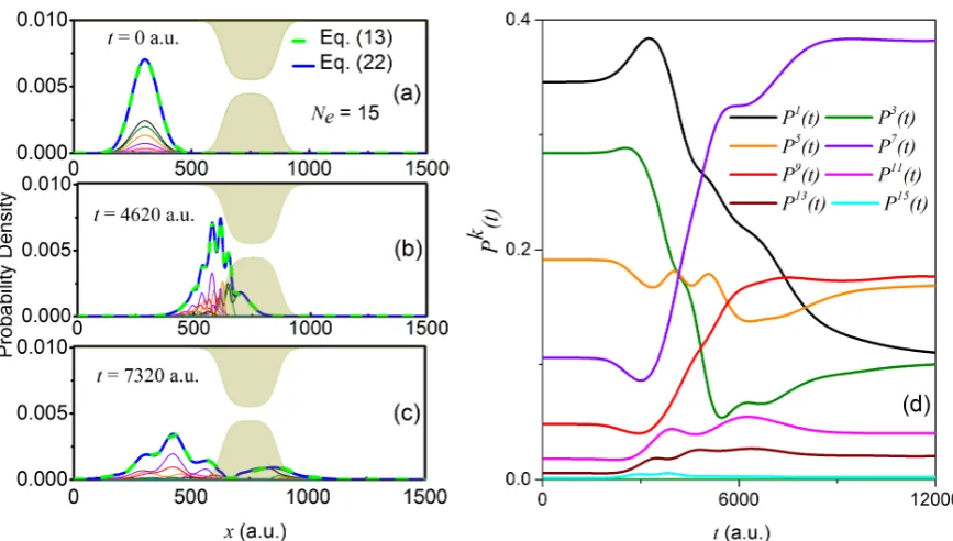
Figure 4.Time-evolution of the initial wavefunction in Equation20. The reduced density in Equation13

(dashed green line) as well as the reduced density in Equation22forNe=15 (solid dark blue line) are shown at timest =0 a.u,t=4620 a.u. andt=7320 a.u in panels (a), (b) and (c) respectively. The rest of lines correspond to the absolute squared value of the longitudinal coefficients|χk(x,t)|. The evolution of the adiabatic populations in Equation23can be found in panel (d), using the same color code as in panels (a), (b) and (c).

9 become more dominant than the previously dominant states 1, 3, and 5. Overall, up to 15 states become important to reproduce the exact reduced longitudinal density within a 0.1% error. Given the above two examples, it seems clear that the specific form of the impinging wavefunction does not play a determinant role in the scaling of the number of relevant transverse states even though it do effect the total number of statesNerequired to numerically evaluate Equation9.

Let us finally consider the effect that an external bias along the longitudinal direction might have on the numberNe of transverse eigenstates required to reproduce the solution of the full 2D TDSE. For that, starting with the state in Equation20, we consider the transmission coefficientT = R∞

−∞dy

R∞

xmdx|Ψ(x,y,tf)|

2_{for different values of the external potentialV}

ext = V(x)in Equation15. Written in terms of the Born-Huang expansion in Equation6, the transmission coefficientTreads:

T= Ne

∑

k=1

Z ∞

xm

dx|χk(x,tf)|2, (24)

wherexmis the center of the nanojunction in the longitudinal direction (i.e., with numerical value 750 a.u.) and tf is the time at which no probability density (i.e., less than 0.1%) remains inside the constriction. In Figure5we show results for applied bias 0.0075 a.u. ≤ Vext ≤ 0.045 a.u. and two different number of states Ne = 15 and Ne = 25. As expected, higher applied bias lead to a more vigorous collision of the wavepacket against the constriction due to a higher longitudinal momentum/energy, which allows higher energy transverse states to be populated.

4. General discussion

Figure 5.Figure depicting the transmission coefficient,T, under different bias voltages. This plot gives a comparison ofTbetween the exact 2D simulation (shown in dashed green line) and between the 1D simulation (shown in solid red line forNe=15 states and in solid blue line forNe=25 states). For a voltage range of 0.0075 a.u.≤Vext≤0.045 a.u.,Ne=25 states are enough to capture the exact 2D case. For max[Vext] =0.027 a.u.Ne=15 states sufficiently capture the exact 2D case.

functions. For a time-independent transverse Hamiltonian, the quantitiesEk_(x),Fkl_(x)andSkl_(x)are computed only once before the propagation of the longitudinal coefficients and thus the computational cost of the GC-TDSE resides, mainly, on the propagation of the 1D longitudinal coefficients.

Let us provide some numbers to get an estimate of the numerical efficiency of the GC-TDSE algorithm. Consider the numerical solution of the full 2D TDSE in a grid. For a number of grid points {nx,ny}={1500, 400}, the resulting Hamiltonian has a dimension(nx×ny)2. Alternatively, the size of the Hamiltonian involved in the propagation of the longitudinal coefficients of the GC-TDSE algorithm is(nx×Ne)2, whereNeis the number of transverse eigenstates. One can then estimate the numerical efficiency of one method over the other by simply evaluating the ratio(nx×ny)2/(nx×Ne)2. Thus, for time-independent transverse potentialsW(x,y,z), the computational reduction associated to the GC-TDSE isn2

y/Ne2. Note that the benefits of the GC-TDSE would be even more noticeable when applied to a 3D problem, for which the above ratio would become(n2y×n2z)/Ne2.

As we have seen in the above section, the number of required transverse statesNeis a function of the abruptness/smoothness of the constriction, but also of the energy of the impinging wavepacket. Therefore the computational advantage of the GC-TDSE method over the full dimensional TDSE is clearly system-dependent. Slow wavepackets impinging upon smooth constrictions would maximize the benefits of the GC-TDSE. Contrarily, very energetic electrons colliding against abrupt constrictions would certainly minimize its benefits. In this respect, we must note that the GNACs have a clear dependence upon the profile of the constriction. In particular, the second order coupling termsSkl_(x) will be sharply peaked for very abrupt constrictions (see the important differences in the size and sharpness of theSkl(x)in Figure1for two different constrictions). Therefore, due to the non-unitary character of the equations of motion of the longitudinal coefficients, very abrupt constrictions may demand very fine grids in practice.

not so obvious. As we have already noticed, for a time-dependent transverse potentialW(x,y,z,t), the eigenvalue problem in Equation5must be solved self-consistently with Equation9, i.e, at each time step. Then, a comparison of the GC-TDSE and the full dimensional TDSE in terms of numerical efficiency will depend on the specific performance of the eigensolver utilized to evaluate the transverse eigenvalues,Ek_{(x,t), and eigenstates}

φkx(y,z). 5. Conclusions

In this work we have proposed a new method, named GC-TDSE, that allows to include arbitrary geometric correlations between traversal and longitudinal degrees of freedom into a coupled set of 1D TDSE. Our motivation for the development of this method was, initially, a further reduction of the dimensionality of the 3D Schrödinger-like equations that result from a (Monte Carlo) SSE approach to quantum electron transport in open systems (valid for Markovian and non-Markovian regimes) that we have recently proposed [32]. Nevertheless, the method presented here is general and allows to reduce the dimensionality of quantum systems with geometrical correlations among different degrees of freedom, which could be of great utility in different research fields.

For smooth time-independent constriction profiles under low applied bias, our GC-TDSE method implies up to three orders of magnitude less computational resources than solving the full 3D TDSE directly. For very high applied bias or time-dependent constrictions profiles, the GC-TDSE may still be significantly cheaper than the solution of the full 3D TDSE, but would require introducing approximations to the solution of the potential-energiesEk_{(x,t)and the GNACs (F}kl_(x,t)andSkl_(x,t)). We thus expect the GC-TDSE presented here to trigger future investigation for making it robust against more extreme electron transport conditions and to inspire new ways of looking at the many-body problem.

Author Contributions: Conceptualization, D.P., X.O. and G.A. ; methodology, D.P., X.O. and G.A.; software, D.P.and G.A.; validation, D.P., G.A.and X.O.; formal analysis, D.P., X.O. and G.A.; investigation, D.P., X.O. and G.A.; resources, D.P., X.O. and G.A.; data curation, D.P., G.A., and X.O.; writing–original draft preparation, D.P., X.O. and G.A.; writing–review and editing, D.P., X.O. and G.A.; visualization, D.P., X.O. and G.A.; supervision, X.O. and G.A.; project administration, X.O. and G.A.; funding acquisition, X.O.

Funding:We acknowledge financial support from Spain’s Ministerio de Ciencia, Innovación y Universidades under Grant No. RTI2018-097876-B-C21 (MCIU/AEI/FEDER, UE). the European Union’s Horizon 2020 research and innovation programme under grant agreement No Graphene Core2 785219 and under the Marie Skodowska-Curie grant agreement No 765426 (TeraApps). G.A. also acknowledges financial support from the European Unions Horizon 2020 research and innovation programme under the Marie Skodowska-Curie Grant Agreement No. 752822, the Spanish Ministerio de Economa y Competitividad (Project No. CTQ2016-76423-P), and the Generalitat de Catalunya (Project No. 2017 SGR 348).

Conflicts of Interest:The authors declare no conflict of interest.

Appendix A Derivation of Equation9

In order to derive Equation9we start by introducing the expansion in Equation6into Equation1 to get:

i∂

∂t

∑

k_(x,t)

φk_x(y,z) =Tx

∑

χk(x)φk_x(y,z) +H(y,z)

∑

k

χk(x)φk_x(y,z) +V(x)

∑

k

χk(x)φk_x(y,z). (A1)

Making use of Equation5the above equation can be written as:

i∂

∂t

∑

k_(x,t)

φk_x(y,z) =Tx

∑

χk(x)φk_x(y,z) +Ek(x)

∑

k

χk(x)φk_x(y,z) +V(x)

∑

k

Expanding the termTx∑kχk(x)φkx(y,z)as:

Tx

∑

χk(x,t)φk_x(y,z) =

∑

k

(Txχk(x,t))φk_x(y,z)−1

2χ

k_(x,t) ∂2

∂x2φ

k

x(y,z)−

∂ ∂xχ

k_(x,t) ∂

∂xφ

k x(y,z)

,

(A3) and introducing it back into EquationA2one gets:

i∂

∂t

∑

k_(x,t)

φkx(y,z) =

∑

h

Tx+Ek(x)(y,z) +V(x) i

χk(x,t))φkx(y,z)

− 1 2

∑

χk(x,t) ∂

2

∂x2φ

k

x(y,z) +2

∂ ∂xχ

k_(x,t) ∂

∂xφ

k x(y,z)

(A4)

Multiplying both sides of EquationA4byR

dyR

dzφ∗_xl(y,z)and using the orthogonality condition,

R

dyR dzφ_x∗l(y,z)φk_x(y,z) =δk,lwe finally obtain:

i ∂

∂tχ

k_{(x,t) =}

Tx+Ek(x) +V(x)

χk(x,t)−

∞

∑

l=1

Skl(x) +Fkl(x) ∂

∂x

χl(x,t), (A5)

where we have definedSkl= 1₂R dyR dzφ∗_xl(y,z)∂2

∂x2φkx(y,z)andFkl= R

dyR dzφ∗_xl(y,z)_∂∂_xφk_x(y,z)as

the first and second order coupling terms respectively.

Appendix B Derivation of Equation11

Let us define the wavefunctions|φ_liand|φ_ki. Now evaluate the derivative of their inner product

as follows,

hφl|φki0=hφ_l0|φki+hφl|φ_k0i=δl.k=0, k6=l (A6) This implies,

hφ_l0|φki=−hφl|φ0_ki (A7)

Evaluating the expression given below,

hφl|H⊥|φki0 =hφ0_l|H⊥|φki+hφl|(H⊥)0|φki+hφl|H⊥|φ0_ki (A8)

where we have used the chain rule of differentiation. Using the eigenstate-eigenvalue relation from Equation5we get,

hφl|Hx⊥|φki0 =Ekhφ_l0|φki+hφl|(H⊥)0|φki+Elhφl|φ_k0i (A9)

Using the relation in EquationA7in EquationA9we get,

hφl|H⊥|φki0 = (El− Ek)hφl|φ0_ki+hφl|(H⊥)0|φki=0 (A10) In the above equation we have made use of the fact thathφ_l|H⊥|φ_ki0= (Ekhφ_l|φ_ki)0=0, whenk6=l

Therefore,

Fkl=hφl|(φki)0 =

hφl|(H⊥)0|φki

Which can be written in the position representation and using the same nomenclature as used in the main text as follows,

Fkl(x) = Z

dy

Z

dzφ∗_xl(y,z) ∂ ∂xφ

k

x(y,z) = R

dyR

dzφ_x∗l(y,z)

∂ ∂xH

⊥ x(y,z)

φk_x(y,z)

El_{(x)− E}k_(x) (A12) Using Equation4it is easy to see that only the potential functionW(x,y,z)will survive after the partial derivative with respect to the variablex. so we can equivalently write EquationA12as,

Fkl(x) = R

dyR

dzφ∗_xl(y,z)

∂

∂xW(x,y,z)

φ_k(y,z)

El_{(x)− E}k_(x) (A13) Appendix C Mean energy in a Born-Huang-like basis

The mean energy of a 3D system with a HamiltonianH(x,y,z)is given by, hE iˆ =

Z Z Z

dxdydzΨ∗(x,y,z)H(x,y,z)Ψ(x,y,z), (A14) which in terms of the Hamiltonian in Equation3and the wavefunction expansion in Equation6can be written as:

hE iˆ = ∞

∑

k,l Z

dxχ∗k(x,t)

Z

dy

Z

dzφ∗_xk(y,z)(Tx+V(x))φ_xl(y,z)χl(x,t)

+ ∞

∑

k,l Z

dxχ∗k(x,t)

Z

dy

Z

dzφ∗xk(y,z)H(y,z)φlx(y,z)χl(x,t). (A15)

Introducingn now Equation5and EquationA2into EquationA15we finally get:

hE iˆ = ∞

∑

k,l Z

dxχ∗k(x,t)

Z

dy

Z

dzφ∗_xk(y,z)

Txχl(x,t)φl_x(y,z)−1

2χ

l_(x,t) ∂2

∂x2φ

l x(y,z) − ∂

∂xχ

l_(x,t) ∂

∂xφ

l

x(y,z) +V(x)χl(x,t)φlx(y,z)

+

∑

Z

dxχ∗k(x,t)Exk(y,z)χk(x,t)

= ∞

∑

k Z

dxχ∗k(x,t)Txχk(x,t) +

∑

k Z

dxχ∗k(x,t)Exk(y,z)χk(x,t) +

∞

∑

k Z

dxχ∗k(x,t)V(x)χk(x,t)

+ ∞

∑

k,l

−1 2χ

∗k_(x,t)Z _dyZ _dz

φ∗_xk(y,z) ∂

2

∂x2φ

l x(y,z) − χ∗k(x,t)

Z

dy

Z

dzφ∗_xk(y,z) ∂ ∂xφ

l x(y,z)

∂ ∂x

χl(x,t)

= ∞

∑

k Z

dxχ∗k(x,t)

(Tx+Ek(x)(y,z) +V(x))χk(x,t) +

∞

∑

dzφ∗_xk(y,z) ∂

2

∂x2φ

l x(y,z) −

Z

dy

Z

dzφ∗xk(y,z)

∂ ∂xφ

l x(y,z)

∂ ∂x

χl(x,t)

= ∞

∑

k=1

Z

dxχ∗k(x,t)

"

Tx+Ek(x) +V(x)

χk(x,t)−

∞

∑

l=1

Skl(x) +Fkl(x) ∂

∂x

χl(x,t)

#

Appendix D Function defining the nano-constriction

For our numerical simulations in Section3we considered a prototypical constriction whereL1(x) andL2(x)in Equation14are defined as:

L1(x) =A "

1+expx−a1

γ

−1

+

1+exp−x+a2

γ

−1

#

+B, (A17a)

L2(x) =A "

1+exp−x+a1

γ

−1

+

1+expx−a2

γ

−1

#

− A, (A17b)

whereγdefines the sharpness of the constriction,AandBdefine the maximum and the minimum

width of the constriction, respectively max[L(x)] = B+A and min[L(x)] = B − A, anda1anda2 define the length of the constrictionLc=a2−a1.

1. Sharvin, Y.V. On the possible method for studying fermi surfaces. Zh. Eksperim. i Teor. Fiz.1965,48. 2. Jin, Z.; Li, X.; Zhou, W.; Han, Z.; Zhang, Y.; Li, Y. Direct growth of carbon nanotube junctions by a two-step

chemical vapor deposition. Chemical Physics Letters2006,432, 177–183.

3. Terrones, M.; Banhart, F.; Grobert, N.; Charlier, J.C.; Terrones, H.; Ajayan, P. Molecular junctions by joining single-walled carbon nanotubes.Physical review letters2002,89, 075505.

4. Peng, Y.; Cullis, T.; Inkson, B. Bottom-up nanoconstruction by the welding of individual metallic nanoobjects using nanoscale solder. Nano Letters2009,9, 91–96.

5. Shen, G.; Lu, Y.; Shen, L.; Zhang, Y.; Guo, S. Nondestructively Creating Nanojunctions by Combined-Dynamic-Mode Dip-Pen Nanolithography.ChemPhysChem2009,10, 2226–2229.

6. Takahashi, Y.; Nagase, M.; Namatsu, H.; Kurihara, K.; Iwdate, K.; Nakajima, Y.; Horiguchi, S.; Murase, K.; Tabe, M. Fabrication technique for Si single-electron transistor operating at room temperature. Electronics Letters1995,31, 136–137.

7. Maeda, K.; Okabayashi, N.; Kano, S.; Takeshita, S.; Tanaka, D.; Sakamoto, M.; Teranishi, T.; Majima, Y. Logic operations of chemically assembled single-electron transistor.ACS nano2012,6, 2798–2803. 8. Tans, S.J.; Verschueren, A.R.; Dekker, C. Room-temperature transistor based on a single carbon nanotube.

Nature1998,393, 49–52.

9. Zhang, L.; Zaric, S.; Tu, X.; Wang, X.; Zhao, W.; Dai, H. Assessment of chemically separated carbon nanotubes for nanoelectronics.Journal of the American Chemical Society2008,130, 2686–2691.

10. Nah, J.; Liu, E.S.; Varahramyan, K.M.; Tutuc, E. Ge-SxGe1−xCore–Shell Nanowire Tunneling Field-Effect Transistors. IEEE transactions on electron devices2010,57, 1883–1888.

11. Hu, Y.; Churchill, H.O.; Reilly, D.J.; Xiang, J.; Lieber, C.M.; Marcus, C.M. A Ge/Si heterostructure nanowire-based double quantum dot with integrated charge sensor. Nature nanotechnology2007,2, 622–625. 12. http://cobweb.ecn.purdue.edu/gekco/nemo3D/.

13. http://www.nextnano.de. 14. http://www.tibercad.org.

15. http://vides.nanotcad.com/vides/.

16. http://vonbiber.iet.unipi.it/Transiestatutorial/transiesta.html.

17. Jacoboni, C.; Reggiani, L. The Monte Carlo method for the solution of charge transport in semiconductors with applications to covalent materials. Reviews of modern Physics1983,55, 645.

18. Albareda, G.; Jiménez, D.; Oriols, X. Intrinsic noise in aggressively scaled field-effect transistors.Journal of Statistical Mechanics: Theory and Experiment2009,2009, P01044. doi:10.1088/1742-5468/2009/01/p01044. 19. Breuer, H.P.; Petruccione, F.; others.The theory of open quantum systems; Oxford University Press on Demand,

2002.

21. De Vega, I.; Alonso, D. Dynamics of non-Markovian open quantum systems. Reviews of Modern Physics

2017,89, 015001.

22. Vacchini, B. Non-Markovian dynamics for bipartite systems. Phys. Rev. A 2008, 78, 022112. doi:10.1103/PhysRevA.78.022112.

23. Gisin, N. Stochastic quantum dynamics and relativity. Helv. Phys. Acta1989,62, 363–371.

24. Pearle, P. Combining stochastic dynamical state-vector reduction with spontaneous localization.Physical Review A1989,39, 2277.

25. Carmichael, H.An open systems approach to quantum optics: lectures presented at the Université Libre de Bruxelles, October 28 to November 4, 1991; Vol. 18, Springer Science & Business Media, 2009.

26. Van Kampen, N.G.Stochastic processes in physics and chemistry; Vol. 1, Elsevier, 1992.

27. De Vega, I. Non-Markovian stochastic Schrödinger description of transport in quantum networks.Journal of Physics B: Atomic, Molecular and Optical Physics2011,44, 245501.

28. Goetsch, P.; Graham, R. Linear stochastic wave equations for continuously measured quantum systems.

Physical review A1994,50, 5242.

29. Gatarek, D.; Gisin, N. Continuous quantum jumps and infinite-dimensional stochastic equations. Journal of mathematical physics1991,32, 2152–2157.

30. Gambetta, J.; Wiseman, H. Non-Markovian stochastic Schrödinger equations: Generalization to real-valued noise using quantum-measurement theory. Physical Review A2002,66, 012108.

31. Rivas, A.; Huelga, S.F.; Plenio, M.B. Quantum non-Markovianity: characterization, quantification and detection. Reports on Progress in Physics2014,77, 094001.

32. Pandey, D.; Colomés, E.; Albareda, G.; Oriols, X. Stochastic Schrödinger Equations and Conditional States: A General Non-Markovian Quantum Electron Transport Simulator for THz Electronics.Entropy2019,21. doi:10.3390/e21121148.

33. Oriols, X. Quantum-Trajectory Approach to Time-Dependent Transport in Mesoscopic Systems with Electron-Electron Interactions. Phys. Rev. Lett.2007,98, 066803. doi:10.1103/PhysRevLett.98.066803. 34. Albareda, G.; Suñé, J.; Oriols, X. Many-particle hamiltonian for open systems with full coulomb interaction:

Application to classical and quantum time-dependent simulations of nanoscale electron devices.Physical Review B2009,79, 075315.

35. Colomés, E.; Zhan, Z.; Marian, D.; Oriols, X. Quantum dissipation with conditional wave functions: Application to the realistic simulation of nanoscale electron devices.Physical Review B2017,96, 075135. 36. Albareda, G.; López, H.; Cartoixa, X.; Suné, J.; Oriols, X. Time-dependent boundary conditions with

lead-sample Coulomb correlations: Application to classical and quantum nanoscale electron device simulators. Physical Review B2010,82, 085301.

37. Albareda, G.; Benali, A.; Oriols, X. Self-consistent time-dependent boundary conditions for static and dynamic simulations of small electron devices. Journal of Computational Electronics2013,12, 730–742. 38. Albareda, G.; Marian, D.; Benali, A.; Alarcón, A.; Moises, S.; Oriols, X., Electron Devices Simulation with

Bohmian Trajectories. InSimulation of Transport in Nanodevices; John Wiley and Sons, Ltd, 2016; chapter 7, pp. 261–318. doi:10.1002/9781118761793.ch7.

39. López, H.; Albareda, G.; Cartoixà, X.; Suñé, J.; Oriols, X. Boundary conditions with Pauli exclusion and charge neutrality: application to the Monte Carlo simulation of ballistic nanoscale devices. Journal of Computational Electronics2008,7, 213–216. doi:10.1007/s10825-008-0193-7.

40. Albareda, G.; Marian, D.; Benali, A.; Alarcón, A.; Moises, S.; Oriols, X. Electron devices simulation with Bohmian trajectories.Simulation of Transport in Nanodevices2016, pp. 261–318.

41. Born, M.; Huang, K.Dynamical theory of crystal lattices; Clarendon press, 1954.

42. Albareda, G.; Abedi, A.; Tavernelli, I.; Rubio, A. Universal steps in quantum dynamics with time-dependent potential-energy surfaces: Beyond the Born-Oppenheimer picture. Phys. Rev. A2016, 94, 062511. doi:10.1103/PhysRevA.94.062511.

43. González, L.; Lindh, R.Quantum Chemistry and Dynamics of Excited States: Methods and Applications; Wiley, 2020.