Virtual Force Based Sink Relocation Strategy in Wireless
Sensor Networks
Chengdong Wang
1, Xin Yang
1, Yong Feng
1*, Mingjing Tang
21 Yunnan Key Laboratory of Computer Technology Applications, Kunming University of Science and
Technology, Kunming, Yunnan 650500, China.
2 Key Laboratory of Educational Informatization for Nationalities, Ministry of Education, Yunnan Normal
University, Kunming, Yunnan 650500, China.
* Corresponding author. Email: [email protected]
Manuscript submitted June 20, 2018; accepted September 8, 2018. doi: 10.17706/ijcce.2018.7.4.107-118
Abstract: Sink relocation has been proven as an effective solution to relieve the network hot point problem, and to balance nodes’ energy consumption and thus prolong the network lifetime for wireless sensor networks. In this paper, we propose a Virtual Force based Sink Relocation strategy, called VFSR, which utilizes the resultant force derived from two kinds of virtual force, gravitational one and border repulsive one, to impel the sink node to relocate to the desired position. In VFSR, the gravitational force exists between each sensor and the sink, and is proportional to the node’s residual energy and inversely proportional to the distance from the node to the sink. The border repulsive force is adapted to avoid the sink node wandering nearby the network border. Under the action of the gravitational and the border repulsive force, the sink node approaches the nodes with high residual energy and makes them relay data from other nodes, which reduces data transmission overload of the nodes with low energy. Through simulation, we validate the effectiveness of VFSR.
Key words: Wireless sensor networks, network lifetime, sink relocation, virtual force.
1.
Introduction
In wireless sensor network (WSN), a large number of inexpensive sensor nodes (SNs) with limited battery energy are deployed in monitoring fields to sense the physical environments for a long period of time, even years [1], [2], and to forward sensed data back to one or more sink nodes through their wireless transceiver in a multi-hop manner. Such network deployment [3] implies the n-to-1 communication way in which the closer a sensor node is to the sink, the more data it undertakes to relay and thus the faster its battery runs out; whereas those further away from the sink only relay less packets or even nothing, thereby still maintain high residual energy [4]. This phenomenon is called the “energy-hole problem” [5], [6] or the “crowded center effect” [7], which degrade network performance, even split network, and shorten network lifetime [8].
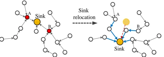
spots) are two hot spots for undertaking a lot of relaying. Before the two hot spots exhaust energy and result in the worse energy-hole, the sink moves to a new position, which can alleviate the hot spot situation of sensor A and B, and help to balance the energy consumption among all the sensors. But the cost is that a re-routing processing has to be launched. The new created forward paths are denoted as the blue line arrows. Therefore, efficient sink relocation schemes must make a good tradeoff between the improvement of the network performance and the increment of the topology management overhead resulting from sink moving.
Sink relocation Sink
Sink A
B
A
B
Fig. 1. Sketch of sink relocation in WSN.
To balance the energy consumption among all sensors while keeping low re-routing cost, many sink relocation schemes have been presented in recently years. According to the timing of making movement decision, the existing research work on the sink relocation can be broadly classified into two categories: the predetermined sink mobility path [10]-[13], [19], and autonomous sink movement [14]-[18]. The predetermined category schemes lack enough flexibility and scalability due to the moving path always has to be redesigned, so this paper takes autonomous sink movement.
In this paper, we introduce the virtual force concept into the sink relocation, and propose a new scheme VFSR in which the major contributions can be listed as follows:
We propose a new virtual force based sink relocation scheme VFSR, which uses the combined virtual force including both gravitational and border repulsive force to guide the sink to move.
We utilize the gravitational force to put nodes’ residual energy and the distance between the nodes and the sink together as a whole to consider. The gravitational force is used to drive the sink to move toward the sensors with high residual energy and high node density, which is beneficial for balancing the energy consumption among sensors.
We take use of the border repulsive force to avoid the sink wandering nearby the network’s border area, which is advantageous to improve the data gathering performance.
2.
The Background and Related Works
In [9], the authors explained the importance of sink relocating algorithm, and showed that the drawbacks found in multi-hop relaying can be overcome by sink relocating algorithm. In recent years, many sink relocation schemes have been proposed, which can be broadly classified into two categories: the predetermined sink mobility path and the autonomous sink movement.
time-sensitive applications, which aims to minimize this overhead while preserving the advantage of mobile sinks. First, ring nodes form a ring by greedy geographic routing algorithm, then sink moves along the ring and receives the data sent by the anchor nodes. Literature [19] proposes an Energy-Balanced Data Collection mechanism, called EBDC, which determines the trajectory of a mobile data collector (or mobile sink) such that the data-relaying workloads of all sensors can be totally balanced. In [13] author proposed sink node travel on a fixed trajectory in sensing area and collect the data from sensors and stored on the base station. The mobile sink node broadcast the predicated value to the sensor and only that sensor can send the data which exceeds the admissible error margin. However, a mobile sink that moves along some tracks or cableways lacks flexibility and scalability because its moving path always has to be redesigned when the sink is transplanted to other networks. And this category of relocation scheme dose not adapt to taking the current residual battery energy of sensor nodes into consideration, which will not be conducive to improve the network lifetime.
In contrast, autonomous moving strategies, in which a sink makes moving decisions according to the run-time circumstances, can provide reasonable adaptability to various types of network conditions. For example, Keontaek Lee et al. [14] establish a mixed integer linear programming model and a Greedy maximum residual energy algorithm(GMRE) based on the initial address of sink, route of data collection and dwell time. When the remaining energy of nodes around the neighbor’s location is larger than the current position, the sink will move to the neighbor node. In literature [15], an energy efficient and delay-aware path for mobile sink is proposed employing a heuristic method called WRP. However, this computation takes O(n5) time for n SNs. Mishra et al. [16] proposed an algorithm for designing a rendezvous point(RP)-based path for the mobile sink in delay-bound WSNs. In the proposed method, the target area is partitioned into hexagonal cells whose centers are considered as the potential positions of RPs. The mobile sink can aggregate the sensed data from all the sensors deployed in the network while visiting these RPs in its tour. However, the time complexity of this algorithm is high. Reference [17] proposes range constrained clustering (RCC). RCC divides nodes into several clusters and sink node stays at the cluster centers to gather data. The Concorde TSP solver is used to calculate the shortest movement path of sink node through some cluster centers. In the paper [18], lifetime optimization algorithm with mobile sink nodes for wireless sensor networks based on location information (LOA MSN) is proposed. Sink nodes gather the location information of sensor nodes and use the clustering method and graph theory method to find the movement paths. When the total transmission energy of node is greater than the threshold value and the overhead of moving sink is decided, then sink starts move to the new position.
3.
Virtual Force Base Sink Relocation Scheme Design
System Model
3.1.
create new routing paths, and then collect data messages from sensors.
System Working Process
3.2.
In this section, we will describe the system working process which includes three stages: routing building, data gathering, and relocation as follows.
(a) In routing building stage, the sink lies at some position in the network region. To communicate with sensors, the sink firstly broadcasts a routing building message to the sensors. With diffusing of the message, each sensor will obtain the routing path with the minimum hop number between it and the sink after a period of time.
(b) In data gathering stage, the sink collects data sensed by sensors through the routing paths set up in the routing building stage. Simultaneously, the sink also collects the residual energy information of sensors which can be piggybacked with data messages. The sink keeps checking whether the residual energy of one of its 1-hops neighbors is lower than a preset threshold 𝑅𝑡ℎ. Once the above condition is satisfied, the sink will switch to the next stage, i.e., relocation stage.
(c) In relocation stage, the sink will calculate its moving destination. For the sink knows all sensors’ position and can get its own position information timely, it can calculate the virtual gravitational force. Moreover, the sink also stores the information of the boundary region, thus it can know whether it lies in the boundary region, and calculate out the boundary repulsive force when it moves in the region. According to the method which will be presented in Section 3.3.3, the sink will determine its moving destination based on the total virtual exerted on it. After getting the moving destination, the sink checks whether the calculated destination is such a position where there is no any 1-hop neighbor, or where there is at least a 1-hop neighbor but the residual energy of one of the 1-hop neighbor(s) is lower than 𝑅𝑡ℎ. If so, the calculated position is invalid, and the sink will relocate a valid position where is at the segment connecting the sink’s current position and its calculated one and the nearest to the calculated position of the sink. The above three stages occur in sequence, and the network runs in such cyclical way.
Virtual Force Calculation
3.3.
The concept of virtual force is derived from physics, that is, when two atomic are close enough, they will be separated by the repulsive force, otherwise there will produce attractive force to draws them closer. Each atom moves according to the magnitude and direction of resultant force until it reaches equilibrium or the maximum value of movable distance. In [21], [22], virtual force is used to topology control, obstacle avoidance due to its intuition, easy description, and verifiability. We define the gravitational force between sink node and sensor node based on universal gravitation, and the boundary repulsive force based on Hooke's law. Therefore, each definition has the corresponding physical force to do support. The detailed calculation procedure of the two kinds of virtual force will be presented as follows.
3.3.1.
Virtual force calculation
According to the well-known universal gravitation formula between any two objects, i.e., 𝐹 = 𝐺𝑀𝑚𝑟2 , where M and m are the masses of the two objects respectively, and r is distance between them, and G is a constant, we can obtain the virtual gravitation between a sensor node i to sink node s , which is denoted as
𝐹𝑖
⃗⃗ .
𝐹𝑖
⃗⃗ = (𝑘𝐴𝑎𝑖
2𝑎2
𝑑𝑖𝑠2 , 𝛼𝑖𝑠) , 𝑖 ∈ 𝑁 (1)
is the Euclidean distance between i and s, and 𝛼𝑖𝑠 is the orientation (angle) to point from s to i, and 𝑎𝑖2, 𝑎2 is the residual energy of sensor i and the sink respectively. In order to highlight the major role what residual energy plays in the virtual gravitation, we use the square of the residual energy of a node to represent its mass. For the energy of the sink is regarded as being sufficient, it can be considered as a constant and be merged into 𝑘𝐴, then the Equation (1) can be simplified as:
𝐹𝑖
⃗⃗ = (𝑘𝐴𝑎𝑖
2
𝑑𝑖𝑠2, 𝛼𝑖𝑠) , 𝑖 ∈ 𝑁 (2)
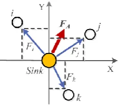
For there is a virtual gravitation between the sin and each sensor, the resultant force of which all nodes exerted on the sink s can be expressed as 𝐹⃗⃗⃗⃗ 𝐴 as follows:
𝐹𝐴
⃗⃗⃗⃗ = ∑ 𝐹𝑖 ⃗⃗ 𝑖, 𝑖 ∈ 𝑁 (3)
For example, considering there are three sensors i, j, k and the sink s in the monitoring area, as shown in Fig. 2 the resultant force ⃗⃗⃗⃗ 𝐹𝐴 exerted on the sink s can be expressed as ⃗⃗⃗⃗ = 𝐹𝐹𝐴 ⃗⃗ + 𝐹𝑖 ⃗⃗ + 𝐹𝑗 ⃗⃗⃗⃗ 𝑘. And the direction of the resultant force 𝐹⃗⃗⃗⃗ 𝐴 specifies the moving direction of the sink.
Fig. 2. Sketch of the virtual gravitational forces.
3.3.2.
Virtual force calculation
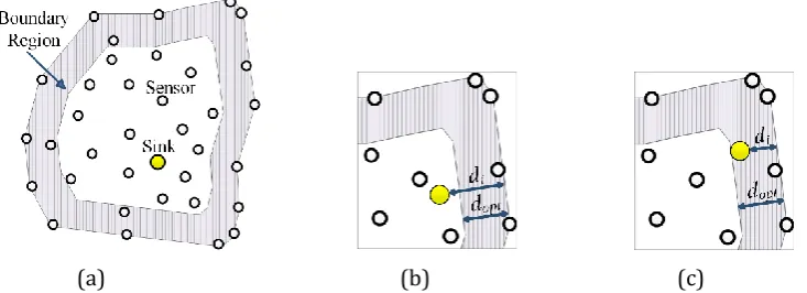
When the sink node moves autonomously under virtual gravity, the situation may appear in which the sink moves to the regional boundary and is far away from the vast majority of nodes. For virtual gravity is susceptible to distance, the gravitational forces exerted on the sink will be feeble which are derived from the nodes even if they are with higher residual energy but far from the sink. That may cause the sink wandering nearby the border and thus decrease the data gathering performance. To avoid the situation, we introduce the boundary repulsive force. Firstly, we define the distance threshold of area boundary as 𝑑𝑜𝑝𝑡, as shown in the Equation (4).
𝑑𝑜𝑝𝑡= {
𝛾, 𝐶𝑙𝑖𝑚(𝐴) < 1 𝛾
2, 𝐶𝑙𝑖𝑚(𝐴) ≥ 1
(4)
where 𝐶𝑙𝑖𝑚(𝐴) is the limit coverage [23], and when 𝐶𝑙𝑖𝑚< 1, the sensor node in the region is in a shortage state, 𝑑𝑜𝑝𝑡= 𝛾, and vice versa in a sufficient state, d𝑜𝑝𝑡= 𝛾/2 . Here, 𝛾 is the transmission radius of nodes.
acted on by the boundary repulsive force, and the closer the sink node is to the boundary, the greater the force it is. The above case is very similar to the compression spring in physics, therefore the boundary repulsive force is analogized with Hooke's law: 𝐹 = −𝑘𝑥 , in which 𝑥 is the length of the spring being deformed, and k is a constant. In the paper, the boundary repulsive force can be defined as:
𝐹𝑅
⃗⃗⃗⃗ = {(−𝑘𝑅𝑑⃗⃗⃗⃗⃗⃗⃗⃗⃗⃗⃗⃗⃗⃗⃗⃗⃗⃗ , 𝛼𝑖− 𝑑𝑜𝑝𝑡 𝑠+ 𝜋), 0 ≤ 𝑑𝑖< 𝑑𝑜𝑝𝑡
0, 𝐨𝐭𝐡𝐞𝐫
(5)
where 𝑑𝑖 is the distance between sink node and the boundary of region, and 𝑑⃗⃗⃗⃗⃗⃗⃗⃗⃗⃗⃗⃗⃗⃗⃗⃗⃗⃗ 𝑖− 𝑑𝑜𝑝𝑡 equivalent to 𝑥 .
𝑘𝑅 is the repulsion coefficient, its specific value will be given later in the experiment. And 𝛼𝑠 is the orientation (angle) of the vertical line from the sink node to the boundary, and 𝛼𝑠+ 𝜋 is the direction of the boundary repulsive force. In Fig. 3(b), when 𝑑𝑖≥ 𝑑𝑜𝑝𝑡, the sink is not in the boundary region and not affected by the boundary repulsive force. When 𝑑𝑖 ≤ 𝑑𝑜𝑝𝑡, the sink node will be acted on by the boundary repulsive force as shown in Fig. 3(c).
(a) (b) (c)
Fig. 3. Three kinds of relocate position between sink node and regional boundary. (a) Global network layout; (b) 𝑑𝑖≥ 𝑑𝑜𝑝𝑡; (c) 0 ≤ 𝑑𝑖≤ 𝑑𝑜𝑝𝑡.
3.3.3.
Total force exerted on the sink
From the discussion mentioned above, we know that the sink node may be acted on by two kinds of virtual forces: the gravity force and the boundary repulsive one. The gravity from all sensors is always there. But the boundary repulsive force exists only when the sink lies in the boundary region. Thus the total force exerted on the sink node s can be given by the following Equation:
𝐹(𝑠)
⃗⃗⃗⃗⃗⃗⃗⃗⃗ = {𝐹⃗⃗⃗⃗⃗⃗⃗⃗⃗⃗⃗ + 𝐹𝑅(𝑠) ⃗⃗⃗⃗⃗⃗⃗⃗⃗⃗ , 0 ≤ 𝑑𝐴(𝑠) 𝑖< 𝑑𝑜𝑝𝑡
𝐹𝐴(𝑠),
⃗⃗⃗⃗⃗⃗⃗⃗⃗⃗⃗ 𝑑𝑖≥ 𝑑𝑜𝑝𝑡
(6)
3.3.4.
Moving destination calculation for the sink
After getting the virtual force, the sink need to determine toward which direction and how long it will move based the direction and the magnitude of virtual force. When 𝐹(𝑠)⃗⃗⃗⃗⃗⃗⃗⃗⃗ is 0, the sink keeps stationary; when 𝐹(𝑠)⃗⃗⃗⃗⃗⃗⃗⃗⃗ is more than 0, the sink node starts to move guided by the resultant force, and the moving distance increases with the magnitude of the force increasing. The moving distance of the sink should be proportion to the 𝐹(𝑠)⃗⃗⃗⃗⃗⃗⃗⃗⃗ . Thus we use the Equation (7) to convert the virtual force into the moving distance of the sink node s:
where 𝛿 is a coefficient of proportionality, and the direction of sink node moving is consistent with the direction of virtual force. Based on the magnitude and direction of the virtual force, the new location
(𝑥relocate, 𝑦relocate) can be calculated as follows:
{
𝑥relocate= 𝑥current+|𝐹(𝑠)⃗⃗⃗⃗⃗⃗⃗⃗⃗ ||𝐹⃗⃗⃗⃗ |𝑥 ∗ 𝑑(𝑠)
𝑦relocate= 𝑦current+ |𝐹⃗⃗⃗⃗ |𝑦 |𝐹(𝑠) ⃗⃗⃗⃗⃗⃗⃗⃗⃗⃗ |∗ 𝑑(𝑠)
(8)
where 𝐹⃗⃗⃗ 𝑥 and 𝐹⃗⃗⃗ 𝑦 are the forces exerted on the sink in x and y direction respectively, and (𝑥current, 𝑦current) is the current location of the sink.
4.
Performance Evaluation
Simulation Setup
4.1.
In the section, we compared the performance of VFSR with that of two typical sink relocation strategies: EASR [20] and One-Step [25]. EASR is a kind of energy-aware relocation strategy, which utilizes the residual energy information of nodes to move the sink and dynamically change the transmission radius of sensors. One-step makes the moving destination of the sink only according to residual energy of sensor regardless of the distance between sink and sensor. The network lifetime is used the main measure of performance in this paper, which is defined as the period of time until the first sensor node dies. We define the transmission delay of data as the time interval between the time data is generated and the time it is transferred to the sink, so the delivery delay represents the average transmission delay of all nodes in each cycle. Here, we adopt the radio energy model of literature as energy consumption model. In this energy model, transmit and receive messages are the main consumption.
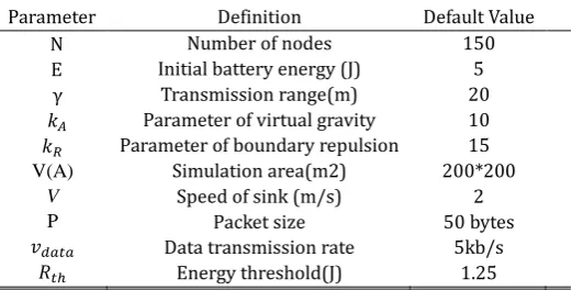
In order to investigate the performance of VFSR, we conducted simulation experiments in five different scenarios: the different value of 𝑅𝑡ℎ; the number of sensor nodes; the initial battery energy of nodes; the moving speed of sink node and the transmission range. The main simulation parameters are listed in Table 1.
Table 1. Parameter Setting of Simulation Environment
Parameter Definition Default Value
N E γ 𝑘𝐴 𝑘𝑅 V(A) V P 𝑣𝑑𝑎𝑡𝑎 𝑅𝑡ℎ
Number of nodes Initial battery energy (J)
Transmission range(m) Parameter of virtual gravity Parameter of boundary repulsion
Simulation area(m2) Speed of sink (m/s)
Packet size Data transmission rate
Energy threshold(J) 150 5 20 10 15 200*200 2 50 bytes 5kb/s 1.25
Experimental Results and Analysis
4.2.
4.2.1.
The value of energy threshold
𝑹
𝒕𝒉is too large, the frequent relocation of sink will result into high overhead of rerouting, which is also not conducive to save the energy consumption in the whole network. Therefore, the paper takes 𝑅𝑡ℎ′𝑠 value as 25% of initial energy.
Fig. 4. The influence of 𝑅𝑡ℎ on network performance.
4.2.2.
Performance under different node transmission range
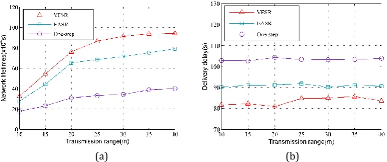
Fig. 5 shows the network performance comparison results of three sink node relocation strategies when the transmission range of sensor nodes changes. As show in Fig. 5(a), when the transmission range increases, the network lifetime of the three strategies increases as well. As the transmission range becomes larger, the length of the total transmission path (total hops of data transfer) will be reduced and the number of neighbors with respect to the sink will be increased, so that the overall network lifetime is improved. From Fig. 5(b) we can see that the average transmission delay of one-step is the highest and VFSR has the least delivery delay compared to other two strategies, so the sink node can collect and process data in a shorter period of time. In general, the performance of the VFSR is superior to the other two relocation strategies, because in VFSR, the sink is relocated to the nodes with more residual energy each time, so the neighbor nodes of sink can perform more relay tasks.
(a) (b)
Fig. 5. The influence of different transmission ranges of each node on network performance. (a) The influence on network lifetime; (b) The influence on average delivery delay.
4.2.3.
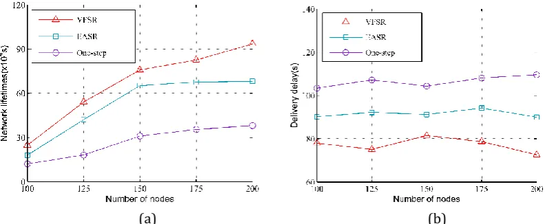
Performance under different node number
VFSR has the least delivery delay compared to other strategies, that is, the sink node can collect and process data in a shorter period of time. And the average transmission delay of one-step is the highest, perhaps it is because the sink moves to destination regardless of the distance, this leads to increased transmission delay for other nodes.
(a) (b)
Fig. 6. The influence of different node densities on network performance. (a) The influence on network lifetime; (b) The influence on average delivery delay.
4.2.4.
Performance under different sink speed
Fig. 7 shows change of the network lifetime and average delivery delay when the speed of sink node is changed and the performance of VFSR is much better than the other two strategies. In Fig. 7 (a), network lifetime of all curves is small when the speed of sink node is 0, this is because the sink is stationary at this time and will cause very serious energy-hole problems. When speed less than 0.5m/s, the curve of VFSR is increasing, but both of network lifetime and delivery delay are decreasing gradually when the speed is increasing. That is because the faster the speed of sink node, the more the number of relocation of sink increases and the more frequent data transmission is collected between other SNs, which leads to reduce the transmission delay of data, but at the same time, it speed up energy consumption and reduce the network lifetime. From Fig. 7(a) and (b) we can see that with the change of sink speed, the lifetime and transmission delay of one-step are not changed greatly. This is because sink regardless of distance and directly “jump” to Moving Destination, so the speed of sink has little effect on its algorithm.
(a) (b)
5.
Conclusions
In this paper, we proposed a new sink relocation strategy called VFSR to improve the network lifetime and performance. The proposed VFSR utilizes two categories virtual force, i.e., gravitational one and border repulsive one, and applies the combined effect of both the two force on the sink in order to impel it to relocate. The gravitational force makes the sink node approach the nodes with high residual energy, and the border repulsive force can avoid the sink node wandering nearby the network border. Simulation results show that the proposed VFSR can reach better performance compared with the existing typical sink relocation algorithms: One-Step and EASR, in terms of network life, and data delivery delay.
Acknowledgement
This work is supported by the National Natural Science Foundation of China under Grants no. 61662042, 61262081, and 61462053; the Yunnan Provincial Key Project of Applied Basic Research Plan under Grants no. 2014FA028.
References
[1] Grover, J., & Rani, R. (2014). Probabilistic density based adaptive clustering scheme to improve network survivability in WSN. Proceedings of the IEEE Fifth International Conference on Computing, Communications and Networking Technologies (pp. 1-7). Hefei, Anhui, China.
[2] Grover, J., Shikha, & Sharma, M. (2014). Location based protocols in wireless sensor network — A review. Proceedings of the International Conference on Computing, Communication and Networking Technologies (pp. 1-5). Hefei, Anhui, China.
[3] Tyagi, S., & Kumar, N. (2013). A systematic review on clustering and routing techniques based upon leach protocol for wireless sensor networks. J. Netw. Comput. Appl., 36, 623-645.
[4] Lian, J., Naik, K., & Agnew, G. B. (2006). Data capacity improvement of wireless sensor networks using non-uniform sensor distribution. Int. J. Distrib. Sens. Netw., 2, 121-145.
[5] Li, J. & Mohapatra, P. (2005). An analytical model for the energy hole problem in many-to-one sensor networks. Proceedings of theIEEE Vehicular Technology Conference (pp. 2721-2725). Dallas, Texas, USA. [6] Li, J. & Mohapatra, P. (2007). Analytical modeling and mitigation techniques for the energy hole
problem in sensor networks. Pervas. Mobile Comput., 3, 233-254.
[7] Popa, L., Rostamizadeh, A., Karp, R., Papadimitriou, C., & Stoica, I. (2007). Balancing traffic load in wireless networks with curveball routing. Proceedings of theACM International Symposium on Mobile Ad Hoc Networking and Computing, Montreal (pp. 170-179). QC, Canada.
[8] Zhang, P., Xiao, G., & Tan, H. P. (2013). Clustering algorithms for maximizing the lifetime of wireless sensor networks with energy-harvesting sensors. Comput. Netw., 57, 2689-2704.
[9] Shrivastava, P. B., & Pokle, S. (2012). Survey on sink repositioning techniques in wireless sensor networks. Int. J. Comput. Appl., 51, 9-20.
[10]Marta, M., & Cardei, M. (2009). Improved sensor network lifetime with multiple mobile sinks. Pervas. Mobile Comput., 5, 542-555.
[11]Wang, J., Cao, J., Cao, Y., Li, B., & Lee, S. (2015). An improved energy-efficient clustering algorithm based on MECA and PEGASIS for WSNS. Proceedings of the 2015 Third International Conference onAdvanced Cloud & Big Data (pp. 262-266).
[12]Tunca, C., Isik, S., Donmez, M. Y., & Ersoy, C. (2015). Ring routing: An energy-efficient routing protocol for wireless sensor networks with a mobile sink. IEEE Trans. Mobile Comput., 14, 1947-1960.
[14]Lee, K., Kim, Y. H., Kim, H. J., & Han, S. (2014). A myopic mobile sink migration strategy for maximizing lifetime of wireless sensor networks. Wirel. Netw., 20, 303-318.
[15]Salarian, H., Chin, K. W., & Naghdy, F. (2014). An energy-efficient mobile-sink path selection strategy for wireless sensor networks. IEEE Trans. Veh. Technol., 63, 2407-2419.
[16]Mishra, M., Nitesh, K. &, Jana, P. K. (2016). A delay-bound efficient path design algorithm for mobile sink in wireless sensor networks. Proceedings of the2016 3rd International Conference on Recent Advances in Information Technology (RAIT) (pp. 72-77). Dhanbad India.
[17]Kumar, A. K., Sivalingam, K. M., & Kumar, A. (2013). On reducing delay in mobile data collection based wireless sensor networks. Wirel. Netw., 19, 285-299.
[18]Chen, Y., Wang, Z., Ren, T., & Lv, H. (2015). Lifetime optimization algorithm with mobile sink nodes for wireless sensor networks based on location information. Int. J. Distrib. Sens. Netw., 2015, 1-11.
[19]Hui, L., Chai, Z. J., & Du, J. Z. (2011). Sensor redeployment algorithm based on combined virtual forces in three dimensional space. Acta Autom. Sin., 37, 713-723.
[20]Wang, C. F., Shih, J. D., Pan, B. H., & Wu, T. Y. (2014). A network lifetime enhancement method for sink relocation and its analysis in wireless sensor networks. IEEE Sens. J., 14, 1932-1943.
[21]Dang, X. C., Shen, S. C., Hao, Z. J., Zhao, H. Z., & Xu, Y. J. (2016). Mobile coverage algorithm based on virtual force in WSN. Comput. Engr. Appl., 52, 88-93.
[22]Wang, T., Sun, Y., Zhao, X. U., & Zhang, X. (2016). Coverage optimization algorithm based on virtual force for heterogeneous wireless sensor networks. Chin. J. Sens. Act., 8, 1253-1259.
[23]Li, X., Frey, H., Santoro, N., & Stojmenovic, I. (2008). Localized sensor self-deployment with coverage guarantee. ACM Sigmobile Mobile Computing & Communications Review, 12, 50-52.
[24]Chen, C. T., & Sun, Y. (2011). Efficient boundary detection algorithm of wireless sensor networks. Comput. Eng. Des., 32, 2984-2988.
[25]Bi, Y., Niu, J., Sun, L., & Wei, H. (2007). Moving schemes for mobile sinks in wireless sensor networks. Proceedings of the IEEE International Performance, Computing, and Communications Conference, IPCCC 2007 (pp. 101-108).
Chengdong Wang received the B.S. degree in computer science and technology from Suzhou University, China. He is currently a postgraduate student in the Yunnan Key Laboratory of Computer Technology Applications, Kunming University of Science and Technology, Kunming, Yunnan, China. His current research interest is wireless sensor network.
Yong Feng received the PhD degree in information and communication engineering from the University of Electronic Science and Technology of China in 2011. He is currently an associate professor at the Faculty of Information Engineering and Automation in the Kunming University of Science and Technology, China. His research interests mainly include mobile computing, ad hoc network, and distributed systems. He is a member of the IEEE.