www.astrophys-space-sci-trans.net/3/1/2007/ © Author(s) 2007. This work is licensed
under a Creative Commons License. Astrophysics and Space Sciences
Transactions
Predicting the future from observable sequences of events in
astrophysics I. Maximum Likelihood Estimation for a fixed number
of parameters
C. R¨oken and I. Lerche
Institut f¨ur Theoretische Physik, Lehrstuhl IV: Weltraum und Astrophysik, Ruhr-Universit¨at-Bochum, 44780 Bochum, Germany
Received: 8 November 2006 – Revised: 14 May 2007 – Accepted: 25 May 2007 – Published: 30 July 2007
Abstract. Using analytical and numerical methods, esti-mates are given of future predictions in astrophysics that can be gathered from a sequence of observed events, for exam-ple forγ-ray bursts. Some general probability considera-tions are provided and then a maximum likelihood estima-tion, together with an approximation for the large number limit of possible events. Illustrations are given of the numer-ical maximum likelihood estimation programs in the situa-tions of both a large number and a finite number of events. The effects of data uncertainty are also considered. Numer-ical calculations and comparisons with theoretNumer-ical expecta-tions are presented too.
1 Introduction
In many fields of astrophysics one can observe a sequence of events, each of different intensity. Perhaps such is best exemplified by observations ofγ-ray bursts which are short and intense pulses of softγ-rays, where short means that the pulses can last from a fraction of a second to several hundred seconds. All knownγ-ray bursts originate in extragalactic regions. Possible sources are for example core-collapsing rapidly rotating Wolf-Rayet stars or two colliding neutron stars orbiting in a binary. Today it is known that the form of aγ-ray burst is a narrow beam with corresponding en-ergies around 1051 ergs (Frail et al., 2001; Panaitescu and Kumar, 2001; Piran et al., 2001). γ-ray bursts are detected in random directions, so they are an isotropic phenomenon. For example seven γ-ray bursts with photon energies that lie in an interval of 100 MeV to 18 GeV were measured with the high energyγ-ray detector Gamma-Ray Experiment Telescope (EGRET) at the Compton Gamma-Ray Observa-tory (Dingus and Catelli, 1998). For more detailed infor-mation aboutγ-ray bursts useful references are Piran (1999,
Correspondence to: C. R¨oken ([email protected])
2000, 2004); Hurley (2002); Fishman and Meegan (1995); van Paradijs et al. (2000). Predictions of the energetics and the rate of such a sequence ofγ-ray bursts with different in-tensities can be statistically discussed as shown in this paper. One can formulate the questions of prediction in a more general way: From the observations of M events can one predict the most probable number, N, of all such observable events? Can one predict the fraction of all possible observ-able events that could lie less than (greater than) a given in-tensity? Can one predict whether the next event to arrive will lie above or below a given intensity? With what degree of confidence can one make any such predictions?
The purpose of this paper is to provide a set of procedures allowing one to address these questions under the following conditions:
1. Each event is statistically independent (no correlation) with any and all other events.
2. Each event arising from the remaining undiscovered population of events is random, with the probability of being measured proportional to a power of the arrival flux.
2 Technical development
2.1 Probability considerations
Consider an ordered sequence of observed events, with eventiof intensity Ii, and withM events measured. Sup-pose that a total of N events exists. One is interested in the probability that event M+1 will have an inten-sityIM+1 in excess of (or less than) a chosen value Icut, based on the information of the first M measured ordered events. For the N total events, let there be N1 character-ized by the average intensityF1 := PlowIi
/m1, where the sum P
low extends over those events with intensities less thanIcutandN2characterized by the average intensity F2 := PMi=1Ii−PlowIi/m2, with N1+N2=N and m1+m2=M. Note that this representation requires at least one observed event to lie aboveIcut. The probability that the first event lies in the class described byF1is
p1=
F1aN1 N1F1a+N2F2a
(1) wherea is the parameter of observability to be determined (see later) while the probability that the first event lies in the class described byF2is
p2=1−p1=
F2aN2 N1F1a+N2F2a
(2) After m1 measured events in class F1 and m2 measured events in classF2, the probability the next event is in class j (j=1,2)is
pnext(j )=
Fja Nj−mj
F1a(N1−m1)+F2a(N2−m2)
(3) Set the membership classkij=1 if theit hevent is in classj, andkij=0 if theit hevent is not in classj, withki1+ki2=1. Then, afterMevents, orderedi=1, ..., M, the joint proba-bility distribution is
p (M;N1, N2;a)= M
Y
i=1
P2
j=1kijFja Nj −Pit−=11ktj
P2
j=1Fja Nj−Pit−=11ktj
(4)
WithF1/F2=randN2=N−N1Eq. (4) can be written:
p (M;N, N1;a) (5)
= M
Y
i=1
ki1ra N1−Pti=−11kt1+ki2 N−N1−Pti−=11kt2
ra N
1−Pit−=11kt1
+N−N1−Pit−=11kt2
where the terms in the summations have to be omitted for i=1, the first event in the ordered sequence. Note that because only two classes are available (events with inten-sities below the cut and events with inteninten-sities above the cut) and because a given event must lie somewhere, then ki1=1−ki2. We use this fact in the next subsection. Un-known in Eq. (5) are the total numberNof events that can oc-cur,N1the number of events in the class characterized byF1,
as well as the parametera. There are at least two procedures available to provide estimates of the parametersN, N1anda based on theMmeasured events. The procedures are: Max-imum likelihood estimation and Bayesian updating (Aldrich, 1997; Fisher, 1925; Fisher , 1934; Arps et al., 1971; Jaynes, 1978).
In this paper we consider first the maximum likelihood es-timation in general and then discuss the situation when the number of observed events to date,M, is taken to be small compared to the number,N, of available events.
2.2 Maximum Likelihood Estimation
The joint probability distribution given by Eq. (5) comes as close as it can to matching the observed sequence of events when Eq. (5) takes on its maximum value with respect to the parametersN, N1 anda. It is convenient to change the variableN1toNsin2θwhenN2=Ncos2θand to then use N, cosθ (=µ)andaas basic variables. The joint probability distribution has extremum values when
∂p ∂N =0;
∂p ∂µ =0;
∂p
∂a =0. (6)
Note, however, that an extremum can be a maximum, mini-mum or point of inflection. Also note that the absence of an extremum does not imply the absence of a maximum. For instancep=µ2(0≤µ≤1)has no extremum in 0≤µ≤1, nevertheless it has a maximum atµ=1. Further, the param-etersN, µ2anda at an extremum can end up in physically unacceptable domains (e.g. N <0, µ2<0, µ2>1, a <0, etc.) in which case the extremum, even if a maximum, is not physically appropriate. We return to this point a little later.
From∂p/∂N=0 one obtains the constraint M
X
i=1
ki1ra+µ2(ki2−ki1ra) [N[ki1ra+µ2(ki2−ki1ra)] −αi]
= M
X
i=1
ra+µ2(1−ra) [N[ra+µ2(1−ra)] −β
i]
(7) where
αi =ki1ra i−1
X
t=1
kt1+ki2 i−1
X
t=1
kt2 (8)
and βi =ra
i−1
X
t=1 kt1+
i−1
X
t=1
kt2 (9)
withα1=β1=0.
From∂p/∂µ=0 one obtains the constraint M
X
i=1
ki2−ki1ra
N[ki1ra+µ2(ki2−ki1ra)] −αi = 1−ra
M
X
i=1
while from∂p/∂a=0 one obtains the constraint M
X
i=1
ki1
N[ki1ra+µ2(ki2−ki1ra)] −αi =
M
X
i=1
(N[ra+µ2 1−ra] −βi)−1 (11)
unlessr=1 in which case Eq. (11) is ignorable. Forr6=1 the three constraints are not independent because one can imme-diately derive the third constraint from any two of Eqs. (7), (10) and (11). Thus, at best one can derive two ofN, µanda as functions of the third parameter. The constraint equations do not admit of simple analytic solutions for, say,N andµ as functions ofafor a setM of observations, except in the somewhat simple case whenM=2.
Because a priori estimates forN andµare needed in the Bayesian update procedure (see Appendix A), it is conve-nient to develop here the estimates ofN andµfor the case M=2. Then
N (M=2)=r−a[A−(1−ra)B] (12)
µ2(M =2)= Br
a
A−(1−ra)B (13)
whereAandBsatisfy the pair of equations 2B(1−2k22)(1−2k11)
= −α1(1−2k11)
+A[(1−2k11)(1−k22)−k11(1−2k22)] (14) A(A−β1)(1−k11−k22)
=(1−2k22)(2A−β1[Ak11+(1−2k11)B] (15) Equations (14) and (15) provide linear algebraic equations for determiningAandB. Two requirements on the solution are
1. A > B(1−ra)andA >0; 2. A > B
in order that the estimates N (M=2) >0 and µ2(M=2) >0. If A > B and A >0 then A > B(1 −ra) for alla≥0 in r <1. Thus one only has to search for the solution of Eqs. (14) and (15) withA > BandA >0. From Eqs. (14) and (15) one has
A=β1α1(1−2k11)
·[2α1(1−2k11)+β(k11+k22−1)]−1 (16)
B = α1
1−2k22
[β1k11(2k22−1)−α1(1−2k11)] [β1(k11+k22−1)+2α1(1−2k11]
(17) For a given two event situation (where at least one event must have an intensity above Icut), it may happen that Eqs. (16) and (17) do not permit N (M=2) >0 and/or 0≤µ2(M=2)≤1 in which case the extremum constraints
do not represent a physically allowable maximum. The same sense of requirement of physical allowability is true for anyN (M), µ2(M)anda(M), not just forM=2. Thus, the constraint Eqs. (7) and (10) (which are impossible to solve analytically for M≥5) may not provide acceptable (N >0,0≤µ2≤1, a≥0)ranges for the desired parameters. One way to avoid this extremum problem is to ignore the extremum constraint approach and deal directly with Eq. (4) in the form
p (M;N;µ, a)
= M
Y
i=1
ki1ra Nsin2θ−γi
+ki2 Ncos2θ−δi
ra Nsin2θ−γ
i+Ncos2θ−δi
(18)
withγi=Pit−=11kt1andδi=Pit−=11kt2.
Monte Carlo searching ina≥0, N≥M,0≤µ2≤1 then enables one to determine rapidly the parameter values yield-ing the maximum probability. In this situation one uses the physical acceptability requirements first so that one is guar-anteed all values ofpwill lie in 0≤p≤1. One catch is that there is no guarantee that the three parametersN, µ2, awill be unique. It can happen that multiple domains in(N, µ2, a) space will all produce an identical maximum probability. Thus a broad search is then required in order to identify all such domains and determine how to proceed further to nar-row down, or eliminate, some of the domains.
One strategy that has proved somewhat successful in this regard is the so called Training Procedure (Lerche, 1997). Start withM=2 and ensure that at least one of the first two events has an intensity aboveIcut. Run Monte Carlo sim-ulations in N≥2,0≤µ2≤1, a >0 and record the largest value ofp(M=2), saypmax(2), and theN, µ2andavalues at whichpmax(2)occurs. In the event multiple domains in (N, µ2, a) space provide the same pmax(2)record all such domains. Now increase M from M=2 to M=3 and re-peat the Monte Carlo procedure, again identifying all do-mains wherepmax(3)occurs. Carry through this operational sequence at ever increasingMuntil all the observed events have been used. Then investigate the stability of the domains in (N, µ2, a) space to determine these regions that provide a neighborhood within which (N, µ2, a) stay and those do-mains that are highly unstable with respect to increases in M, i.e. these domains where (N, µ2, a) for pmax(M) de-part massively from the domains forpmax(M+1). Then it is highly unlikely that such unstable domains represent appro-priate values of the triad (N, µ2, a), although they can not be categorically ruled out. Check the value ofpmax(M)in relation to unity. Ifpmax(M)is close to unity then the pa-rameter triad obtained represents the statement that the max-imum likelihood estimation is close to the observed sequence (Cronquist, 1991).
much ad hoc user evaluation in the sense of being required to assess stable and unstable domains asM is increased. Sec-ond, the strategy requires a qualitative judgement on what constitutes close to unity forpmax(M). Third, the strategy is hardly unassailable as a procedure that will provide sys-tematic improvements as the number of observed events is increased. Fourth, the strategy is extremely ineffective in as-sessing the number,N, of possible observable events when NMas we show in the next section of the paper. A better, and systematic, method is required for steady improvement as one increases the number of ordered observed events from M=2 to the total observed,M. Precisely that concern is ad-dressed by Bayesian updating. We discuss the Bayesian pro-cedure in a later paper. However, the basic mathematical de-velopment for the Bayesian procedure is given in Appendix A. Equally, a systematic automatic procedure for assessing the relevant ranges of parameters is given in Appendix B (Lerche, 1997; Lumley, 1970).
Those mathematical developments are presented here both for the sake of completeness as well as so that only numerical procedures and their implementation and applications need be given in the second paper of this series.
2.3 The limit of large number of possible events,NM Expansion of Eq. (18) for NM yields, to first order in 1/N, that
p=
(M Y
i=1
[ki1rasin2θ+ki2cos2θ] rasin2θ+cos2θ
)
×
(
1−r a N
M
X
i=1 ·[γicos
2θ (k
i1ra−ki2)+δisin2θ (ki2−ki1)] ki1rasin2θ+ki2cos2θ cos2θ+rasin2θ
)
(19)
If one were to ignore the term factored by 1/N in Eq. (19) then the probability distribution is independent ofN, indicat-ing that one could perform a lowest order Monte Carlo search for the values ofµ2andathat maximize
p0≡ M
Y
i=1
ki1rasin2θ+ki2cos2θ
rasin2θ+cos2θ (20)
The independence ofp0fromN is a significant improve-ment in computer time in that only two parameters have to be searched. The downside is that no information is made avail-able on the value ofN except, of course, thatNM. One strategy is to use the values ofµ2anda, obtained by maxi-mizing Eq. (20), as first order estimates in Eq. (19) and then search only the local neighborhood of theseµ2andavalues. Again, such a strategy calls for some external assessment of local neighborhood and can also suffer from the same dis-advantage as the more general Training Procedure, produc-ing multiple domains wherep0is equally maximal (Lerche,
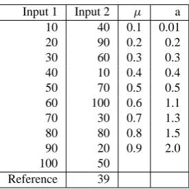
Table 1. Input 1 (NM) showing a systematic increase in in-tensity of sequential events and Input 2 (NM) showing a more disordered set of sequential events.
Input 1 Input 2 µ a
10 40 0.1 0.01
20 90 0.2 0.2
30 60 0.3 0.3
40 10 0.4 0.4
50 70 0.5 0.5
60 100 0.6 1.1
70 30 0.7 1.3
80 80 0.8 1.5
90 20 0.9 2.0
100 50
Reference 39
1997; McCray, 1969; Megill, 1971; Rose, 1987). To obvi-ate all of these difficulties and drawbacks, it is appropriobvi-ate to invoke Bayesian updating (see Appendix A).
Another result forNM,N1m1, andN2m2is that Eq. (3) reduces to
pnext(1)=
ra 1−µ2 ra 1−µ2
+µ2 (21)
pnext(2)=
µ2 ra 1−µ2
+µ2 (22)
3 Maximum Likelihood Estimation programs
To be able to address the questions asked in the Introduction one has to convert the mathematical formalism described in Sect. 2 into computer programs. In this section of the paper two programs for the maximum likelihood estimation proce-dure are introduced and the results for two different experi-ments (ordered sequences of observations) are discussed.
Of the two programs, one describes the situation including all parametersN, while the second program is appropriate for the special caseNM. Both programs are created via Open-Office using spreadsheets to achieve high user friend-liness.
3.1 The special case,NM
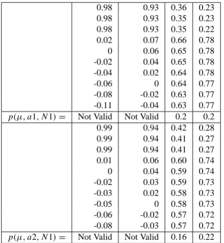
Table 2. This Table represents a small part of the calculation of the right side of Eq. (18). There are two sections each with 4 columns. In these sections one varies only one parameter (in this case the parameterµ; the columns in a section represent differentµ val-ues) while the other two parameters are constant (Note that one has different constant parameters in each section). The entries in the columns are the separate factors of Eq. (18). The last entries of the columns are the products of these factors.
0.98 0.93 0.36 0.23 0.98 0.93 0.35 0.23 0.98 0.93 0.35 0.22 0.02 0.07 0.66 0.78
0 0.06 0.65 0.78
-0.02 0.04 0.65 0.78 -0.04 0.02 0.64 0.78
-0.06 0 0.64 0.77
-0.08 -0.02 0.63 0.77 -0.11 -0.04 0.63 0.77
p(µ, a1, N1)= Not Valid Not Valid 0.2 0.2 0.99 0.94 0.42 0.28 0.99 0.94 0.41 0.27 0.99 0.94 0.41 0.27 0.01 0.06 0.60 0.74
0 0.04 0.59 0.74
-0.02 0.03 0.59 0.73 -0.03 0.02 0.58 0.73
-0.05 0 0.58 0.73
-0.06 -0.02 0.57 0.72 -0.08 -0.03 0.57 0.72
p(µ, a2, N1)= Not Valid Not Valid 0.16 0.22
anda, part of the user input as shown in Table 1 for two in-put sets. Both inin-put sets are for the same measured values but in a permutated order compared to a reference value set toIcut=39 (see Fig. 1). The difference that occurs when the order of the measured values is permuted is a change in the lowest number of observations for which the predictions make sense for a givenIcut. For Input 1 this value isM=5 and for Input 2 it isM=4, because one value has always to lie aboveIcut. An example for a variation of a parameter is given in Table 2, showing the variation ofµfor different, but fixed,a andN values for the 10 observed intensity val-ues. The program determines the bestµandavalues for the parameter interval chosen by the user (see Table 1 for the in-tervals and Fig. 2 for the best values for both inputs). These µandaparameters fit best to Eqs. (6).
The problem that occurs in this approach is that the user has to vary the parametersµandamanually. A great deal of time can be involved and for any of those chosen parameter intervals only the best values in this local area are obtained, which are not necessarily the globally best values. This defi-ciency can be repaired by an automatic search subroutine for calculating the best parameters, which is done in the second paper of this sequence (the mathematical procedure is pre-sented in Appendix B). With the obtained best values forµ
Fig. 1. Input 1(a) and Input 2(b) values in comparison with the reference intensity.
Fig. 2. Best values ofaandµ(Input 1(a) and (c) and Input 2(b) and (d);NM).
Fig. 3. Joint probability distributions (Input 1 (solid) and Input 2 (dot);NM) estimated for allM- see text for further description.
andathe program can determine the joint probability distri-bution functions for the events (measured values).
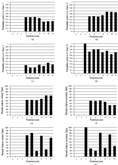
Fig. 4. Probability for the next event to lie in class 1 or class 2 (Input 1(a) and (b) and Input 2(c) and (d);NM). (a) and (b): Note that the first three events have intensities < Icut, while the fourth hasI4> Icut. Thus probability predictions can be given only for the fifth and higher events in the sequence. (c) and (d): Note that for the first event of Input 2I1> Icut, so the range of validity for the probability for the next event to lie in class 1 or class 2 starts with a prediction for the fourth measured value.
Fig. 5. Percent chance predicted point is in correct class (Input 1(a) and (b) and Input 2(c) and (d);NM).
Icut), given by Eq. (3), is illustrated for both inputs in Fig. 4, respectively. With a systematic increase in the number of measured values the probability that the event lies in class 1 decreases while the probability that the event lies in class 2 increases (Figs. 4(a) and (b). This effect is caused by the linear growth of the ordered intensity values in Input 1. For Input 2 (see Figs. 4(c) and (d)) one has a more chaotic be-havior of the data so that the decreasing/increasing effect of data Input 1 is now absent. With this program one is also able to calculate the probabilities that an event is either in
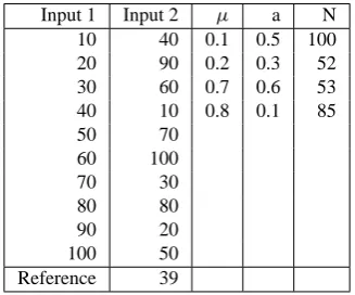
Table 3. Input 1 and Input 2 (N≥M).
Input 1 Input 2 µ a N
10 40 0.1 0.5 100
20 90 0.2 0.3 52
30 60 0.7 0.6 53
40 10 0.8 0.1 85
50 70
60 100
70 30
80 80
90 20
100 50
Reference 39
the correct or incorrect class as shown in Fig. 5 for Inputs 1 and 2, respectively. Figures 5(a) and (b) illustrate the fact that if more measured values are incorporated into the calcu-lations the higher is the probability to find an event to be in the correct class, which is again caused by the linear increase of the data values of Input 1. For data set 2 the probability to find an event in the correct class is between 15% and 80% (Figs. 5(c) and (d)). There is no specific pattern to be found. 3.2 The general case,N≥M
In the program for the general case finite values of the param-eterNare used, so Eq. (18) is the mathematical basis for the numerical variation calculations of the parametersN, µand a. The analytical procedure utilized in this program differs from the one used in the special case program given above. Instead of finding the maxima of Eq. (18) by calculating its partial derivations one finds these by direct variation of the parameters so thatpis as close to unity as possible for the prescribed values of the three input parameters. The three input boxes for the parametersµ, aandN are much smaller than for the special case program (see Table 3). The reason for this limitation of the input values is the rapid increase of the size of the program caused by every new parameter. Be-causeN≥Mthere are restrictions for the minimum value of N for the calculations to make sense. Those do not occur in the special caseNM.
Fig. 6. Best values ofa, µ and N (Input 1(a) and Input 2(b);
N≥M).
Fig. 7. Joint probability distribution (Input 1 (solid) and Input 2 (dot);N≥M) estimated for allM- see text for further description.
Icut) is illustrated in Figs. 8(a) and (b) and Figs. 8(c) and (d) for the data sets 1 and 2, respectively. The behavior is nearly the same as in the special case program (see Fig. 4) with the difference that the increase of the probability in Figs. 8(a) and (b) is not as extreme as in Figs. 4(a) and (b). The prob-ability that the events are in the correct or incorrect class is presented in Figs. 8(e) and (f) for Input 1 and Figs. 8(g) and (h) for Input 2. With a growing number of measured values the increase of the probability that the next data point is in the correct class is compared to the results from the special case program less powerful. In Fig. 8(g), no particular pattern can be found.
Fig. 8. Probability for the next event to lie in class 1 or class 2 (Input 1(a) and (b) and Input 2(c) and (d);N≥M). (a) and (b): Note that the first three events have intensities < Icut, while the fourth hasI4> Icut. Thus probability predictions can be given only for the fifth and higher events in the sequence. (c) and (d) Note that for the first event of Input 2I1> Icut, so the range of validity for the probability for the next event to lie in class 1 or class 2 starts with a prediction for the fourth measured value. In (e) - (h) the percent chance that the predicted point is in the correct class is presented (Input 1(e) and (f) and Input 2(g) and (h);N≥M).
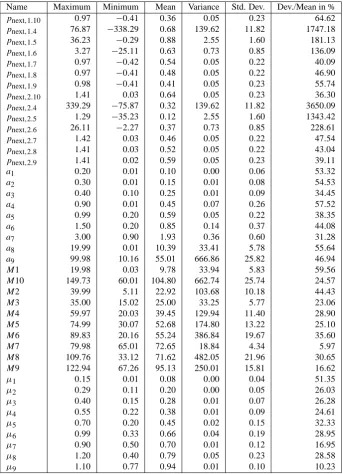
de-Table 4. Summary of the Monte Carlo simulation variables used together with ranges and statistical characteristics.
Name Maximum Minimum Mean Variance Std. Dev. Dev./Mean in %
pnext,1.10 0.97 −0.41 0.36 0.05 0.23 64.62
pnext,1.4 76.87 −338.29 0.68 139.62 11.82 1747.18
pnext,1.5 36.23 −0.29 0.88 2.55 1.60 181.13
pnext,1.6 3.27 −25.11 0.63 0.73 0.85 136.09
pnext,1.7 0.97 −0.42 0.54 0.05 0.22 40.09
pnext,1.8 0.97 −0.41 0.48 0.05 0.22 46.90
pnext,1.9 0.98 −0.41 0.41 0.05 0.23 55.74
pnext,2.10 1.41 0.03 0.64 0.05 0.23 36.30
pnext,2.4 339.29 −75.87 0.32 139.62 11.82 3650.09
pnext,2.5 1.29 −35.23 0.12 2.55 1.60 1343.42
pnext,2.6 26.11 −2.27 0.37 0.73 0.85 228.61
pnext,2.7 1.42 0.03 0.46 0.05 0.22 47.54
pnext,2.8 1.41 0.03 0.52 0.05 0.22 43.04
pnext,2.9 1.41 0.02 0.59 0.05 0.23 39.11
a1 0.20 0.01 0.10 0.00 0.06 53.32
a2 0.30 0.01 0.15 0.01 0.08 54.53
a3 0.40 0.10 0.25 0.01 0.09 34.45
a4 0.90 0.01 0.45 0.07 0.26 57.52
a5 0.99 0.20 0.59 0.05 0.22 38.35
a6 1.50 0.20 0.85 0.14 0.37 44.08
a7 3.00 0.90 1.93 0.36 0.60 31.28
a8 19.99 0.01 10.39 33.41 5.78 55.64
a9 99.98 10.16 55.01 666.86 25.82 46.94
M1 19.98 0.03 9.78 33.94 5.83 59.56
M10 149.73 60.01 104.80 662.74 25.74 24.57
M2 39.99 5.11 22.92 103.68 10.18 44.43
M3 35.00 15.02 25.00 33.25 5.77 23.06
M4 59.97 20.03 39.45 129.94 11.40 28.90
M5 74.99 30.07 52.68 174.80 13.22 25.10
M6 89.83 20.16 55.24 386.84 19.67 35.60
M7 79.98 65.01 72.65 18.84 4.34 5.97
M8 109.76 33.12 71.62 482.05 21.96 30.65
M9 122.94 67.26 95.13 250.01 15.81 16.62
µ1 0.15 0.01 0.08 0.00 0.04 51.35
µ2 0.29 0.11 0.20 0.00 0.05 26.03
µ3 0.40 0.15 0.28 0.01 0.07 26.28
µ4 0.55 0.22 0.38 0.01 0.09 24.61
µ5 0.70 0.20 0.45 0.02 0.15 32.33
µ6 0.99 0.33 0.66 0.04 0.19 28.95
µ7 0.90 0.50 0.70 0.01 0.12 16.95
µ8 1.20 0.40 0.79 0.05 0.23 28.58
µ9 1.10 0.77 0.94 0.01 0.10 10.23
fined by the user and not by an automatic mode of operation. So one can not be certain in gaining the most appropriate parameter values.
4 Discussion and Conclusion
This paper has developed an analytical description and nu-merical methods for future predictions of events in astro-physics that can be garnered from a sequence of observed events. To determine the possible future behavior of occur-ring events one first investigates general probability
consid-erations using a maximum likelihood estimation. The results received from the maximum likelihood estimation are further discussed for the approximation of the large number limit of possible events. The mathematical formalisms had to be transformed into computer codes, one, for a finite number system and one for a large number approximation as a spe-cial case of a finite number system.
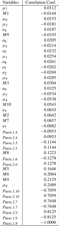
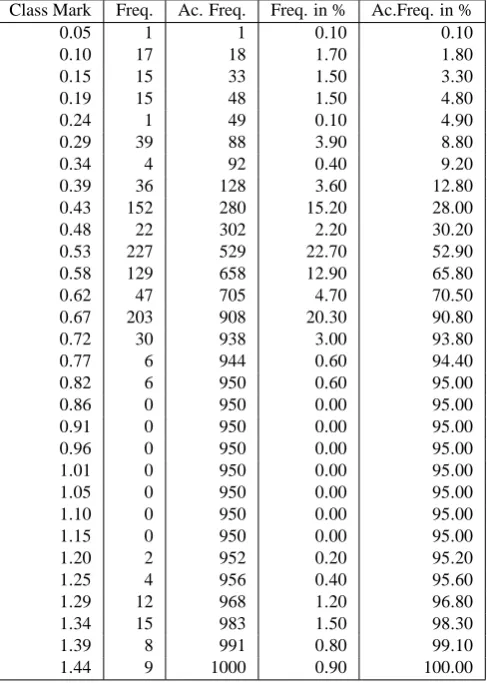
Table 5. Probability statistics for input pnext,2.8 showing the chances of findingpnext,2.8in given ranges as well as the cumu-lative probability of obtaining a value forpnext,2.8less than a spec-ified worth.
Variables Correlation Coef.
µ7 0.0112
M1 −0.0144
µ6 0.0153
µ3 −0.0181
a4 0.0187
M9 −0.0193
a6 0.0205
µ5 −0.0214
a5 0.0232
µ1 0.0254
a8 0.0261
a1 −0.0262
a2 −0.0269
µ9 0.0285
M3 0.0304
a9 0.0325
µ2 −0.0534
µ4 −0.0538
M10 0.0543
a3 0.0610
M2 0.0642
M7 0.0657
a7 −0.0682
pnext,1.4 −0.0953
pnext,2.4 0.0953
pnext,1.5 −0.1144
pnext,2.5 0.1144
M8 0.1223
pnext,1.6 −0.1278
pnext,2.6 0.1278
M5 0.1646
M6 0.2064
M4 0.2129
µ8 0.2489
pnext,1.10 −0.7059
pnext,2.10 0.7059
pnext,2.7 0.7648
pnext,1.7 −0.7648
pnext,2.9 0.8125
pnext,1.9 −0.8125
pnext,1.8 −1.0000
is why results are usually quoted to 1σ (occasionally 2σ). The cut intensity level,Icut, is, of course, precisely known because one can choose the value. If a particular member of the measured sequence has a mean intensityIi such that |Ii−Icut| ≤1σ then, with confidence, one can ascribe that member to either the class less than or greater than the cut. However, when the uncertainty onIi is sufficiently large that |Ii−Icut| ≥1σone does not know into which category the member is to be assigned. Accordingly, depending on the
Fig. 9. Sensitivity of the outputpnext,2.8in a Tornado Graph with the abscissa being the correlation coefficient range(−1,1). The largest values have the most influence on the sensitivity ofpnext,2.8 and are taken from Table 5.
value chosen forIcut, there will be corresponding uncertain-ties in the parametersN, µandaand also an uncertainty on assessing whether the (M+1)st intensity is predictable as being in the lower or upper classes. Fortunately, these prob-lems can be addressed readily using Monte Carlo procedures as follows. Given that one knows the uncertainty distribution around the mean on each of the measured values then one chooses the same distribution for a suite of Monte Carlo runs from which one can compute the likely membership classes, the average values and uncertainties forN, µand foragiven sequence of measurements, and the uncertainty on the prob-ability that the next value will lie above or below the Icut value. A numerical illustration of this Monte Carlo proce-dure is now given using data set 1.
That simulation was performed with 1000 Monte Carlo iterations for the input set (“Value”, µ, a) and the output set (pnext,1, pnext,2). Note that the output set starts with the fourth value ofpnext,1andpnext,2because the first three val-ues are less thanIcut. A continuously uniform distribution was used for the parameterµanda and a discrete uniform distribution for the parameter “Value”.
Fig. 10. Graph of the distribution forpnext,2.8due to uncertainties in parameters and input data.
most sensitive to changes in inputµ8(best value ofµusing eight measured values). The statistical data and the distribu-tion plot forpnext,2.8 are illustrated in Table 6 and Fig. 10. The most probable value forpnext,2.8is 0.52, but the range to half the peak value indicatespnext,2.8=0.52 +−0.120.18
, thereby providing some measure of the influence of uncertain data values and uncertain parameters on the predictability of the next event.
The programs as built include only 10 measurement value inputs. More data can be included in the programs but it was felt that 10 data points more than sufficed to illustrate the principles involved. In addition, in any future extension of the programs one should increase the number of classes for data points so that one can incorporate more information than that values lie either above or belowIcut.
In order to improve on the procedure itself for assessing the probability of predicting future events one must move from a user-intensive, and limited, manual input of param-eter estimates to procedures that provide systematic updat-ing based on priors. In the next paper we discuss the Bayesian update method and the systematic parameter deter-mination procedure as relevant improvements of predictabil-ity for which basic mathematical developments are given in Appendix A and Appendix B.
The relevance of the prediction procedure for individual sources of high energy photons is that it enables one to sort out whether a source is truly weak or whether one is merely observing on the edge of a focused beam for a strong source. In addition, because the generation of pulses of high energy photons from individual objects appears to be somewhat ran-dom in time, the present procedure allows one to at least es-timate from a given number of observed pulses a minimum number one is likely to observe.
One should be careful not to apply the procedure to all high energy photon sources simultaneously because then one has no idea of the mixture of long-lived and short-lived
ob-Table 6. Correlation coefficients (sensitivity data) for the proba-bility that the next event is in class 2 withM=8,pnext,2.8, orga-nized from lowest to highest in absolute value. The variablesµi andai are the bestµandaparameters fori measured valuesMi (i=1, ...,10).
Class Mark Freq. Ac. Freq. Freq. in % Ac.Freq. in %
0.05 1 1 0.10 0.10
0.10 17 18 1.70 1.80
0.15 15 33 1.50 3.30
0.19 15 48 1.50 4.80
0.24 1 49 0.10 4.90
0.29 39 88 3.90 8.80
0.34 4 92 0.40 9.20
0.39 36 128 3.60 12.80
0.43 152 280 15.20 28.00
0.48 22 302 2.20 30.20
0.53 227 529 22.70 52.90
0.58 129 658 12.90 65.80
0.62 47 705 4.70 70.50
0.67 203 908 20.30 90.80
0.72 30 938 3.00 93.80
0.77 6 944 0.60 94.40
0.82 6 950 0.60 95.00
0.86 0 950 0.00 95.00
0.91 0 950 0.00 95.00
0.96 0 950 0.00 95.00
1.01 0 950 0.00 95.00
1.05 0 950 0.00 95.00
1.10 0 950 0.00 95.00
1.15 0 950 0.00 95.00
1.20 2 952 0.20 95.20
1.25 4 956 0.40 95.60
1.29 12 968 1.20 96.80
1.34 15 983 1.50 98.30
1.39 8 991 0.80 99.10
1.44 9 1000 0.90 100.00
jects for which one is attempting to apply statistics. The as-sumptions of independence of pulses and non-recurring peri-odic nature from an individual source are the basic linchpins of the procedure and should not be violated. But within that framework, one has now available a set of procedures that en-able one to provide assessments of future chances of observ-ing events from a source and of determinobserv-ing what percentage are likely to be weak or strong intrinsically.
Appendix A Bayesian updating
a from which individual values are chosen for the Monte Carlo runs, subject only toN≥M,0≤µ≤1 anda >0. Let the joint probability distribution for these underlying choices be Pk(α). Now suppose one is interested in adding the next observed event,(k+1). Bayes theorem (Jaynes, 1978; Lerche, 1997; Harbaugh et al., 1977; Feller, 1968) then states that for the given set{α}of Monte Carlo run parameters chosen the conditional probabilityPk+1(α)that one knows event(k+1)is provided through
Pk+1(α)=
Pk(α)p(k+1;α)
P
αPk(α)p(k+1;α)
(A1) Thus one has updated the probability distribution of theα so that one is progressively changing the probability that a givenαtriad(Nα, µα, aα)will more closely honor the ob-served events. Note from Eq. (18), that
p(k+1;α)=p(k;α)×
[kk+1,1ra(Nsin2θ−γk+1)+kk+1,2ra(Ncos2θ−δk+1)] ra(Nsin2θ−γ
k+1)+Ncos2θ−δk+1)
≡p(k;α)ω(k+1;α) (A2)
with
γk+1=γk+kk+1;1, δk+1=δk+kk+1;2 (A3) so that one merely has to calculate the Monte Carlo suite of values for the bracketed factor in Eq. (A2) once for each event. Bayes updating then proceeds iteratively by adding the next event,k+2, and so, in general, one obtains after all Mevents have been added
PM(α)=
PM−1(α)p(M−1;α)
P
αPM−1(α)p(M−1;α)
(A4) and so providing, for each triadα chosen, the probability PM(α)that the set ofαcomes as close as possible to hon-oring all the observed events. What the Bayes updating does not do is provide information on whether the set{α} cho-sen reprecho-sents the best possible fit. The point is that a finite suite of Monte Carlo calculations is involved. Thus one has chosen a finite number of values for(Nα, µα, aα).
The Bayes updating procedure indicates which of these fi-nite number of values has the highest relative probability of honoring all the data but provides no information on non-chosen values of the parameters. Thus the absolute highest probability of honoring all the events may depend on other values than those chosen. One could iterate many times the whole Monte Carlo scheme, and associated Bayesian updat-ing, with different random choices of the parameter triad (N, µ, a)from the underlying distributions of the parame-ters. In this way one would construct (eventually!) a dense set of parameter values and so identify almost surely the best parameter triad honoring most closely the observed events. However, such a procedure is not only computer intensive but may also be futile. The point is that in constructing the basis
probability distribution functions for the Monte Carlo suite operations one has not only to ensure that one honors the physical requirements onN (≥M), µ(0≤µ≤1)anda(>0) but one also has to choose maximum values for N anda, sayNmaxandamax. It can happen that the values ofN and a needed to satisfy the observed events lie greater than the chosen valuesNmaxand /oramax.
What one needs is a procedure to supplement the Bayes updating that systematically and deterministically will obtain the parameter triad (N, µ, a) that will allow pM(M;N, µ, a) to honor the ordered sequence of M ob-served events, starting with the triad determined from the Bayes updating procedure that has the highest relative prob-ability, but allowing determination of parameter values not chosen in the original Monte Carlo suite of operations. In addition, any such systematic procedure must deter-mineNmax andamaxso that the highest absolute probabil-ity for p(M;N, µ, a) is contained in Nmax≥N≥M and amax≥a≥0. This aspect of the problem is addressed in Ap-pendix B.
Appendix B Systematic determination of parameter values
Let the triad value0be that with highest relative probabil-ityp(M;0)of satisfying allM observed events obtained from Bayesian updating. Now if the situation were to match perfectly with the observedM events then not only would P (M;0)be unity but so, too, would each individual factor probabilityp(k;0) (k=1, ..., M) (see Eq. (A2)). To the extent that there is not perfection,p(k;0)will differ from unity. To determine the parameter triad that will match the Mobservations most closely define
χ2()=M−1 M
X
k=1
[1−p(k;)]2 (B1)
because, with perfection,p(k;best)=1. Then one wishes to obtain a systematic procedure so thatχ2()is minimized, starting with the Bayesian updated triad 0, and allowing Nmax andamax to range outside of the values assigned in the Bayesian update method. Such a systematic procedure can be developed as follows. BecauseN≥M, it is useful to writeN=M10xwherex≥0, and considerxas a basic vari-able. Then suppose, initially, one takes each component of the vector parameterq=(χ , µ, a)to lie in an initial chosen rangeqmax(i) ≥q≥qmin(i) wherei=1,2 or 3 according as one handles withχ , µora, respectively. Then set
sin2θ(i)= q (i) max−q(i) qmax(i) −qmin(i)
(B2)
with the initial value sin2θ0(i)=(qmax(i) −q0(i))/(q (i)
iteration scheme (Lerche, 1997) designed to ensure conver-gence to the smallest value ofχ2in Eq. (B1) is
θn(i)+1=θn(i)exp −δn(i) ∂χ 2/∂θ(i)
n
∂χ2/∂θ0(i) !
(B3)
whereδn(i)=1 forn=0 and
δn(i)=
θ
(i) n −θn(i)−1
τ−1Pτ
j=1
θ
(i) n −θn(i)−1
for n6=0;
and where the derivatives are given by the approximate eval-uation
∂χ2
∂θn(i)
= [χ2(θn(1), ..., θn(i)(1+β), ...)
−χ2(θn(1), ..., θn(i), ...)]/βθn(i) (B4) with |β| 1. Note that the iteration scheme represented through Eq. (B3) has the following properties:
1. It guarantees thatχ2will be either smaller or the same after each iteration;
2. It guarantees that all parameters will remain within the boundsqmax(i) ≥q(i)≥qmin(i) for all iterations;
3. Because of the factor δn(i), the iteration scheme treats first with those parameters that are causing the greatest change inχ2, while minimizing the influence of other parameters until all parameters are causing essentially the same change inχ2;
4. If sin2θn(i)→1 (0) then the iteration scheme is in-forming one that either the chosen lower (upper) value qmin(i)(qmax(i) ) is too large (sin2θn(i)→1) or too small(sin2θn(i)→0)and must be decreased (increased), thereby providing the necessary information on which direction to change any initial chosen parameter ranges; 5. The scale value∂χ2/∂θ
(i) 0
is best changed after a finite
number,Q, of iterations by replacingθ0(i)byθQ(i). Prag-matically it is superior in terms of convergence speed to performQiterations twice with the update of the scale value after the firstQiterations rather than perform 2Q iterations once with the original fixed scale value. Coupled with the Bayesian update procedure, this systematic method then guarantees one obtains the values ofN, µand a most consistent (smallest χ2) with the observed ordered event sequence. Once the values forN, µanda are so de-termined then one can use Eq. (3) to evaluate the probability that the next event is in classj. As the intensity level,Icut, is progressively raised the probability that the next event will lie aboveIcutis systematically lowered. But, at each level ofIcut, one obtains estimates of the total number,N, of pos-sible observable events together with the power index,a, as
well asN1/(N1+N2)≡ µ2. The total number,N, of pos-sible observable events, as well as the observability indexa, should likely be independent of the chosen intensity levelIcut if the observed number of events,M, is representative of the totalN. Numerical implementation of Appendices A and B is considered in the second paper of this series.
Acknowledgements. This work was supported by the DFG under SFB 591 and also by the award of a Mercator Professorship to Ian Lerche. We are most grateful for this support and also for the courtesies shown us by Prof. Reinhard Schlickeiser during our stay in Bochum.
Edited by: H. Fichtner
Reviewed by: two anonymous referees
References
Aldrich, J.: R. A. Fisher and the making of maximum likelihood 1912-1922, Stat. Science, 12, 162–167, 1997.
Arps, J. J., Smith, M. B., and Mortada, J.: Relationship between proved rese and exploratory effort, J. Pet. Technol., 23, 671–675 1971.
Cronquist, C.: Reserves and probabilities?synergism or anachro-nism?, J. Pet. Technol., 43, 1258–1264, 1991.
Dingus, B. L. and Catelli, J. R.: EGRET Detections of the High-est Energy Emission from Gamma-Ray Bursts in: Abstracts of the 19th Texas Symposium on Relativistic Astrophysics and Cos-mology, 63, 1998.
Feller, J.: Elements of probability theory, McGraw-Hill, Englewood Cliffs, 1–2, 1968.
Fisher, R. A.: Theory of statistical estimation, Proc. Cambridge Phi-los. Soc., 22, 700–725, 1925.
Fisher, R. A.: Two new properties of mathematical likelihood, Proc. Roy. Soc., 144, 285–307, 1934.
Fishman, G. J. and Meegan, C. A.: Gamma-Ray Bursts, Annu. Rev. Astron. Astrophys., 33, 415–458, 1995.
Frail, D. A., Kulkarni, S. R., Sari, R., Djorgovski, S. G., Bloom, J. S., Galama, T. J., Reichart, D. E., Berger, E., Harri-son, F. A., Price, P. A., Yost, S. A., and Diercks, A.: Beaming in Gamma-Ray Bursts: Evidence for a Standard Energy Reservoir, Astrophys. J. Lett., 562, L55, 2001.
Harbaugh, J. W., Doveton, J. H., and Davis, J. C.: Probability meth-ods in oil exploration, Wiley, New York, 1977.
Hurley, K., Sari,R., and Djorgovski, S. G.: Cosmic Gamma-Ray Bursts, Their Afterglows, and Their Host Galaxies, astro-ph/0211620, 2002.
Jaynes, E. T.: Where do we stand on maximum entropy? in: The Maximum Entropy Formalism, MIT Press, Cambridge, MA, 15– 118, 1978.
Lerche, I.: Geological risk and uncertainty in oil exploration, Aca-demic Press, San Diego, 1997.
Lumley, J. L.: Stochastic tools in turbulence, Academic Press, New York, 1970.
McCray, A. W.: Evaluation of Exploratory Drilling Ventures By Statistical Decision Methods, J. Pet. Technol., 21, 1199–1209, 1969.
Panaitescu, A. and Kumar, P.: Fundamental Physical Parameters of Collimated Gamma-Ray Burst Afterglows, Astrophys. J. Lett., 560, L49, 2001.
Piran, T., Kumar, P., Panaitescu, A., and Piro, L.: The Energy of Long-Duration Gamma-Ray Bursts, Astrophys. J. Lett., 560, 167–169, 2001.
Piran, T.: Gamma-Ray Bursts and the Fireball Model, Phys. Rep., 314, 575–667, 1999.
Piran, T.: Gamma-ray Bursts - A Puzzle Being Resolved, Phys. Rep., 333, 529–553, 2000.
Piran, T.: The physics of gamma-ray bursts, Rev. of modern physics, 76, 1143–1211, 2004.
van Paradijs, J., Kouveliotou, C., and Wijers, R. A. M. J.: Gamma-Ray Burst Afterglows, Annu. Rev. Astron. Astrophys., 38, 379– 425, 2000.