Hydrothermal Processes

V

o

lu

m

e 4

, n

u

m

be

r 1

|

A

pr

il 2

01

H

U

BE

RT L

. B

A

R

N

ES

HUBERT L. BARNES

is an Emeritus, Distinguished Professor of Geochemistry in the Geosciences Department of the Pennsylvania State University. His research over the last 7 decades has concentrated on hydrothermal processes of geothermal and ore-forming systems. His methods of investigation depended upon both experimental techniques at high pressures and temperatures and thermodynamic and kinetic evaluations. The results were described in about 200 publications and six books that include editing over three decades three volumes that became the principal sources in the «Geochemistry of Hydrothermal Ore Deposits» fittingly termed the G(h)OD books. His scientific career began at M.I.T. as a student and than as a Fellow of the Geophysical Laboratory of the Carnegie Institution in Washington, D.C. Later, he moved to Penn State University as a Professor of Geochemistry and there he also served as Chairman of the Geochemistry and Mineralogy Program and as Director of the Ore Deposits Research Section. His long career included being the President of the Applied Research and Exploration Corporation in Pennsylvania and being a consultant for more than 30 corporations in work that produced four patents. Within the geochemical community, Hu became the President of the Geochemical Society and he was the one who initiated its Goldschmidt Conferences, now the principal annual meeting of geochemistry in the world. The publication of this Geochemical Perspectives issue coincides with the 25th _{anniversary celebration of the Goldschmidt Conference series in 2015} in Prague. A detailed biography of Hu with his many achievements can be found at the end of the issue.

Ta ke n n ea r t he s ou th ea st c oa st o f K am ch at ka i n m id - s um m er , 1 99 5.

HU

BE

RT L

. B

AR

N

ES

Hydrothermal

Processes

L

iane

G. B

enninG University of Leeds, UK & GFZ, Germany

Editorial Board

T

im

e

LLioTT University of Bristol, UK

e

ric

H. o

eLkers

CNRS Toulouse, France & University College London, UK

s

usan

L.s. s

Tipp

University of Copenhagen, Denmark

Editorial Manager

m

arie

-a

ude

H

uLsHoff

Graphical Advisor

J

uan

d

ieGo

r

odriGuez

B

Lanco University of Copenhagen, Denmark Each issue of Geochemical Perspectives

pre-sents a single article with an in-depth view on the past, present and future of a field of geochemistry, seen through the eyes of highly respected members of our community. The articles combine research and history of the field’s development and the scientist’s opinions about future directions. We welcome personal glimpses into the author’s scientific life, how ideas were generated and pitfalls along the way.

Perspectives articles are intended to appeal to the entire geochemical community, not only to experts. They are not reviews or monographs; they go beyond the current state of the art, providing opinions about future directions and impact in the field.

Copyright 2015 European Association of Geochemistry, EAG. All rights reserved. This journal and the individual contributions contained in it are protected under copy-right by the EAG. The following terms and conditions apply to their use: no part of this publication may be reproduced, translated to another language, stored in a retrieval system or transmitted in any form or by any means, electronic, graphic, mechanical, photo-copying, recording or otherwise, without prior written permission of the publisher. For information on how to seek permission for reproduction, visit:

www.geochemicalperspectives.org

or contact [email protected]. The publisher assumes no responsibility for any statement of fact or opinion expressed in the published material.

ISSN 2223-7755 (print) ISSN 2224-2759 (online) DOI 10.7185/geochempersp.4.1 Principal Editor for this issue

Liane G. Benning, University of Leeds, UK & GFZ, Germany

Reviewers

Martin Schoonen, Stony Brook University, USA Terry Seward, Victoria University of Wellington, New Zealand

Cover Layout Pouliot Guay Graphistes

Typesetter Info 1000 Mots

Printer Deschamps impression

ABOUT THE COVER Terraces of hydrothermally deposited travertine (CaCO3) in Mammoth Hot Springs of Yellowstone National Park, northwestern Wyoming. Typical temperatures of the solutions in the springs are below boiling, typically about 80 ºC.

www.eag.eu.com

Geochemical Perspectives is an official journal

of the European Association of Geochemistry

The European Association of Geochemistry, EAG, was established in 1985 to promote geochemistry, and in particular, to provide a platform within Europe for the presentation of geochemistry, exchange of ideas, publications and recognition of scientific excellence.

Officers of the EAG Council

President

Liane G. Benning,

University of Leeds, UK & GFZ, Germany Vice-President

Bernard Marty,

CRPG Nancy, France

Past-President

Chris Ballentine,

University of Oxford, UK

Treasurer

Karim Benzerara,

University Pierre et Marie Curie, France Secretary

Andreas Kappler,

University of Tübingen, Germany

Goldschmidt Officer

Eric Oelkers,

CNRS Toulouse, France & University College London, UK Goldschmidt Officer

Antje Boetius,

University of Bremen, AWI Helmholtz & MPG, Germany

J

anne

B

LicHerT

-T

ofT

CONTENTS

Foreword . . . III

Acknowledgements . . . V

Hydrothermal Processes: The Development of Geochemical Concepts

in the Latter Half of the Twentieth Century . . . 1

Abstract . . . 1

1 . Introduction . . . 3

1 .1 My Personal Journey . . . 3

1 .2 Fascination with Ore Deposit Enigmas . . . 11

2 . The Mystery of Ore-Forming Environments: Which Parameters to Resolve? . . . 12

2 .1 Redox Conditions . . . 12

2 .2 Acidity . . . 13

3 . Experimental Investigation of Transport Chemistry . . . 17

3 .1 The Urgency to Understand Metal Complexes in Solution: Hard and Soft Choices . . . 20

3 .2 Vapour Transport – Another Horizon for the Future . . . 26

4 . Deducing the Conditions where Ores Form . . . 28

4 .1 How the Geochemistry of Quartz Developed into the Most Valuable Geothermometer . . . 28

4 .2 The Nature of Sphalerite Geothermometry and Geobarometry . . . 31

4 .3 Evidence of Environmental Conditions from Ubiquitous Iron Sulphides . . . 33

5 . Geothermal Systems . . . 45

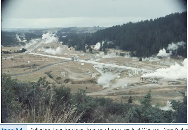
5 .1 Wairakei, New Zealand . . . 48

6 . Low Temperature Hydrothermal Deposits . . . 55

6 .1 The Upper Mississippi Valley District (UMVT) . . . 55

7 . Epilogue . . . 73

The Nature of Our Profession . . . 77

References . . . 78

Glossary . . . 88

Index . . . 90

FOREWORD

I initially got to know about Hu Barnes’ work in the mid nineties while a PhD student at ETH Zürich and as I read the 2nd _{edition of “Geochemistry of}

Hydro-thermal Ore Deposits” . The various chapters in that book taught me that Hu and his collaborators have in many ways throughout the latter part of the 20th

century revolutionised experimental hydrothermal ore deposit geochemistry and helped us better understand how our planet’s ore deposits formed . I wanted to learn from that .

wanted to (at least in part) become like him . During my tenure at Penn State as one of his last 2 postdocs (Rick Wilkin, now at EPA being the other one) I was in awe because above the door of our office were the name tags of so many of the great scientists in geochemistry and they all had worked with Hu at Penn State . It was big shoes to step into but naturally I did not only learn hydrothermal experimental tricks from Hu but also many research life tricks that have served me well over the years . Hu and I have kept in touch since I left Penn State; these memories as well as Hu’s many achievements and contributions convinced me that I had to persuade him to write an issue for Geochemical Perspectives . I wanted him to describe his geochemical story for the future generations . I also wanted the publication of this Geochemical Perspectives to coincide with the 25th _anniversary

of the annual Goldschmidt Conferences in Prague because Hu was more than just instrumental in initiating this conference series (see Section 7) .

I very much enjoyed editing this with Hu and I hope you enjoy reading it .

ACKNOWLEDGEMENTS

I very much appreciated many editorial suggestions that resulted in valuable revisions to the manuscript of this issue of Geochemical Perspectives . Extensive editing was contributed by Liane G. Benning, University of Leeds and now at the Geoforshungs Zentrum in Postsdam, and Dave Wesolowski, U .S . Oak Ridge National Laboratory . Sections were reviewed by Martin Schoonen, U .S . Brookhaven National Laboratory; Terry Seward, Victoria University, Wellington, New Zealand; Antonio Lasaga; Roger McLimans, DuPont Corporation; Jim Murowchick, University of Missouri-Kansas City and Mary Barnes, Penn State University .

Hubert L. Barnes

HYDROTHERMAL PROCESSES:

THE DEVELOPMENT OF

GEOCHEMICAL CONCEPTS

IN THE LATTER HALF OF THE

TWENTIETH CENTURY

_ABSTRACT

This GeochemicalPerspectives follows along my path through the evolution and development of hydrothermal concepts as they became established during the latter half of the twentieth century, from conjecture through established precept . A powerful stimulus for the developments was a keen scientific interest in the genesis of hydrothermal ore deposits shared commonly by my colleagues, both geochemists and economic geologists . Underlying that interest was our optimistic belief that a fundamental understanding of ore-forming processes should have practical applications for mineral exploration .

Furthermore, we found that information on the high P-T volumetric and thermo-dynamic behaviour of volatiles like CO2, CH4, H2S, SO2, and especially H2O were

incomplete for applications which ideally extend to about 1,000 ºC and 10,000 bars . This resulted in extensive experimental investigations internationally by geochemical laboratories that painstakingly provided much of the fundamental new data still currently used .

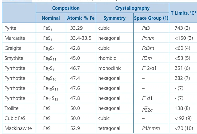
That crucial, advanced chemical information could be applied effectively only if the physical conditions (P, T) of the environments where ores had formed were more accurately identified . To better resolve these temperatures and pres-sures, a series of geothermometers and geobarometers were invented and tested on various settings . Two of these, the quartz geothermometer and the sphalerite (ZnS) geobarometer, are special in that they are flexibly adaptable to a variety of mineral deposits . Their attributes favour relatively easy application so I have selected them for a more thorough examination . Another family of highly useful geothermometers are dependent upon the unique characteristics of the ubiqui-tous iron sulphides . There are more than seven of these sulphides and most ore deposits contain more than one of them . These sulphides are especially important as precise indicators of the environmental conditions where they crystallised, not only due to their occurrence within a deposit but also by differences in their solid solution composition and in morphology . We found that variations among the characteristics of the iron sulphides were largest precisely within the range of conditions of chemistry, temperature, and pressure where ores crystallise, attributes which made these indicators extremely valuable .

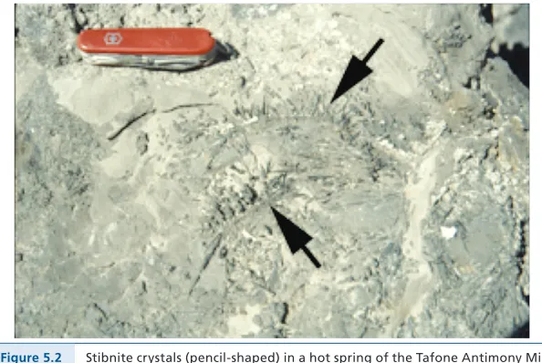
The nature of hydrothermal processes found from the rock record through mineralogical evidence on ore deposits was naturally supplemented by data from investigations of modern and active geothermal systems . Our initial consid-eration was to ascertain whether geothermal processes and hydrothermal ore genesis were related phenomena . In fact, it turned out that their ranges of temper-atures and pressures and their deduced lifetimes were identical . Therefore, the measured solution flow rates and compositions of modern geothermal systems provided excellent baselines for modelling what must have transpired in ore-forming environments, which are simply ancient geothermal sites .

continued to provide increased resolution . These techniques and new data sets led to more accurate and precise thermodynamic descriptions of the complexes, which have been used to calculate, and then plot, variations in solubility as a function of oxidation state (log a_O2) and of pH at pertinent temperatures and pressures . Potential causes of ore deposition are implicit in such diagrams .

The maturity of our understanding of hydrothermal processes could be tested most readily against criteria from the lowest temperature and pressure ore deposits, the Mississippi Valley type zinc-lead ores . The extensive database for those in Illinois, Iowa and Wisconsin made that district ideal as a model . There, the ore-depositing solutions arrived about 270 million years ago from their source in the contemporaneously uplifted southern Appalachian Moun-tains . They flowed northward through the Illinois Basin becoming heated, highly saline, with a reduced oxidation state, slightly alkaline to neutral acidity, and with solute concentrations apparently especially rich in iron, barium, zinc, and lead . It was effectively a hot groundwater that flowed at about 11 metres per year from its source for 1100 km to the district to precipitate sulphides within an horizontal 35 metre depth range about 1 km deep . The mineral paragenetic sequence revealed that slight oxidation was sufficient to cause sulphide deposi-tion dominantly at 125 ± 25 ºC and for sphalerite (ZnS) at a yearly rate of coating of about 0 .2 μm . Four independent methods agreed that the process continued for about 0 .25 million years . However, the aqueous complexes have not yet been identified for certain . Those metal-carrying aqueous species must have provided sufficient solubility to form deposits over an area of 10,000 square kilometres . Because the very regular banding in sphalerite could be correlated over a very large area implies that there must have been continuing, recycling climate control of that ore-forming hydrothermal system . This observation is intriguing and still unresolved and calls for additional studies and a mechanistic explanation .

1.

_INTRODUCTION

My Personal Journey

In this Perspective of the evolution of hydrothermal concepts during the last half of the twentieth century, my (Fig . 1 .1) purpose is to provide an overview of how the field developed and the consequences to my life especially through extensive collabo-ration with colleagues over the five decades . Far more detailed technical discussions of many of the concepts can be found in the three progres-sive editions of Geochemistry of Hydrothermal Ore

Deposits published in 1967, 1979, and 1997, that

cover a span of three decades of our slowly devel-oping comprehension of ore formation .

While preparing this Geochemical Perspec-tives, a compelling conclusion became evident, that the nature and capabilities of colleagues are crucial to the evolution of a career . They provide stimulation and advice on discovering and evaluating opportunities at each juncture in life .

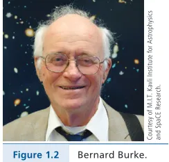
At Lexington, Massachusetts High School in the 1940’s, welcome distrac-tions were sports, for me especially in track and football . My friend Bernard Burke (Fig . 1 .2) was a compatriot who was active in the same sports and also in playing the violin . He had additional virtues that gradually became more appre-ciated . His father, a math teacher at Rindge Technical High School, continued to challenge Bernard intellectually . The stimulus was contagious as we became competitors academically and companions in the social activities at school and in weekend violin and composing lessons at the South End Music School . Those happy lessons led to considering music as a profession but a new violinist at the Music School became proficient with Beethoven’s violin concerto in only two years, way beyond my multi-year competence . Bernard and I both concluded that science was equally enter-taining and that in nearby Cambridge, the Massachusetts Institute of Technology (M .I .T .) might be the route to interesting lives maybe as wealthy consultants . That dream led through undergraduate years at M .I .T . However, instead of following our financial inclinations, we both

1.1

Figure 1.1 Hu Barnes.

Co ur te sy o f M .I. T. K av li I ns tit ut e f or A st ro ph ys ic s an d S pa CE R es ea rc h.

became research-oriented, Bernard eventually as William A .M . Burden Professor of Astrophysics at M .I .T . and I as Distinguished Professor of Geochemistry at Penn State . My route there was the product of successive optimised choices .

The students entering M .I .T . with us in 1946 were predominantly veterans returning from World War II . They carried experiences that often gave academic advantages unusual for entering students, even to that Institution . Their level of performance meant that green high school students faced an intellectual transi-tion that overwhelmed some quite intelligent colleagues who sadly gave up and transferred . The more stubborn types gradually adjusted to the time and perfor-mance demands, eventually to our benefit . Like Bernard, my major initially was physics . That field seemed to be fairly prosaic compared to an elective course in geomorphology taught by Prof. F.K. Morris . His skill with coloured chalk gave us picturesque landscapes on the room’s three blackboards by the end of each period . The class, mostly of taciturn veterans, often applauded spontaneously at the conclusion of his lectures . His stories of geologic mapping in the wilds of Outer Mongolia added to the conviction that I should change majors to geology . My addiction to rock climbing and camping reinforced that choice and added to the inducement of probable exotic travel .

In the meantime, a job provided some income, ten hours per week as a technician in the Biology Department of M .I .T . There the principal effort was constructing, in a superb machine shop, the stainless steel body of one of the initial artificial kidneys under the direction of Prof. D.F. Waugh . Those were long days . Besides that employment were normal lectures, interminable homework plus commuting with buses and subway to M .I .T . which consumed the available hours but taught a capability of lifelong value – going to sleep whenever no action was required . For example, while standing in a subway car and holding onto its passenger hand straps, dozing was automatic . Sleep often arrived but ended sometimes with consternation by falling onto the lap of someone lucky enough to have captured a rare empty seat .

An example of an Outing Club-stimulated activity was a particular mid-winter tour

during the 1948 term break by three sophomore geology majors: Fred Barker from

Seekonk, Massachusetts, Robert (Bob) Leonard from Manville, New York, and me from

Lexington, Masschussetts . On Thursday, January 29, Bob and I left M .I .T . by

hitch-hiking with the intent of meeting Fred at Pinkham Notch, New Hampshire to climb

Mount Washington together . Being impecunious students, we minimised our costs by

free hitchhiking . Bob and I carried army surplus packs containing for each of us two

sleeping bags to be nested, spare clothes, flashlights, matches, a canteen, cooking kits, some food and a guidebook . The packs each weighed 80 lbs (36 kg) . I wore long johns,

wool hunting pants, a Bean’s Chamois shirt, a wool mackinaw, and rubber boots . Bob

had field boots, heavy pants, and a windproof jacket . We both carried crampons and Maine-style, tear-drop-shaped snow shoes about 4 .5 feet (1 .4 m) long, obtained from an army surplus store at minimal price .

Together with the packs and snowshoes, we made a sizable load so hitchhiking was very slow as most vehicles simply could not take us on board . The consequence

was that Bob and I covered during the first day only 2/3 of the distance to our goal,

Pinkham Notch, and at about dark, gave up and asked at a New Hampshire farm-house if we could sleep in their garage overnight . Having had no dinner and lying on their concrete floor was not a comfortable night .

Friday morning was snow-free but bitterly cold . Having no alternative, we started hitchhiking soon after daylight . Eventually, a friendly pickup driver offered us a ride if we would load ourselves into the back of his truck . Although that offered no chance for breakfast and it was downright windy and frigid in the back of the truck, we climbed aboard . In a few hours and with successive truck rides, we arrived near mid-day at Pinkham Notch where there was a fresh, deep snow pack .

Our immediate objective was to climb the Fire Trail (now the Tuckerman Trail) up to Hermit Lake Shelter in Tuckerman Ravine where we planned to camp as a base for later climbing, first up Lion Head bluff, then across Alpine Garden, and finally up the top cone of the mountain (Fig . 1 .3) . However, lack of nourishment, the deep soft snow, the heavy packs, and the awkward snow shoes slowed the hike to a crawl . About half way up the trail, we ran out of energy and had to eat something . The only edible item in our packs not requiring cooking was a package of Dromedary dried dates . Because the package was frozen and our hands were stiff with the cold, we soon found that the only solution was to break the container in half and eat it, dates, cardboard, cellophane and all .

Fred joined us at the Hermit Lake three-sided shelter (Fig . 1 .4), having used his skis to

negotiate the Fire Trail . The shelter was oriented with an open fourth side toward the mountain to limit the fetch for gusty winds . In the open side was a rough, loose-stone fireplace where smoke from the fire was vented away from the interior . However, the heat produced by rapid burning of dead branches was not enough to have much effect on the shelter’s temperature . The fire was crucial to prepare a very much needed hot dinner as quickly as our cold, stiff hands would allow .

Figure 1.3 Trails leading to Mt. Washington, New Hampshire. From the Pinkham Notch Visitors Center to the Hermit Lake Shelter is 2.4 miles (3.9 km).

were warmed in our pockets or at the fireplace . It was not a quiet place . Besides the roar of the wind through the trees, there often were cracks like gun shots that we blamed on frost in the trees . We wondered if the temperature was not exceptionally low to produce such natural tympani .

Toward the interior back of the shelter, the dirt floor was mostly free of snow . To avoid the frozen ground, a thick stack of evergreen branches served as rough, fragrant bunks . Nevertheless, even using two sleeping bags, we were so chilled that by the middle of the night, we had to climb out of our sleeping bags and exercise to generate some body heat . Of course, the wind had long since blown out any embers in the fireplace . Frostbite in our feet was a concern even during daylight because my rubber boots were surely poor insulation .

At daylight, we were anxious to build a fire for heat and breakfast . While collecting more firewood, we found farther up the ravine a small, locked, emergency shed named “Howard Johnson” on our maps . It had a recording thermometer which revealed our night had just dropped to -29° F (-34 ºC) with a wind chill much colder .

After breakfast, Bob and I donned our snowshoes and Fred clipped on his skis to climb

Figure 1.4 From left, me, Bob (with ski poles), and Fred leaving Hermit Lake Shelter to climb nor thward along Lion Head Trail here at the upper left rear (January 31,

1948).

Figure 1.5a Bob on the wind-packed slope of Alpine Garden See his shadow in a bright, sunny day (Januar y 31, 1948).

Figure 1.5b Looking south down toward Tuckerman Ravine from the turnaround point on the summit cone. Note the long shadows of the sunny, but late after-noon on January 31, 1948.

registered at the lodge, especially when the summit temperature had just fallen within two degrees of the record low of -50 °F (-46 ºC) . Also, he mentioned that the global record wind velocity for a half century, 231 mph (372 kph), had been measured on that summit . Due to respect for frequently stormy winds, the Summit Observatory is anchored by chains . Then he related accounts of several not-so-pleasant disasters under situations similar to our adventure with an added observation that we had been lucky, especially with snow-free weather .

Figure 1.5c Tuckerman Ravine on Mount Washington, New Hampshire. A more recent, mid-spring photo of Tuckerman Ravine showing the near vertical headwall used only by very expert skiers. Our route was up Lion Head, the buttress at the right edge of this view.

Another consequence of such Outing Club activities were the spontaneous growth of

friendships, especially one with Mary Westergaard, a Swarthmore College graduate

Back at M .I .T ., the universal requirement then for all undergraduates was a two year common sequence of courses in math, physics and chemistry, a particu-larly valuable background to imprint a quantitative bent crucial for later science . That attitude coloured courses in geological sciences, especially later on when learning about ore deposits . In his course on mineral deposits, Prof. Patrick Hurley presented the current theories of genetic processes for each ore type . He then dissected those ideas by elaborating on their defects . At that stage of development of understanding of ore genesis, the common attitude of economic geologists was that non-sedimentary ore deposits were generally products of magmatic activity . We students concluded that serious renovations were overdue in the conceptions of ore formation and that optimistically, maybe after graduation, our generation could further the science, a naïve but optimistic attitude .

The necessity for field experience was fulfilled by a required camp in northern Nova Scotia . Costs were a problem, especially for travel . Our class had few vehicles but had a unique and entertaining partial solution . Sid Alderman had brought a family car, a 1928 Rolls Royce to camp . It had a glass partition separating the front seat from a pair of folding jump seats and the large rear seat that carried many of us students . However, it was slow traveling because many of the roads, commonly unpaved red mud, were about 1 .5 lanes wide, most of which was taken by that limousine . When we met a farmer coming from the opposite direction, he commonly slid into the universal deep roadside ditches trying to avoid a collision . Recognising that we had caused the problem, the very powerful, very low r .p .m . Rolls easily towed the grateful farmer back onto the road . Often he was sufficiently entertained by the situation that a casual friendship developed .

Again circumstances smiled with the enrollment of a remarkable class in Columbia’s Department of Geology in 1952 . Several of these new colleagues later made significant contributions to the development of geological sciences while at various institutions, including Paul Barton at the U .S . Geological Survey; Wally Broeker, Paul Gast, and Taro Takahashi at Columbia; Bruno Gilleti at Brown Univer-sity; William Kelly at the University of Michigan and Karl Turekian at Yale Univer-sity . Particularly stimulating for us during our graduate studies was ongoing vigorous research in several fields: in isotopic geochemistry with Prof. Larry Kulp, on the nature of ore deposits with Prof. Charles Behre, and on just-discovered continental drift with Columbia’s Lamont Observatory Faculty . Our student-organised, early evening seminars concentrated on strategies by which one might deduce the origins of ore deposits . From those sessions grew an uncompromising faith that sufficient depth of understanding of genetic processes should stimulate practical applications for mineral exploration . That attitude at least partially justi-fied my growing fascination with an intriguing quest for the origins of hydro-thermal ore deposits .

Fascination with Ore Deposit Enigmas

Just after World War II, then current theories reasoned that igneous processes dominated the genesis of non-sedimentary mineral deposits . Not yet invented were quantitative approaches that would test such concepts and that eventually could support the construction of detailed models of the responsible processes . To start to create such models, it seemed reasonable to concentrate first on better resolving the physical conditions where hydrothermal ore deposits must have formed . Already in hand were several types of information that would guide us to better specify those conditions . At the time, environmental criteria could be derived from:

(1) the thermal stability limits of ore and gangue minerals,

(2) fluid inclusion compositions and filling temperatures in ore or gangue minerals,

(3) distributions of various isotopic ratios and ages, and

(4) comparisons with presumably analogous geothermal systems . My dilemma was that after graduation, I wondered where could I further investigate mineral deposit theory while earning a living? To be effective in such research, I hoped for considerable freedom and extensive supporting facilities . The Geophysical Laboratory of the Carnegie Institution of Washington seemed then to provide an ideal environment for immersion in such entertainment and, in 1956, fortune provided a postdoctoral appointment helping me to follow my passion, understanding the genesis of ore deposits .

2.

THE MYSTERY OF ORE-FORMING ENVIRONMENTS:

_{WHICH PARAMETERS TO RESOLVE?}

Redox Conditions

My initial objective at the Geophysical Lab in 1956 was how better to resolve the conditions where hydrothermal deposits must have formed . Progress on the physical environment was moving ahead following the various criteria mentioned above but, for the chemical environment, we were struggling . Aqueous and general physical chemists were focused very dominantly on temperatures between 25 and 60 ºC and rarely considered higher temperatures or pressures above 1 bar . A common and fruitful geochemical approach was to generate Eh-pH diagrams for each ore type as demonstrated by Prof. Bob Garrels (e.g ., Garrels and Christ, 1965) and his graduate students at Harvard . Nevertheless, those diagrams were not so useful for many ore types because of poor resolution of both pH and Eh for higher temperatures and pressures . Spirited discussions of ore-forming redox environments ensued with Paul Barton of the U .S . Geological Survey who pointed out that if we disagreed that there was double the possibility that one of us might be correct . However, Paul and I soon concluded that there was a more direct redox parameter for aqueous environments, one that was clearly superior to Eh for conditions much above 100 ºC . We asked ourselves why we should not use either oxygen pressure or better, fugacity (Lewis, 1901) or its corresponding thermodynamic activity, ai (Tunell, 1984) . Interrelationships among these

param-eters can be appreciated readily by the following functions .

The redox state of a hydrothermal solution was obviously described at least at equilibrium by the reaction:

2H O₂

( )

1 →2H g + O g₂

( )

₂

( )

_{(2 .1)}

where at equilibrium:

K_{T H g O g H l}

2 2

=

(

a2

_{( )}

×a

_{( )}

)

a2

_{( )}

2 _{(2 .2)}

with half-cells in coexisting, equilibrated aqueous solutions of 1 2H g₂

( )

→H++e–

(2 .3)

O g + 4H + 4e₂

( )

+ –→2H O l₂

( )

_{(2 .4)}

which can be evaluated with the Nernst equation at a temperature, T, by

E_R E RT a_H a_{H g}

nFln

= 

 +

_{( )}



0 0 5

2

– ,

to which Eh is related by:

Eh = ER (2 .6)

Consequently, Eh is a function of both aH+ and a_H

2(or alternatively, aO2) giving it a dual dependence on the two parametres, acidity and redox state . In contrast, at equilibrium aO2 (g) or aO2 (aq) are independent variables indi-cating exactly the redox state and they are often directly measurable under many different conditions (Chou, 1987; Heubner, 1987) . Diagrams intended to circum-scribe the environmental conditions of hydrothermal deposition would be better designed by adopting the variable “log aO2” as the ordinate rather than Eh . Isothermal stability boundaries at constant redox state on an Eh-pH diagram have an inclined slope set by the RT

/

nF factor of the Nernst equation but those on log aO₂ – pH figures are often orthogonal (for example, see Fig . 3 .6) . In 1961, Gunnar Kullerud and I published probably the first such diagrams for hydrothermal envi-ronments that used log PO₂ (Barnes and Kullerud, 1961) . Gunnar, after action in

the Norwegian Underground during World War II, devised methods for evalu-ating sulphide phase equilibria and became noted for his lab’s publications from the Carnegie Institution Geophysical Laboratory . Our applications, emanating from Fe-S phase relations, were to hydrothermal iron-containing systems and useful to 250 ºC . They included a treatment of acidity at elevated temperatures and with that addition they carried more conviction than earlier diagrams for several reasons . About two decades later, a neat comparison of the Eh – pH and LogaO₂– pH diagrams was published by Henley et al. (1984) . Remarkably, both

of these diagrams continue to be used commonly by today’s geochemists .

Acidity

Similar to the Eh problems at high tempera-tures, there continued to be to an inadequate evaluation of the acidity function under such conditions . For redox-acidity diagrams to be applied to high temperatures, a problem was that the abscissa, pH, was poorly resolved due to a dearth of precise measurements . By 1960, there had been published only very rare determinations of acidity in aqueous solu-tions at high temperatures and pressures and these stemmed only from comparatively simple experimental lab systems . The application of those acidity measurements to ore solutions was at best problematical . As with the Eh discussion with Paul Barton, the resolution of the acidity problem came again from interac-tion with a visiting colleague . James Ellis, from the Department of Scientific and Industrial

2.2

Research of New Zealand, visited the Geophysical Laboratory and gave a seminar on his geothermal research progress . Afterward, he remarked on problems with resolving the acidity of hydrothermal solutions and explained that answers were forthcoming from studies underway at the Oak Ridge National Laboratory . There Ulrich Franck (Fig 2 .1) explained that he had used aqueous electrical conductances to evaluate ionisation constants most crucially for water and also for solutions of HCl, KCl, and KOH, to about 800 °C at pressures extending above 2 kilobars . I wrote to Dr. Franck and his response to my letter and his reprints opened a life-long friendship . His initial results were all published in German (Franck, 1956a, b, and c) in a journal then not so often used by geochemists (Zeitschrift Physicalische Chemie) so remained underappreciated by Earth scientists . His work was soon reputed to be of Nobel Prize calibre and under consideration for that award (Nobel Symposium, 1981) . Those were the key data necessary at the time for evaluating acidity in hydrothermal systems . They were the ionisation constants for water, and for solutions of the alkali chlorides and hydroxides . Without those, it was impossible to calculate the pH of the principal solutions of many hydrothermal systems . Only a few measurements of Kw that had been published by 1970 and

they deserved confirmation . Recognising that critical need, for his doctoral thesis Jim Fisher used conductance measurements in our lab to provide additional values along the liquid–vapour P-T curve to 350 ºC (Fisher and Barnes, 1972) . We were especially pleased with his results . For three years, he wrestled with problems of producing ultrapure water and with failure of 10 of our 12 expensive, custom-fabricated, sintered sapphire insulators . Jim’s faith in our designs and endurance were remarkable before, eventu-ally, an electrode performed . H i s p e r s i s te nc e w a s rewarded with the needed data obtained finally in only two months . Since then, there have been many more such experimental measure-ments and the results are compiled in Figure 2 .2 . Figure 2.2 The ionisation constant of water

The range in pH for specific pressures and temperatures can be determined from pertinent Kw’sfrom Figure 2 .2where:

Kw = aH+aOH– (2 .7)

By assuming that the limits to the activities of aH+ and aOH– are each

roughly 10 (which bracket the range of pH), then the minimum pH is tempera-ture – independent and is always:

pHmin = –log aH+_max = -1 (2 .8)

and the maximum pH at aOH– ~ 10 varies with Kw:

pHmax = (–log aH+_min) = (log aH–_max – log Kw) = (1 – log Kw) (2 .9)

so that at 25 ºC, where Kw = 10–14 then the maximum pH is about 15 . Neutrality

at all temperatures remains at:

pHn = (–½ log Kw) (3 .0)

With my colleagues, we further examined the utility of these constants for thermodynamic implications initially with Gary Ernst of the Carnegie Institu-tion Geophysical Laboratory (Barnes and Ernst, 1963) and a little later with Hal Helgeson and Jim Ellis we compiled and published the available ionisation constants needed for calculating the pH for hydrothermal conditions (Barnes et al.,1966; Barnes and Ellis, 1967) . These were the critical constants that everyone used at that time as the preferred parameters for constructing log aO₂ – pH diagrams to

demarcate the environments that generated the common Fe-containing, hydro-thermal deposits up to 250 °C (Barnes and Kullerud, 1961) .

Nature of the Fluids

We could analyse the behaviour of hydrothermal solutions in ore-forming processes only if we had reliable data for their volumetric and thermal states . In the 1950s and 60s, geochemists were appalled that physical chemists did not have available tables of both volumetric and thermodynamic properties of water and of halide and sulphate solutions to high temperatures and pressures . We needed that information for thermodynamic calculations ideally to about 1,000 ºC and 10 kilobars, most crucially for water and for saline solutions . Consequently, volumetric data for conditions up to geologically useful temperatures and pres-sures were starting to be developed . Early examples were by George Kennedy and geochemical colleagues at Harvard for H2O (Kennedy, 1957) and NaCl-H2O

(Sourirajan and Kennedy, 1962) . Furthermore, the data for water were extended by Wayne Burnham (Fig . 2 .3) and his students at Penn State (Burnham et al ., 1969) beyond the Steam Tables (Bain, 1964) .

Figure 2.3 Wayne Burnham at the 1999 Goldschmidt Conference, Cambridge Massachusetts.

Although Wayne was a genius for reaction

vessel design and operation, the experiments in his lab were commonly tests of the crews’s endurance . The internally heated reaction vessels, when operated at the important upper levels of temperatures and pressures, were near their design limits and required for operation the devotion of a full time mechanic, a post-doctoral fellow, us his collaborators, and Wayne . Runs were assembled in an internally heated reaction vessel, which was then enclosed by a ¼ inch thick steel canopy that was mobile on roller skates, and finally heated to the intended run conditions . An experiment continued as long as possible commonly ending by equipment failure, usually due to burning out of the heaters or, more emphatically, by failure of pressure seals . The vessels were mounted vertically so that end seals and ther-mocouples, when ejected, would travel down-ward with no hazard, or updown-ward, sometimes through the steel shield, and into the masonry ceiling . Innocents in the overlying rooms had to be reassured that their floor was a

safe shield from Wayne’s experiments even though the boom was disconcerting . To

obtain the most complete results, a run would continue as long as the system would remain intact, typically for several tens of hours during which tending was required .

The products of the volumetric measurements were thermodynamic P-V-T data, permitting calculations of hydrothermal solution behaviour: specific volumes, Gibbs free energies, enthalpies, entropies and fugacities . Since 1970, there have been published very many compilations of these parameters, including the additional, especially geochemically important components KCl, CaCl2, and

CO2; see for examples Naumov et al. (1974) and the current Thermodynamics

3.

EXPERIMENTAL INVESTIGATION

_{OF TRANSPORT CHEMISTRY}

The physical conditions accompanying ore deposition had already been roughly circumscribed by the 1960’s . Depositional temperatures came primarily from three methods, by using: (1) fluid inclusion filling temperatures, many measured by Edwin Roedder (1967) of the U .S . Geological Survey and his successor, Robert Bodnar (1993, 2006) at Virginia Polytechnic Institute (2) various mineral stability geothermometers, and (3) approximations of temperatures based on geothermal gradients and overburden reconstruction . Still, the chemical conditions active at the local acidity and redox states during deposition were only vaguely prescribed for those environments . We did have measured thermodynamic stabilities of many ore minerals, which had been published for the temperatures of interest to over 500 ºC, which helped to explain their assemblages . However, there were very few data extant for the dominant aqueous complexesthat controlled the solubilities of those minerals . That was the crucial gap. If one could find, estimate, or measure the stoichiometry and stability of such complexes at ore-forming pressures and temperatures, then solubilities could be contoured in terms of log aO₂ versus pH to conclude how hydrothermal transport had occurred . From

that insight, we thought that we should be able to deduce what reactions must have caused precipitation and why at the observed locations . The causes of depo-sition would also be implicit from an exact determination of aqueous solubilities . With a confident perception of the causes of ore deposition, a dividend could well be immediate applications to genetic models to account for mineral transport and deposition . Such models should be of great value as guides for prospecting methods . The void in crucial data to me was a stimulating challenge .

In the 1950s, data on either solubilities or aqueous speciation were very rare for the components even of the common ore and gangue minerals . It was essen-tial to obtain measurements of solubilities of ore minerals at pressures to about 1-2 kilobars and temperatures from 100 °C to at least 600 °C . If the solubilities were precise and extended over a sufficient range of solution compositions, then dependence on ligand concentrations would provide at least preliminary stoichio-metric evaluation of the solubility-controlling complexes . Thus, it was clear that a totally new experimental programme had to be devised as no other labs appar-ently had an incentive to make such measurements, especially with H2S being

an important constituent of the sulphide-depositing fluids . H2S is, of course, a

Figure 3.1 A schematic plan of the fixed volume system for sampling of hydrothermal fluids up to about 800 ºC and to about 0.5 kilobar. The reaction vessel rocked on a horizontal axis through a 30º arc at 36 rpm to optimise mixing and reac-tion rates (modified from Barnes, 1963).

A prime virtue of the Geophysical Lab was the daily gathering of the staff for lunch around a large, round, oak table where the enigmas of science were examined incisively and where difficult problems were considered to be intellec-tual games . Decades of the staff’s experimental experience were soon focused on my proposed designs until a feasible synthesis emerged for high temperature and pressure measurements . The new design involved a dual-valve autoclave system that allowed us to carry out experiments through quantitative input as well as extraction of solid, liquid, and gas components . It was a closed system . Each run contained separately weighed solids, liquids and gases, permitting at high pres-sures and temperatures the extraction of small, <5 ml, fixed volume liquid or gas samples . I published that design, Figures 3 .1 and 3 .3 (Barnes, 1963) and updated it after extensive use (Barnes, 1971, 1981; Bourcier and Barnes, 1986) . Another design that was used frequently in our lab and elsewhere depended on fluid flow at a known, pumped, rate (Seyfried et al ., 1979; Potter et al ., 1987) . Compared to this flow system, the advantage of the closed system in Figures 3 .1 and 3 .3 was that the periodic extraction of samples made it easy to follow even very slow reaction rates . The flow-through systems could not provide that luxury as the volume of exchanged fluids eventually would become awkward .

at the Nanjing Institute of Geology and Mineral Deposits started a reconsideration . In friendly chiding, he explained that their laboratory had found remarkable durability and performance with vessels made of Ti-17, an alloy dominantly of tita-nium containing 17 wt% of other metals for improved creep strength . Immediately we decided to test the new alloy, although it was not easily obtained in the U .S . Subsequently, Zhu’s alloy became the standard for our autoclave alloy .

During construction of the first rocking auto-clave system, the prime question was what would be the geochemically most informative mineral whose solubility should be measured with geochemically common ligands in hydrothermal fluids? The choice was influenced by my intimate exposure to the Hanover zinc-lead-copper deposit in New Mexico, U .S .A . during daily guiding of mining over two

years . Sphalerite (or zincblende, (ZnxFe1–y)S) immediately came to mind because

of its relatively simple stoichiometry among ore minerals . Also sphalerite was especially common in several other types of hydrothermal ore deposits and geothermal systems (Krupp and Seward, 1987; Hayashi et al., 1990) . Having settled on an experimental system and a mineral for the first solubility investiga-tions, the next step was to deduce which solvents should be evaluated that would be geochemically reasonable .

Figure 3.3 Configuration of an hydrothermal reaction vessel fitted with valves for sampling from elevated conditions (modified from Barnes, 1963). A similar but later, higher pressure-temperature model is illustrated in Ulmer and Barnes (1987, Fig. 8.1).

The Urgency to Understand Metal Complexes in Solution:

Hard and Soft Choices

To deduce which aqueous species in hydrothermal fluids must have carried the metals into an ore deposit and at what concentrations, we needed to evaluate both the thermodynamic stabilities of each potential complex and the ligand concentrations of the transporting solutions . At that time, the practical means of determining thermodynamic stabilities of aqueous metal species at elevated conditions was by solubility measurements . That depended upon sufficiently accurate solubility measurements over a broad range of ligand concentration (Barnes, 1981) . However, which metal complexes might have been involved? Soon, a means was devised for estimating solubility behaviour that should be expected for metals in aqueous solutions . A guide by Pearson (1963) appeared on the expected stability of many solubility-controlling aqueous complexes . This compilation provided perspective on potential complexing and transporting agents for ore minerals and it was testable against new solubility data for sphalerite . Pearson’s “Hard – Soft, Acid – Base Principle” correlated the strength of complexing among metals and ligands (Pearson, 1963; for its historical development, see Rickard and Luther, 2006, and Stumm and Morgan, 1981, Chapter 6, and for its applications to hydrothermal systems, see Seward and Barnes, 1997) .

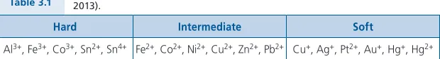
Pearson’s acid-base classification (see Table 3 .1) generalised that the harder metals preferred complexing by harder ligands, both being more ionic, in contrast to the more polarisable and covalent softer metals and ligands . Zinc was inter-mediate, potentially being complexed by either the hydrothermally abundant, harder chloride or hydroxide or maybe the softer bisulphide ligand . An interesting possibility was to explore, at the proper redox and acidity conditions, if there were significant complexes with the dominant sulphur-containing anion, HS- _in

equi-librium with ZnS, in spite of predictions otherwise . Other soft ligands considered included thiosulphate (S2O32-) and polysulphides (Sxy–) .

Table 3.1 Classes of metal complexation behaviour (after Pearson, 1963, 1997; Leach, _2013).

Hard Intermediate Soft

Al3+_{, Fe}3+_{, Co}3+_{, Sn}2+_{, Sn}4+ _Fe2+_{, Co}2+_{, Ni}2+_{, Cu}2+_{, Zn}2+_{, Pb}2+ _Cu+_{, Ag}+_{, Pt}2+_{, Au}+_{, Hg}+_{, Hg}2+

In contrast to inorganic species, only much later in this era were organic compounds also investigated (Landais and Gize, 1997; Seward and Barnes, 1997; Shock et al., 2013) . Nevertheless, Pearson’s correlations suggested that the soft metals would be more readily complexed by HS– _{or S}

2O32– . Following

Consequently, hydrothermal solubilities were measured for the common metals of hydrothermal ores initially at the Geophysical Laboratory of the Carnegie Institution and, after 1960, in an expanded lab at Penn State University . In four years at the Geophysical lab (1956-1960), most measurements were intended to determine the strength of bisulphide complexing although ill-advised detours into solubilities in aqueous polysulphide solutions also were explored . In the absence of any published data on the solubility of metal sulphides in water-immiscible hydrogen polysulphide liquids, I synthesised some first to check for density, colour and refractive index . The second stage, to make solubility measurements in that fluid, was never achieved . At home after a day of polysul-phide fluid testing, a phone call announced that my hood had its glass windows blown out and there was considerable damage to much of the lab . About 300 ml of polysulphide liquid had exploded distributing yellow-green pasty blotches on the walls and left a horrendous stench that was never entirely removed . So, afterwards the lab door was left closed and the windows were open on purpose .

My plan was to experimentally evaluate the complexation constants of the ore metals by working with graduate students and postdocs, ideally astute chemists with polished lab skills

and and comprehension of ore geology . The odyssey began with the Pearson intermediate-class metal, Zn, and measured solu-bilities primarily of sphalerite to investigate the transporting potential of chloride versus bisul-phide complexing (Barnes, 1963) . Later together with Bill Bourcier, we improved the data set for Zn complexes (Bourcier and Barnes, 1987) . Solubility measurements from our Penn State lab also included ore minerals of copper (Crerar and Barnes, 1976), lead (Giordano and Barnes, 1979), silver (Gammons and Barnes, 1989), gold (Shenberger and Barnes, 1989), and mercury (Barnes et al ., 1967; Barnes and Seward, 1997) . At the time, such measurements were not carried out in many labs around the world and the Penn State lab was one of ten which early on produced experimental data on the aqueous complexing

of at least two hydrothermal ore elements . Those labs, listed in Table 3 .2, were located mostly in the United States with others in Canada, Switzerland, Russia, and the United Kingdom .

Table 3.2

Sources of experimental data from laboratories that published on aqueous complexing of multiple ore elements in hydrothermal solutions during the last half of the twentieth century, in alphabetical order.

Institution Principal Scientists

Eidgenössische Technische Hochschule, Zurich T.M. Seward

McGill University, Montreal A.A. Migdisov; A E. William-Jones

Oak Ridge National Laboratory, Tennessee D.A. Palmer; D.J. Wesolowski;

Pennsylvania State University H.L. Barnes; C.W. Burnham

University of California, Riverside F.W. Dickson; G. Tunell

University of Idaho S. Wood

University of Maryland G.A. Helz; G.W. Luther; J.A. Tossell

University of Minnesota W.E. Seyfried

University of Toronto G.M. Anderson; S.D. Scott

University of Wales, Cardiff D. Rickard

Vernadsky Institute, Moscow B.N. Rhyzenko; S. Malinin

Russian Academy of Science IGEM, Moscow A.I. Zotov

Russian Academy of Sciences, Chernogolovka K. Shmulovich

Figure 3.5 Terry Seward.

Note that many of the above complexation

data of Table 3 .3 were products of Terry

Seward’s labs successively in Auckland, New Zealand at the Department of Scien-tific and Industrial Research, then in Zürich, Switzerland at the Eidgenössische Technische Hochschule and now at Victoria University in Wellington, New Zealand . As a migrant from home in

Newfoundland, Canada, Terry has had a

remarkable influence on hydrothermal geochemistry including as my coauthor . We have interacted on several continents, such as when I was presenting a short

course in Sydney, Australia . Di and Terry

invited Mary and me to weekend at their

home in Wellington, New Zealand nomi-nally to consider aspects of a joint publica-tion . On arrival, we had a currency problem . Not having any New Zealand dollars,

gracious host Terry paid our airport tax to export us back to Australia . What

a collaborator!

Just at the end of the 20th _{century and after 5 decades of producing}

hydro-thermal solubility data, a means was found for verifying the behaviour in nature of mineralising solutions with solubilities calculated from well-known complexa-tion constants (Barnes and Rose, 1998) . Thus further testing could be carried out by analysing the contents of single fluid inclusions at each paragenetic stage of ore deposition . The contents of an inclusion could be recovered by laser ablation for analysis by inductively coupled plasma mass spectrometry (LA-ICP-MS) as developed at the Eidgenössische Technische Hochschule (ETH), Zürich (Audétat et al ., 1998) . The saturation state of each mineral at the stage of beginning of precipitation could be compared with the calculated solubility at the precipita-tion temperature . The ETH group found that in an eastern Australia tin deposit, the Yankee Lode, cassiterite deposition began when the measured concentration reached the calculated tin saturation level, a pleasing agreement . The calcu-lated saturation concentration matched the observed, measured concentration at the paragenetic stage where precipitation of cassiterite first began . Similar results with other ore minerals gave reassurance that our chemical modelling was reasonably accurate for understanding the conditions for ore deposition .

contributed significantly to ore transport . For example for zinc, Tagirov and Seward (2010) have found that hydrothermal complexing by chloride is appar-ently dominant over that by the bisulphide ligand except where the salinity of the transporting solution was unusually low . Compilations of newer complexa-tion constants for many metals can be found in Rickard and Luther (2006) and Sherman (2011) .

Table 3.3

Aqueous complexes of interest for hydrothermal transport of metals. These complexes are considered to be predominant in aqueous liquids over other aqueous species, carrying the metals at particular, natural, relatively common combinations of conditions of pH, oxidation state, ligand concentra-tions and temperature.

Metal Complexes References

Ag AgCl₂– _AgCl

32– AgHS0 Ag(HS)2– 1

Au AuCl₂– _AuHS0 _Au(HS)

2¿ 2

Co CoCl₂0 _CoCl

42– CoHS+ 3

Cu+ _CuCl

2– Cu(HS)2– 4

Cu2+ _CuCl+ _CuCl

20 Cu(HS)3–

Fe FeCl+ _FeCl

20 FeHS+ 5

Hg HgCl₂0 _Hg(HS)

20 HgHS2– HgS22– 6

Ni NiCl+ _NiCl

20 NiHS+ 7

Pb PbCl+ _PbCl

20 Pb(HS)3– 8

Sn SnCl+ _SnCl

20 SnCl3– 9

Zn ZnCl+ _ZnCl

20 ZnCl42– Zn(HS)20 Zn(HS)3– 10

1. Stefánson and Seward (2004); Pokrovski et al. (2013)

2. Zotov et al. (1990); Tagirov and Zotov (1996); Vicente et al. (1998); Akinfiev and Zotov (2001); Stefánson and Seward (2004); Tagirov et al. (2006)

3. Migdisov et al. (2011)

4. Etschmann et al. (2010); Sherman (2011)

5. Heinrich and Seward (1990); Rickard and Luther (2006) 6. Barnes and Seward (1997); Rickard and Luther (2006) 7. Rickard and Luther (2006)

8. Giordano and Barnes (1979); Uhler and Helz (1984); Seward and Barnes (1997) 9. Sherman (2011)

10. Bourcier and Barnes (1987); Tagirov and Seward (2010); Mei et al. (2013)

huge memory capacity to calculate accurate quantum mechanical energies and wavefunctions for large atomic clusters (generally termed “ab initio” modelling) began to have an important effect on geosciences in the 1980s (Lasaga, 1998) .

Gerry Gibbs of the Virginia Polytechnic Institute pioneered their use in mineralogy . In the 1990s, Tony Lasaga of Yale University and coworkers intro-duced the application of ab initio calculations to the study of mineral-water inter-actions, atmospheric chemistry and geochemistry (see references in Lasaga, 1998) . These ab initio results and statistical mechanical calculations predict stabili-ties with useful accuracy (Rickard and Luther, 2006; Lemke and Seward, 2008; Sherman, 2011) . Calculated stabilities have been made by faster computers so that the results can now supplant those based directly on solubility measurements, especially where the modelling is confirmed by spectral data .

Advances in spectroscopy are also changing our comprehension of solution characteristics in hydrothermal chemistry . Two changes are especially impor-tant . From Raman spectra (Pokrovski and Dubrovinsky, 2011) and from ab initio modelling calculations (Manning, 2011; Tossel, 2012), there is agreement that the free radical, S₃–_{, at above}

about 250 ºC becomes domi-nant over speciation long assumed to be SO4 2– and H2S

or HS- _.

T h at me a n s t he com mon d iag ra ms for sulphur species distribution with coordinates of log aO₂ –

pHneed to be revised again as suggested by Pokrovski and Dubrovinsky (2011) and shown here in Figure 3 .6 . That change in speciation may correct for calculated Au solubilities involving the older complexes that are well below those observed by fluid inclusion analyses (Kouz-manov and Pokrovski, 2012) . The same is underway with newer Cu+ _{speciation in}

chlo-ride – sulphide solutions that also has been demonstrated by Mei et al . (2013) .

A second discovery of major importance using the new molecular dynamics

tools is that hydrated free aqueous ions and molecules bond into clusters whose dominance affects the kinetics of dissolution and crystallisation (Casey and Swaddle, 2003; Rickard and Luther, 2006; Lemke and Seward, 2008) . Clustering must speed both types of these reactions . Further challenges that molecular modelling should meet are to identify further the speciation of sulphur species to higher temperatures and pressures and the metal complexes associated with them, including with the S3–radical .

Vapour Transport – Another Horizon for the Future

In the above discussions, I emphasised mostly progress made over the last decades on aqueous solubilities . The alternative of gas transport was not consid-ered because vapour pressures of ore minerals up to a few hundred degrees were well known to be very low . So during the 1960s and even later, little credence was given to the possibility of significant vapour transport of the metals into hydro-thermal deposits . The single recognised exception was for mercury vapour . In retrospect, we might as well have undertaken experimental investigations to test the hypothesis that other metals might also be vapour-transported . At that time, our myopic focus was tightly on ore element mobilities in inorganic complexes in aqueous liquids, but to the neglect of both organic and vapour species . Basically, we were busy with our aqueous investigations and neglected vapour transport . Since then, evidence has accumulated early in the 21st _{century that solubilities in}

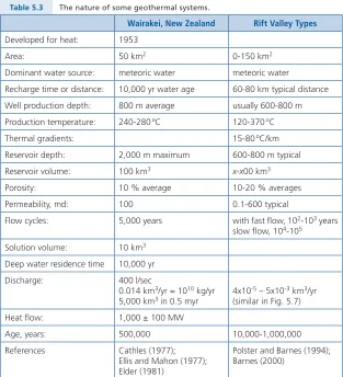
gases are sufficient for important vapour transport not only in mercury deposits but also for epithermal and porphyry copper ores to carry Ag, Au, As, Cu and Mo (see the compilation in Kouzmanov and Pokrovski, 2012) . Noteworthy are recent investigations that favour vapour transport by high vapour solubilities measured in the Tony Williams-Jones laboratory (e.g ., Migdisov and Williams-Jones, 2013; Hurtig and Williams-Jones, 2014a,b; Migdisov et al., 2014) .

Recent analyses of vapour inclusions in quartz (Mavrogenes et al., 2002; Seo and Heinrich, 2013) reveal that both copper and gold had been carried by low density hydrothermal fluids . Experiments with magnetite proved that FeCl2

isgas-soluble enoughto be vapour-transported (Simon et al., 2004), similarly with copper sulphides by Cu(HS)2– (Etschmann et al., 2010) and also with 65Cu

fractionation to be vapour- carried (Rempel et al., 2012) . Active ligands included in ore-forming vapours are found by ab initio calculations to be H3O+, NH4+, and

H3S+ (Lemke and Seward, 2008) . Altogether, the vapour phase now must be

viewed as a fluid capable of hydrothermally transporting important quantities of ore components (Heinrich et al ., 1999) .

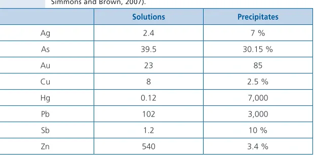
centimetre or less, make it certain that they will be less able solvents but they may act as physical carriers of volatile ore components . Apparent evidence of such transport is seen commonly around volcanic vents, fumaroles, with often vividly coloured coatings of surrounding rocks, i.e. sublimates . In addition to the expected sulphur and arsenic minerals, Pokrovski et al . (2013) report in their compilation appreciable concentrations of Cu, Sn, Mo, Pb, and W in sublimates . However, they conclude that there remain major challenges, both experimental and in modelling, to fully understand vapour transport of ore components, a status comparable to that of liquid solution transport decades ago .

4.

DEDUCING THE CONDITIONS

_{WHERE ORES FORM}

Innovative studies in the 1950s and 1960s that were defining the environ-ments where ores had been deposited, especially those investigating the phase relations and thermodynamic stabilities of ore minerals, were concen-trated in two world centres . Both were in Washington, D .C ., at the U .S . Geological Survey with research led by Paul Barton and Pete Toulmin and at the Geophysical Laboratory of the Carnegie Institution of Washington with research led by Gunnar Kullerud . Their results were often introduced at the evocative, monthly meetings of the Geological Society of Washington and at the daunting, hypercritical sessions of the Geophysical Lab’s Petrologists’ Club . Early progress reports and summaries from the Geophysical Lab were reported in the widely distributed Carnegie Institution’s Annual Reports often long before normal journal publications .

Besides the common use of filling temperatures of fluid inclusions to docu-ment ore deposition temperatures, additional hydrothermal geothermometers were being developed during those early years . There were two special geother-mometers that were of general utility because of the common occurrences of quartz and of sphalerite in hydrothermal deposits . Their development will be followed here because they provided such extensive information for many types of ores, especially for the temperatures of hydrothermal deposition .

How the Geochemistry of Quartz Developed

into the Most Valuable Geothermometer

curve to read an ideal temperature given a measured silica content of an aqueous sample . Nevertheless, non-equilibrium conditions can cause field concentrations to be either lower or higher than the ideal concentrations . The differences can be ascribed to the kinetics of dissolution and of precipitation, which were beginning to be understood .

The study of kinetics in geochemistry began in the 1960s and 1970s (e.g ., see Berner, 1978; Lasaga, 1981, 1998) . Particularly appropriate kinetic data for hydrothermal solutions were the rates for quartz reactions with water but these were not measured until the late 1970s, initially by Don Rimstidt in our Penn State labs (Rimstidt and Barnes, 1980) . Our objective was to use the measurements to model the rates of dissolution and precipitation by considering changes in silica concentrations due to the effects of nature’s heating, cooling, mixing, or boiling . However, precautions were necessary to be certain that the applied rate measure-ments were absolute and not influenced by vagaries in the experimental condi-tions . Ideally, the measurements must be made with quartz particles with the lowest surface energy (equilibrium) so we modified the usual methods to mini-mise the extra surface energy arising from crushing of the material to prepare for our experiments . The more reactive, higher energy surfaces are more soluble and were removed preferentially by dissolution by washing with HF or NaOH solu-tions at ambient temperatures . Alternatively, quartz samples were heated in pure water to roughly 225 ºC for long enough for the silica concentration to become stabilised . Then the solution was quickly vented to prevent any precipitation during subsequent cooling . These three processes gave ideal starting materials with equilibrated quartz surfaces for later dissolution experiments . Since then, there have been many theoretical and experimental studies of the solubility and reaction rates of quartz and of the effects of acidity and alkali concentrations on these rates (Dove, 1994; Rimstidt, 1997; Lasaga, 1998) .

of silica concentrations . These equations have been tested, for example, with data from the Los Azufres geothermal field that revealed an accuracy of ±18 ºC at 240 – 300 ºC (Verma, 2012) .

The ideal silica solubility curve is based on equilibration with quartz as a stable solid with no excess energy contributions from textural or structural states or disequilibrium processes . Geothermal systems often have other silica phases contributing to their hydrothermal concentrations, such as the silica glass or cristobalite of volcanics, or previously precipitated amorphous silica or chal-cedony (mix of quartz plus moganite), each of which have higher solubilities than quartz . Consequently, these other silica phases may dissolve to raise the silica concentration above that of quartz causing an anomalously high apparent crystallisation temperature . In fact, comparison of quartz-based temperatures with directly measured geothermal temperatures below about 150 ºC have, not uncommonly, shown such apparently inaccurate temperatures . Corrections can be made for equilibrium with specific silica minerals by using reference solu-bility – temperature equations that are available for both chalcedony and amor-phous silica (Karingithi, 2000) . Also, there are some rate data from our lab for dissolution and precipitation of cristobalite over the useful range of 150 – 300 ºC (Renders et al ., 1995) . These rate data can be used for modelling of cristobalite geothermometry just as has been done for quartz .

Don Rimstidt and I modelled the representative behaviour of the quartz geothermometer along the P-T, liquid – vapour curve of water as shown in Figure 4 .1 (Rimstidt and Barnes, 1980) . We selected fluid ascension rates to be along typical gradients like those of the 3 x 10-5 _{m/sec at El Tatio, Chile . The ratio}

of A/M (reactive area in m2_{/mass of solution in kg) that is assumed at 100 m}2_/kg

is equivalent to the textures of a very fine grained sediment; comparatively a vein 0 .1 mm wide would have an A/M of 20 m2_{/kg .}

Figure 4.1 The effect of the ascent rate on the quartz geothermometer temperature. Assumed are a geothermal gradient of 138 ºC/km and an A/M of 100 m2_/kg