Intelligent control of biped robots: optimal fuzzy tracking control via multi-objective particle swarm optimization and genetic algorithms

(1)

AUT Journal of Mechanical Engineering

AUT J. Mech. Eng., 4(2) (2020) 183-192 DOI: 10.22060/ajme.2019.16171.5808

Intelligent Control of Biped Robots: Optimal Fuzzy Tracking Control via

Multi-Objective Particle Swarm Optimization and Genetic Algorithms

M.J. Mahmoodabadi1_{*, M. Taherkhorsandi}2

1_{Department of Mechanical Engineering, Sirjan University of Technology, Sirjan, Iran.}

2_{Department of Mechanical Engineering, University of Texas at San Antonio, San Antonio, USA.}

ABSTRACT: This paper is concerned with fuzzy tracking control optimized via multi-objective particle swarm optimization for stable walking of biped robots. To present an optimal control approach, multi-objective particle swarm optimization is used to design the parameters of the control method in comparison to three effectual multi-objective optimization algorithms in the literature. In particle swarm optimization, a dynamic elimination technique is utilized as a novel approach to prune the archive effectively. Moreover, a turbulence operator is used to skip the local optima and the personal best position of each particle is determined by making use of the Sigma method. Normalized summation of angles errors and normalized summation of control efforts are two conflicting objective functions addressed by dint of multi-objective optimization algorithms in the present investigation. By contrasting the Pareto front of multi-objective particle swarm optimization with the Pareto fronts of other methods, it is illustrated that multi-objective particle swarm optimization performs with high accuracy, convergence and diversity of solutions in the design of fuzzy tracking control for nonlinear dynamics of biped robots. Finally, the proper performance of the proposed controller is demonstrated by the results presenting an appropriate tracking system and optimal control inputs. Indeed, the appropriate tracking system and optimal control inputs prove the efficiency of optimal fuzzy tracking control in dealing with the nonlinear dynamics of biped robots.

Review History: Received: 24 Apr. 2019 Revised: 25 Jul. 2019 Accepted: 22 Sep. 2019 Available Online: 4 Oct. 2019

Keywords:

Fuzzy tracking control Multi-objective optimization Particle swarm optimization Genetic algorithm optimization Biped robots.

183 1. Introduction

1.1 Definition and importance of subject

Of particular interest are biped robots which are the most similar robot to humans and are capable of doing formidable and difficult tasks. Due to their heavy nonlinear dynamic equations, implementing an appropriate controller capable of providing the stability of biped robots is a challenging subject and has attracted a great deal of researchers’ interest. Population-based paradigms to solve constrained optimization problems are of considerable interest to researchers owing to their simple structure, easy implementation and fast computation. Swarm-based and genetic-based paradigms are two prominent population-based heuristic algorithms to address constrained optimization problems [1]. Particle Swarm Optimization (PSO) is a swarm intelligence method emulating the behavior of social species such as flocking birds, swimming wasps, schooling fish, etc. On the other hand, genetic algorithm optimization is a traditional optimization technique inspired by natural evolution, such as inheritance, mutation, selection, and crossover. Fuzzy control, which is straightforward conceptually, can be regarded as an effective control approach in dealing with complex nonlinear systems. Due its unique advantages, it has been utilized extensively in

a broad range of subjects, to name but a few, aviation industry [2-4], robotics [5-7], vehicles [8-10], and turbines [11-13].

1.2 Explanation of references

Particularly, Li et al. [14] proposed two efficient fuzzy control methods, i.e. a fuzzy feedback control method and an adaptive fuzzy control method to suppress the state variables of the Lorenz-Stenflo chaotic system to its equilibrium point. Yeh et al. [15] introduced a scheme of neural-network fuzzy control for a time-delay chaotic building system by dint of the Tagaki-Sugeno fuzzy model and parallel distributed compensation scheme in the controller design. Chen[16] developed an easy-to-use fuzzy control approach for interconnected structural systems and guaranteed the stability of the control approach by using the fuzzy Lyapunov functions. Li et al. [17] presented the adaptive fuzzy robust control problem for a class of Single-Input and Single-Output (SISO) stochastic nonlinear systems in a strict-feedback form and guaranteed that the closed-loop system is input-state-practically stable and the output of the system converges to a small neighborhood of the origin by appropriately tuning several design parameters. Wang et al. [18] proposed a novel adaptive fuzzy controller to implement non-overshoot control in power plants where the Lyapunov-based adaptive law was utilized to guarantee the stability of the controller and

*Corresponding author’s email:[email protected]

(2)

M.J. Mahmoodabadi and M. Taherkhorsandi, Amirkabir J. Mech. Eng., 4(2) (2020) 183-19292, DOI: 10.22060/ajme.2019.16171.5808

184 a modified adaptive binary harmony search algorithm was used to search the optimal control parameters of the control approach.

Effective control approaches have been successfully proposed and implemented in the literature regarding biped robots as follows, to name but a few, fuzzy motion control based on reinforcement learning and Lagrange polynomial interpolation [19], a dynamic balance control involving Kalman filter and the fuzzy motion controller [20], a feedback-control law obtained via feedback-linearization techniques [21], a structure of robust adaptive control involving balancing and posture control for regulating the center-of-mass position and trunk orientation of biped robots [22], adaptive walking control inspired by the biological concept of central pattern generators [23], a robust adaptive sliding-mode control scheme based on the fuzzy wavelet neural network for a class of condenser-cleaning mobile manipulator regarding parametric uncertainties and external disturbances [24], and a time-sequence-based fuzzy Support Vector Machine (SVM) learning control system considering time properties of biped walking samples [25].

In this paper, particle swarm optimization in comparison to genetic algorithm optimization is used to ascertain the optimal parameters of the fuzzy control approach. Since these optimization algorithms benefit from unique advantages, they have been widely employed to ascertain optimal solutions in the research domain of control, specifically, predictive model control [26-29], sliding mode control [30-32], robust control [33-36] and fuzzy control [37-40]. Soltanpour and Khooban[41] utilized particle swarm optimization to find the existing membership functions of fuzzy sliding mode control for the position of a robot manipulator. Wonohadidjojo et al. [42] used a fuzzy logic controller based upon particle swarm optimization for the position control of an electro-hydraulic actuator system and reduced the chattering problem significantly. Niknam et al. [43] introduced an optimal type-2 fuzzy sliding mode controller by means of a novel heuristic algorithm, i.e. particle swarm optimization with random inertia weight and applied it to an inverted pendulum system. Schacher [44] constructed an optimal feedback controller for robots concerning stochastic uncertainties in the initial conditions with expected cost functions evaluating the primary control expenses and the tracking error. Bui et al. [45] designed three controllers involving optimal fuzzy control using hedge algebras, fuzzy control using hedge algebras and conventional fuzzy control in order to provide the stability in the vertical position of a damped-elastic-jointed inverted pendulum subjected to a time-periodic follower force. Chaouch et al. [46] proposed a self-tuning fuzzy inference sliding mode control approach optimized online based upon the Takagi-Sygeno type of rules and a back-propagation algorithm to minimize a cost function for single inverted pendulum position tracking control.

1.3 Illustration of the new work compared with previous works

This study is in advance of authors’ previous studies on

optimal control approaches as follows. While sliding mode tracking control applied to a biped robot [47] and decoupled sliding mode control implemented in an inverted pendulum system [48] were studied in the literature, fuzzy tracking control with appropriate membership functions and error indexes is presented and studied in this paper as an effectual and straightforward controller not involving the intricacies and disadvantages of sliding mode control, e.g. the chattering problem of control inputs. To this end, the rest of this paper is organized as follows. Section 2 provides the dynamic equations and modeling of the biped robot in the lateral plane. The architecture and formulation of fuzzy tracking control for the biped robot is presented in Section 3. Section 4 involves the details of multi-objective particle swarm optimization and a dynamic elimination technique used to prune the archive effectively. Section 5 includes the results and analysis of proposed optimal fuzzy tracking control for the biped robot. Conclusions are provided in Section 6.

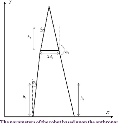
2. The Dynamics and Modeling of the Biped Robot The biped robot walking in the lateral plane is modeled by means of a three-link model according Fig. 1 [47]. The first link is the stance leg on the ground, the second link represents the head, arms, and trunk, and the third link is the swing leg. More precisely, these links move freely in the lateral plane. The parameters of the biped robot are acquired from the anthropometric table for a humanoid robot having 171 cm height and 74 kg weight and are presented in Table 1 [47].

The distance between two legs of the model ( 2d₂) equals 32.7

cm.

In order to gain the dynamic equations of the biped robot, the Newton-Euler approach is used to derive the dynamic

equations of the model [47]. Moreover, θ₁,θ₂ and θ₃ are

the angles between the first, second and third links and the assumed vertical line of these links, respectively. Thus, the dynamic equations of the model for θ₁,θ₂ and θ₃ are:

Fig. 1. The parameters of the robot based upon the anthropometric table.

Fig. 1. The parameters of the robot based upon the anthropometric table.

(3)

185

where, θ_pd₍_p_{=1,2,3) are the desired values of joint angles}

θ_p (p=1,2,3). Moreover, θ_pd₍_q_{=1,2,3) are the derivative of} the desired values of joint angular velocities θ_p (p=1,2,3). Further, E_p and E_q illustrate the related errors to the joint angles and angular velocities, respectively. In order to have the normalized errors, new error indexes parameters are introduced as follows.

Then, a membership function is constructed by Fig. 2 and it is illustrated in Table 2. In Fig. 2, the reference result of the consequent variable should be calculated by the product-sum gravity method [49,50]. Finally, the control efforts are obtained by Eq. (6).

where, θ₁,θ₂ and θ₃are the joint angles, u₁,u₂and u₃ are the control inputs, m₁,m₂and m₃ are the masses of the links,

l₁, l₂and l₃ are the lengths of the links, and 2d₂ is the distance between two legs.

3. Fuzzy Tracking Control of the Biped Robot

The proposed fuzzy tracking control is based upon a closed-loop fuzzy system. The stages of the control method are designed and constructed step by step as follows. To control the system, the state variable vector is chosen as . Moreover, the errors could be defined as Eq. (4):

Table 1. The Anthropometric parameters of the model of the biped robot. Table 1. The Anthropometric parameters of the model of the biped robot. The characteristics of the robot First link Second link Third link

Mass 𝑚𝑚1= 13.75 𝑚𝑚2= 46.5 𝑚𝑚3= 13.75

Inertia 𝐼𝐼1= 1.4 𝐼𝐼2= 3.25 𝐼𝐼3= 1.4

Length 𝑙𝑙1= 0.91 𝑙𝑙2= 0.8 𝑙𝑙3= 0.91

The center of gravity ℎ1= 0.50 ℎ2= 0.27 ℎ3= 0.50

Table 2. The rule modules for each input item.

𝑥𝑥𝑖𝑖 (𝑖𝑖 = 1,2,3,4,5,6)

Antecedent Variables Consequent Variables 𝑓𝑓𝑖𝑖(𝑖𝑖 = 1,2,3,4,5,6)

Negative Big −1.0

Zero 0.0

Positive Big 1.0

Table 3. The objective functions and design variables corresponding to the optimum design points A, B, and C.

Optimum design points A B C

Normalized summation of angles errors 2.340 × 10−1 _{3.159 × 10}−1 _{6.269 × 10}−1

Normalized summation of control efforts 4.762 × 10−1 _{1.727 × 10}−1 _{8.012 × 10}−2

Design variable 𝑤𝑤1 1.998 × 103 1.999 × 103 1.984 × 103

Table B

Equations typed in MathType Equation

number

1 1 1 2 1 1 1

1 1 2 3 1 1 1 1 1 2

11 2 2 2 1

2

2 2 1 2 2 2 1

2 2 1

1 3 11 2 2 2 1

3 2 3 3 1

2 2

sin

sin ( ) ( )

{ sin( )

cos( )} { cos( )

sin( )}

[ {2 sin( )

( )cos( )

2

I u u h m g

l g m m h m h l m

l d

h d

h

l m l d

l h d                                                           2

2cos(21)3 3(l h3)sin(31)]

1

2 2 2 3 2 2 2

2 2 2 3 2 2

2 1 2 2 1

1 2 1 3 2 1

2 1 2 2 1 2

1 1 2 2 1 2

2 1 3 2 1 2 1 2 2 1

2 2 2

2 2 2 3 2 2 2

cos

sin 2 cos

cos( )

sin( ) 2

sin( )

[sin( )

cos( )2 cos( ) ]

[ 4 ]

I u u m d g

m h g m d g

m h l m d l m d l m l h

m d l m d l

m d m d m h

                                _  _               

 3 3 2 3 3 2 3

2

3 3 2 3 3 2 3

[2 ( )sin( )]

[2 ( )cos( )]

m d l h m d l h

 

  

  

 

2

3 3 3 3 3 3 3 3 3 3 1 3 1 1

2 3 3 3 1 1 3 1

2 3 3 3 2 3 2 2 3 3 3 3 2 2

2 3 3 3 3

( ) sin

( ) cos( )

( ) sin( )

2 ( )sin( )

2 ( )cos( )

( )

I l h m g u

m l h l m l h l d m l h d m l h m l h

                                3 4 1,2,3 d

p p p

E   p

1,2,3

d

q q q

E   q

(1)

Table B

number

1 1 1 2 1 1 1

1 1 2 3 1 1 1 1 1 2

11 2 2 2 1

2

2 2 1 2 2 2 1

2 2 1

1 3 11 2 2 2 1

3 2 3 3 1

2 2

sin

sin ( ) ( )

{ sin( )

cos( )} { cos( )

sin( )}

[ {2 sin( )

( )cos( )

2

I u u h m g

l g m m h m h l m

l d

h d

h

l m l d

l h d                                                           2

2cos(21)3 3(l h3)sin(31)]

1

2 2 2 3 2 2 2

2 2 2 3 2 2

2 1 2 2 1

1 2 1 3 2 1

2 1 2 2 1 2

1 1 2 2 1 2

2 1 3 2 1 2 1 2 2 1

2 2 2

2 2 2 3 2 2 2

cos

sin 2 cos

cos( )

sin( ) 2

sin( )

[sin( )

cos( )2 cos( ) ]

[ 4 ]

I u u m d g

m h g m d g

m h l m d l m d l m l h

m d l m d l

m d m d m h

                                _  _               

 ₃ _{3 2 3} ₃ ₂ ₃

2

3 3 2 3 3 2 3

[2 ( )sin( )]

[2 ( )cos( )]

m d l h m d l h

 

  

  

 

2

3 3 3 3 3 3 3 3 3 3 1 3 1 1

2 3 3 3 1 1 3 1

2 3 3 3 2 3 2 2 3 3 3 3 2 2

2 3 3 3 3

( ) sin

( ) cos( )

( ) sin( )

2 ( )sin( )

2 ( )cos( )

( )

I l h m g u

                                3 4 1,2,3 d

p p p

E   p

1,2,3

d

q q q

E   q

(2)

Table B

number

1 1 1 2 1 1 1

1 1 2 3 1 1 1 1 1 2 11 2 2 2 1

2

2 2 1 2 2 2 1

2 2 1

1 3 11 2 2 2 1

3 2 3 3 1

2 2

sin

sin ( ) ( )

{ sin( )

cos( )} { cos( )

sin( )}

[ {2 sin( )

( )cos( )

2

I u u h m g

l g m m h m h l m

l d

h d

h

l m l d

l h d                                             _              2

2cos(21)3 3(l h3)sin(31)] 1

2 2 2 3 2 2 2

2 2 2 3 2 2

2 1 2 2 1

1 2 1 3 2 1

2 1 2 2 1 2

1 1 2 2 1 2

2 1 3 2 1 2 1 2 2 1

2 2 2

2 2 2 3 2 2 2

cos

sin 2 cos

cos( )

sin( ) 2

sin( )

[sin( )

cos( )2 cos( ) ]

[ 4 ]

I u u m d g

m h g m d g

m h l m d l m d l m l h

m d l m d l

m d m d m h



 



 



 



            _  _               

 ₃ _{3 2 3} ₃ ₂ ₃

2

3 3 2 3 3 2 3

[2 ( )sin( )]

[2 ( )cos( )]

m d l h m d l h

 



 

  

 

2

3 3 3 3 3 3 3

3 3 3 1 3 1 1 2 3 3 3 1 1 3 1

2 3 3 3 2 3 2 2 3 3 3 3 2 2

2 3 3 3 3

( ) sin

( ) cos( )

( ) sin( )

2 ( )sin( )

2 ( )cos( )

( )

I l h m g u

                                3 4 1,2,3 d

p p p

E   p

1,2,3

d

q q q

E   q

(3)

Table B

number

1 1 1 2 1 1 1

1 1 2 3 1 1 1 1 1 2

11 2 2 2 1

2

2 2 1 2 2 2 1

2 2 1

1 3 11 2 2 2 1

3 2 3 3 1

2 2

sin

sin ( ) ( )

{ sin( )

cos( )} { cos( ) sin( )}

[ {2 sin( ) ( )cos( )

2

I u u h m g

l g m m h m h l m

l d

h d

h

l m l d

l h d                                             _              2

2cos(21)3 3(l h3)sin(31)] 1

2 2 2 3 2 2 2

2 2 2 3 2 2

2 1 2 2 1 1 2 1 3 2 1

2 1 2 2 1 2

1 1 2 2 1 2

2 1 3 2 1 2 1 2 2 1

2 2 2

2 2 2 3 2 2 2

cos

sin 2 cos

cos( )

sin( ) 2

sin( )

[sin( )

cos( )2 cos( ) ]

[ 4 ]

I u u m d g m h g m d g m h l m d l m d l m l h

m d l m d l m d m d m h

                                _  _               

 3 3 2 3 3 2 3 2

3 3 2 3 3 2 3

[2 ( )sin( )]

[2 ( )cos( )]

m d l h m d l h

 

  

  

 

2

3 3 3 3 3 3 3

3 3 3 1 3 1 1 2 3 3 3 1 1 3 1

2 3 3 3 2 3 2 2 3 3 3 3 2 2

2 3 3 3 3

( ) sin ( ) cos( ) ( ) sin( ) 2 ( )sin( ) 2 ( )cos( )

( )

I l h m g u

                                3 4 1,2,3 d

p p p

E   p

1,2,3

d

q q q

E   q

(4)

Equations typed in MathType Equation number 5 2 2 1 1 1 w f w f

u  

4 4 3 3 2 w f w f

u  

6 6 5 5

3 w f w f

u  

6 ) 1 ( ) ( ) 1 (       t v t x t

xi i i

7

1 1

2 2

( 1) ( ) ( ( ))

( ( ))

i

pbest

i i i

gbest _i

v t W v t C r x x t

C r x x t

            8                        else t fix t if iteration maximum t Dynamic 0 10 10 100  9 / (| | | |) ( ) / (| | | |) d

Ep p p p

d d

p p p p

Index E  

         / (| | | |) ( ) / (| | | |) d

Eq q q q

d d

q q q q

Index E  

   

  

 

(5)

Fig. 1. The parameters of the robot based upon the anthropometric table.

Fig. 2. The membership function for fuzzy control of the biped robot. Fig. 2. The membership function for fuzzy control of the biped

robot.

Table 2. The rule modules for each input item.

Table 1. The Anthropometric parameters of the model of the biped robot.

The characteristics of the robot First link Second link Third link Mass 𝑚𝑚1= 13.75 𝑚𝑚2= 46.5 𝑚𝑚3= 13.75

Inertia 𝐼𝐼1= 1.4 𝐼𝐼2= 3.25 𝐼𝐼3= 1.4

Length _𝑙𝑙₁_{= 0.91} 𝑙𝑙2= 0.8 𝑙𝑙3= 0.91

Table 2. The rule modules for each input item.

𝑥𝑥𝑖𝑖 (𝑖𝑖 = 1,2,3,4,5,6)

Antecedent Variables Consequent Variables 𝑓𝑓𝑖𝑖(𝑖𝑖 = 1,2,3,4,5,6) Negative Big −1.0

Zero 0.0

Positive Big 1.0

Table 3. The objective functions and design variables corresponding to the optimum design points A, B, and C. Optimum design points A B C

Normalized summation of control efforts _{4.762 × 10}−1 _{1.727 × 10}−1 _{8.012 × 10}−2

Equations typed in MathType Equation number 5 2 2 1 1

1

w

f

w

f

u





4 4 3 3

2 w f w f

u  

6 6 5 5

3 w f w f

u  

6

)

1 (

)

(

)

1 (















t

v

t

x

t

x

_i _i _i

7

1 1

2 2

( 1)

( )

(

( ))

(

( ))

i

pbest

i i i

gbest _i

v t

W v t C r x

x t

C r x

x t

     

 









8











































else

t

fix

t

if

iteration

maximum

t

Dynamic

0

10

100 

9

/ (|

| | |)

(

) / (|

| | |)

d

Ep p p p

d d

p p p p

Index

E













/ (|

| | |)

(

) / (|

| | |)

d

Eq q q q

d d

q q q q

Index

E













(4)

186 In Eq. (6), w₁, w₂, w₃, w₄, w₅ and w₆ are weight constants and these parameters are usually identified by a trial-and-error process. One proper approach to choose these factors is to use multi-objective optimization algorithms such as particle swarm optimization, genetic algorithm optimization, etc. In this paper, multi-objective particle swarm optimization is utilized to eliminate the boring and repetitive trial-and-error process and find parameters w_i (i=1,2,3,4,5,6) of fuzzy control.

4. Multi-Objective Particle Swarm Optimization

Particle swarm optimization is a swarm intelligence method emulating the behavior of social species such as flocking birds, swimming wasps, schooling fish, etc. It is a population-based paradigm to address constrained optimization problems. In PSO, each candidate solution is associated with a velocity. The candidate solutions are named particles and the position of each particle changes according to its own experience and that of its neighbors (velocity). It is expected that the particles will move toward better solution areas. The particles are manipulated as follows.

where, xi(t)

→

is the position of particle i and vi(t)

→

represents the velocity of particle at time step t. r1,r2∈[01,] are random values. C₁ is the cognitive learning factor and C₂

is the social learning factor. W is the inertia weight which

is employed to balance the global and local search ability.

C₁ , C₂ and W are obtained by the formulas presented in

reference [47]. The personal best position of the particle i is

i pbest

x

→

and xgbest

→

is the position of the best particle of the entire

swarm. By regarding a large value of C₁ and a small value

of C₂, particles are allowed to move around their personal

best position (xgbest

→

). However, by regarding a small value of C₁ and a large value of C₂, particles converge to the best particle of the entire swarm (xgbest

→

). A large inertia weight makes a global search straightforward while a small inertia weight makes a local search easy. The strategies to choose the global best position and the personal best position, i.e.

gbest

x

→

and xpbesti →

are presented in reference [47]. Moreover, the turbulence operator is utilized to escape a local minimum and have the opportunity to ascertain superior positions [47].

In the multi-objective optimization problems, an archive is used to store the set of dominated solutions. If all the non-dominated solutions are stored in the archive, the size of the

archive enhances very quickly. The archive must be updated at the each iteration. If the size of the archive expands too much, this update may become computationally expensive. To address this issue, a criterion is needed to diminish the growth of the archive [51-54]. We previously proposed adaptive ε_elimination to retain more leaders in the archive in the initial iterations and this increases the convergence of the PSO algorithm [47]. Here, a dynamic elimination technique is used to prune the archive. In this approach, each particle in the archive has an elimination radius equaling εDynamic and

if the Euclidean distance (in the objective function space) between two particles is fewer than εDynamic , then one of them

will be omitted. Fig. 3 illustrates this technique as an example in a two-objective function space.

In this study, the following equation is employed to determine the value of εDynamic:

where, t is the current iteration number. The maximum

iteration is the maximum number of allowable iterations, and

1 wf w f

u  

4 4 3 3

2 wf wf

u  

6 6 5 5

3 wf w f

u  

6 ) 1 ( ) ( ) 1 (      t v t x t

xi i i

7

1 1

2 2

( 1) ( ) ( ( ))

( ( ))

i

pbest

i i i

gbest i

v t W v t C r x x t C r x x t

            8                        else t fix t if iteration maximumt Dynamic 0 10 10 100  9 / (| | | |) ( ) / (| | | |) d Ep p p p d d p p p p

Index E  

         / (| | | |) ( ) / (| | | |) d Eq q q q d d q q q q

Index E  

   

  

 

is a function that rounds

1 wf wf

u  

4 4 3 3

2 wf w f

u  

6 6 5 5

3 wf wf

u  

6 ) 1 ( ) ( ) 1 (     t v t x t

xi i i

7

1 1

2 2

( 1) ( ) ( ( ))

( ( ))

i

pbest

i i i

gbest i

v t W v t C r x x t C r x x t

            8                        else t fix t if iteration maximumt Dynamic 0 10 10 100  9 / (| | | |) ( ) / (| | | |) d Ep p p p d d p p p p

Index E  

         / (| | | |) ( ) / (| | | |) d Eq q q q d d q q q q

Index E  

   

  

 

to the nearest integer in

the direction of zero.

Using Eq. (9) for εDynamic leads to retain more

non-dominated solutions in the archive at the initial iterations (the elimination radius is small) and this enhances the convergence of the algorithm. When the current iteration grows, the

Equations typed in MathType Equation number 5 2 2 1 1 1 wf w f

u  

4 4 3 3

2 w f w f

u  

6 6 5 5

3 w f w f

u  

6 ) 1 ( ) ( ) 1 (       t v t x t

xi i i

7

1 1

2 2

( 1) ( ) ( ( ))

( ( ))

i pbest

i i i

gbest _i

C r x x t

Ep p p p

d d

p p p p

Index E  

         / (| | | |) ( ) / (| | | |) d

Eq q q q

d d

q q q q

Index E  

   

  

 

(7)

u  

4 4 3 3

2 w f w f

u  

6 6 5 5

3 w f w f

u  

6 ) 1 ( ) ( ) 1 (       t v t x t

xi i i

7

1 1

2 2

( 1) ( ) ( ( ))

( ( ))

i pbest

i i i

gbest _i

C r x x t

Ep p p p

d d

p p p p

Index E  

         / (| | | |) ( ) / (| | | |) d

Eq q q q

d d

q q q q

Index E  

   

  

 

(8)

u  

4 4 3 3 2 w f w f

u  

6 6 5 5 3 w f w f

u  

6 ) 1 ( ) ( ) 1 (      t v t x t

xi i i

7

1 1 2 2

( 1) ( ) ( ( )) ( ( ))

i pbest

i i i

gbest _i

C r x x t

Ep p p p

d d

p p p p

Index E  

         / (| | | |) ( ) / (| | | |) d

Eq q q q

d d

q q q q

Index E  

   

  

 

(9)

Fig. 3. The particles located in the radius of other particles will be removed using the εDynamic technique.

Fig. 3.The particles located in the radius of other particles will be removed using the



_Dynamic technique.

Fig. 4. The changes of



_Dynamic over iterations.

5 10 15 20 25 30 35 40 45 50

0 0.5 1 1.5 2 2.5 3 3.5 4 4.5

5 x 10 -3

t

Dyn

am

(5)

187 elimination radius would be large and more similar solutions will be removed. This increases the speed of the algorithm and uniform diversity of non-dominated solutions. Fig. 4 shows the changes of εDynamic over iterations.

5. Pareto Design of the Proposed Fuzzy Tracking Control In fuzzy tracking control, the heuristic fuzzy parameters

w_i (i=1,2,3,4,5,6) must be ascertained by means of an

approach providing appropriate control performance. In this respect, multi-objective particle swarm optimization is used to determine the proper parameters and eliminate the tedious and repetitive trial-and-error process. The performance of a controlled closed loop system is usually evaluated by a variety of goals. In this paper, the normalized summation of angles errors and normalized summation of control efforts are regarded as the objective functions. These objective functions

have to be minimized simultaneously. The vector [w₁ w₂

w₃ w₄ w₅ w₆] is the vector of selective parameters of fuzzy mode control and all the elements of the vector are positive constants. The normalized summation of angles errors and normalized summation of control efforts are functions of this vector’s components. This means that by selecting various values for the selective parameters, we can make changes in the normalized summation of angles errors and normalized summation of control efforts. The regions of the selective parameters are:

1000<w1<2000, 100<w2<500, 100<w3<1000,

10<w4<100, 1000<w5<2000, 100<w6<500

When solving the multi-objective problem, the population

size is set at 30 and also, the maximum iteration is set at

150. The parameters of the multi-objective algorithm are

chosen as follows. The inertia weight W₁=0.9 and W₂=0.4;

C₁ is linearly decreased with C_1i=2.5 and C_1f=0.5; and

C₂ is linearly increased with C_2i=0.5 and C_2f=2.5, over

iteration. The neighborhood radius of the leader selection is R_neighborhood=0.02. The Pareto front of this multi-objective problem is shown in Fig. 5. Furthermore, the feasibility and efficiency of multi-objective particle swarm optimization is

assessed in comparison with Sigma method by Mostaghim and Teich [52], modified NSGAII by Atashkari et al. [55] and MATLAB Toolbox MOGA.

While the performances of these algorithms are appropriate for this problem, multi-objective particle swarm optimization has more uniformity and diversity in comparison to other algorithms. Points A and C in Fig. 5 denote the best normalized summation of angles errors and normalized summation of control efforts, correspondingly. All the points of the Pareto front are non-dominated and can be selected by designers based upon the design criteria. Point C in Fig. 5 is the trade-off optimum choice when considering the minimum values of both of the normalized summation of angles errors and normalized summation of control efforts. Objective functions and design variables corresponding to the optimum design points A, B, and C are shown in Table 3. The real

Fig. 3.The particles located in the radius of other particles will be removed using the



_Dynamic technique.

Fig. 4. The changes of



_Dynamic over iterations.

5 10 15 20 25 30 35 40 45 50

0 0.5 1 1.5 2 2.5 3 3.5 4 4.5

5 x 10 -3

t

Dyn

am

ic

Fig. 4. The changes of εDynamic technique.

Fig. 5. The Pareto fronts of multi-objective particle swarm optimization, Sigma method [58], modified NSGAII [57], MATLAB Toolbox for the optimal control design of the biped

robot.

Fig. 5. The Pareto fronts of multi-objective particle swarm optimization, Sigma method [58], modified NSGAII [57], MATLAB Toolbox for the optimal control design of the biped robot.

0.2 0.25 0.3 0.35 0.4 0.45 0.5 0.55 0.6 0.65 0.05

0.1 0.15 0.2 0.25 0.3 0.35 0.4 0.45 0.5 0.55

Normalized summation of angles errors

N

or

m

al

iz

ed s

um

m

at

ion of

c

ont

rol

e

ffor

ts

MATLAB Toolbox Modified NSGAII Sigma method Proposed method A

B

(6)

188 tracking trajectories of the optimum design points A, B, and C are shown in Figs. 6 to 8. As it is illustrated in Figs. 9 to 11, the design point C has the minimum control effort among the

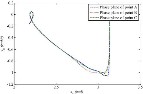
optimum design points and point A has the maximum effort. Moreover, the phase plane diagrams of fuzzy tracking control are presented in Figs. 12 to 14.

Table 1. The Anthropometric parameters of the model of the biped robot. The characteristics of the robot First link Second link Third link

Mass 𝑚𝑚1= 13.75 𝑚𝑚2= 46.5 𝑚𝑚3= 13.75

Inertia 𝐼𝐼1= 1.4 𝐼𝐼2= 3.25 𝐼𝐼3= 1.4

Length 𝑙𝑙1= 0.91 𝑙𝑙2= 0.8 𝑙𝑙3= 0.91

Table 2. The rule modules for each input item. 𝑥𝑥𝑖𝑖 (𝑖𝑖 = 1,2,3,4,5,6)

Antecedent Variables Consequent Variables 𝑓𝑓𝑖𝑖(𝑖𝑖 = 1,2,3,4,5,6) Negative Big −1.0

Zero 0.0

Positive Big 1.0

Table 3. The objective functions and design variables corresponding to the optimum design points A, B, and C.

Optimum design points A B C

Normalized summation of control efforts 4.762 × 10−1 _{1.727 × 10}−1 _{8.012 × 10}−2

Table 3. The objective functions and design variables corresponding to the optimum design points A, B, and C.

Fig. 6. Trajectory tracking θ1 of the optimum design points A, B, and C shown in the Pareto front.

لودج

خ

:

تاحلاصا

زا یتساوخرد

ناگدنسیون

)یسیلگنا هلاقم(

Corrections made

Paragraph/Figure/Table

number

Page

number

Item

figure 6

6

1 figure 7

6

2

0 0.5 1 1.5 2 2.5 3 3.5 4

-0.2 -0.15 -0.1 -0.05 0

Time (s)  1

(ra

d)

Trajectory tracking of point A Trajectory tracking of point B Trajectory tracking of point C Desired trajectory

0 0.5 1 1.5 2 2.5 3 3.5 4

0 0.05 0.1 0.15 0.2 0.25

Time (s)  (ra 2

d)

1.55 1.56 1.57 1.58 1.59 1.6 1.61 -0.1907

-0.1906 -0.1905 -0.1904 -0.1903

Fig. 7. Trajectory tracking θ₂ of the optimum design points A, B, and C shown in the Pareto front.

لودج

خ

:

تاحلاصا

زا یتساوخرد

ناگدنسیون

)یسیلگنا هلاقم(

Corrections made

Paragraph/Figure/Table

number

Page

number

Item

figure 6

6

1 figure 7

6

2

0 0.5 1 1.5 2 2.5 3 3.5 4

-0.2 -0.15 -0.1 -0.05 0

Time (s)  (ra1

d)

0 0.5 1 1.5 2 2.5 3 3.5 4

0 0.05 0.1 0.15 0.2 0.25

Time (s)  (ra2

d)

1.55 1.56 1.57 1.58 1.59 1.6 1.61 -0.1907

(7)

189 Fig. 9. Control effort u1 for the optimum design points A, B, and

C shown in the Pareto front.

Corrections made Paragraph/Figure/Table

number Page

number Item

figure 8 7

3

figure 9 7

4

0 0.5 1 1.5 2 2.5 3 3.5 4

2 2.2 2.4 2.6 2.8 3 3.2 3.4

Time (s)

 (ra3

d)

0 0.5 1 1.5 2 2.5 3 3.5 4

-500 -400 -300 -200 -100 0 100

Time (s) u1

(N

.m

)

Control effort of point A Control effort of point B Control effort of point C 3.25 3.3 3.35 3.4 3.45 3.5 3.55 3.6 3.65

2.19 2.2 2.21 2.22 2.23 2.24

Fig. 8. Trajectory tracking θ3 of the optimum design points A, B, and C shown in the Pareto front.

number Page

number Item

figure 8 7

3

figure 9 7

4

0 0.5 1 1.5 2 2.5 3 3.5 4

2 2.2 2.4 2.6 2.8 3 3.2 3.4

Time (s)

 (ra3

d)

0 0.5 1 1.5 2 2.5 3 3.5 4

-500 -400 -300 -200 -100 0 100

Time (s) u1

(N

.m

)

Control effort of point A Control effort of point B Control effort of point C 3.253.3 3.35 3.4 3.45 3.5 3.55 3.6 3.65

2.19 2.2 2.21 2.22 2.23 2.24

Fig. 11. Control effort u3 for the optimum design points A, B, and C shown in the Pareto front.

number Page

number Item

figure 10 7

5

figure 11 7

6

0 0.5 1 1.5 2 2.5 3 3.5 4

-140 -120 -100 -80 -60 -40 -20 0 20

Time (s) u2

(N

.m

)

Control effort of point A Control effort of point B Control effort of point C

0 0.5 1 1.5 2 2.5 3 3.5 4

-500 -400 -300 -200 -100 0 100

Time (s) u3

(N

.m

)

0.15 0.2 0.25 0.3 0.35 0.4 0.45 0.5 0.55 0.6 -6

-4 -2 0 2 4

Fig. 10. Control effort u2 for the optimum design points A, B, and C shown in the Pareto front.

number Page

number Item

figure 10 7

5

figure 11 7

6

0 0.5 1 1.5 2 2.5 3 3.5 4

-140 -120 -100 -80 -60 -40 -20 0 20

Time (s) u2

(N

.m

)

0 0.5 1 1.5 2 2.5 3 3.5 4

-500 -400 -300 -200 -100 0 100

Time (s) u3

(N

.m

)

0.15 0.2 0.25 0.3 0.35 0.4 0.45 0.5 0.55 0.6 -6

-4 -2 0 2 4

Fig. 12. Phase plane x1=θ1 and x2=θ1 of the optimum design points A, B, and C shown in the Pareto front.

number Page

number Item

figure 12 7

7

figure 13 7

8

-0.2 -0.18 -0.16 -0.14 -0.12 -0.1 -0.08 -0.06 -0.04 -0.02 0 -0.3

-0.25 -0.2 -0.15 -0.1 -0.05 0 0.05

x₁ (rad) x2

(ra

d/

s)

Phase plane of point A Phase plane of point B Phase plane of point C

0.02 0.04 0.06 0.08 0.1 0.12 0.14 0.16 0.18 0.2 0.22 -0.4

-0.3 -0.2 -0.1 0 0.1 0.2 0.3

x₃ (rad) x4

(ra

d/

s)

Fig. 13. Phase plane x3=θ3 and x4=θ 3 of the optimum design points A, B, and C shown in the Pareto front.

number Page

number Item

figure 12 7

7

figure 13 7

8

-0.2 -0.18 -0.16 -0.14 -0.12 -0.1 -0.08 -0.06 -0.04 -0.02 0 -0.3

-0.25 -0.2 -0.15 -0.1 -0.05 0 0.05

x₁ (rad) x2

(ra

d/

s)

0.02 0.04 0.06 0.08 0.1 0.12 0.14 0.16 0.18 0.2 0.22 -0.4

-0.3 -0.2 -0.1 0 0.1 0.2 0.3

x₃ (rad) x4

(ra

d/

s)

(8)

190 6. Conclusions

This paper presented fuzzy tracking control as an effective control approach to deal with the nonlinearity of the dynamic equations and tracking system of a biped robot stepping purely in the lateral plane on the slope. To determine the heuristic fuzzy parameters properly, multi-objective particle swarm optimization was used to obtain the Pareto front of the non-commensurable objective functions in the design of the fuzzy tracking controller. To augment the uniform diversity of the Pareto front, the leader selection method in this optimization algorithm is based upon the density measures. Furthermore, the Sigma method was employed to ascertain the personal best position of each particle. The dynamic elimination technique was proposed to prune the archive, and the turbulence operator was utilized to skip the local optimum. Two conflicting objective functions, the normalized summation of angles errors and normalized summation of control efforts were regarded in the optimal control design. The Pareto front of particle swarm optimization was compared with the Pareto front of three efficient multi-objective optimization algorithms, i.e. MATLAB Toolbox MOGA, modified NSGAII and the Sigma method. The Pareto front of multi-objective particle swarm optimization was much more scattered than the Pareto front of other algorithms, and the points spread near to both axes of Pareto front. Consequently, the designer has ample opportunity to select the finest point. To this end, three points of multi-objective particle swarm optimization were selected to compute the six parameters of the fuzzy control. The proper tracking system and optimal control inputs prove the efficiency of optimal fuzzy tracking control in dealing with the nonlinear dynamics of biped robots.

References

[1] M. Daneshyari, G.G.J.I.T.o.S. Yen, Man,, C.-P.A. Systems, Humans, Constrained multiple-swarm particle

swarm optimization within a cultural framework, 42(2) (2011) 475-490.

[2] F. Yang, R. Yuan, J. Yi, G. Fan, X.J.S.c. Tan, Direct adaptive type-2 fuzzy neural network control for a generic hypersonic flight vehicle, 17(11) (2013) 2053-2064.

[3] W. Zhang, X. Ye, L. Jiang, Y. Zhu, X. Ji, X.J.A.S. Hu, Technology, Output feedback control for free-floating space robotic manipulators base on adaptive fuzzy neural network, 29(1) (2013) 135-143.

[4] H.-J. Rong, S. Han, G.-S.J.A.S.C. Zhao, Adaptive fuzzy control of aircraft wing-rock motion, 14 (2014) 181-193. [5] Y. Li, S. Tong, T.J.N.A.R.W.A. Li, Adaptive fuzzy

output feedback control for a single-link flexible robot manipulator driven DC motor via backstepping, 14(1) (2013) 483-494.

[6] C.Z. Resende, R. Carelli, M.J.C.E.P. Sarcinelli-Filho, A nonlinear trajectory tracking controller for mobile robots with velocity limitation via fuzzy gains, 21(10) (2013) 1302-1309.

[7] H.R. Hassanzadeh, M.-R. Akbarzadeh-T, A. Akbarzadeh, A.J.F.s. Rezaei, systems, An interval-valued fuzzy controller for complex dynamical systems with application to a 3-PSP parallel robot, 235 (2014) 83-100. [8] R. Guclu, M.J.J.o.V. Metin, Control, Fuzzy logic control

of vibrations of a light rail transport vehicle in use in Istanbul traffic, 15(9) (2009) 1423-1440.

[9] S. Sezer, A.E.J.J.o.V. Atalay, Control, Application of fuzzy logic based control algorithms on a railway vehicle considering random track irregularities, 18(8) (2012) 1177-1198.

[10] E. Onieva, J. Godoy, J. Villagra, V. Milanés, J.J.E.S.w.A. Pérez, On-line learning of a fuzzy controller for a precise vehicle cruise control system, 40(4) (2013) 1046-1053. [11] A.G. Aissaoui, A. Tahour, N. Essounbouli, F. Nollet,

M. Abid, M.I.J.E.c. Chergui, management, A Fuzzy-PI control to extract an optimal power from wind turbine, 65 (2013) 688-696.

[12] A. Hossain, R. Singh, I.A. Choudhury, A.J.P.E. Bakar, Energy efficient wind turbine system based on fuzzy control approach, 56 (2013) 637-642.

[13] X. Liu, X.J.J.o.P.C. Kong, Nonlinear fuzzy model predictive iterative learning control for drum-type boiler–turbine system, 23(8) (2013) 1023-1040.

[14] H. Li, X. Liao, X.J.J.o.V. Lei, Control, Two fuzzy control schemes for Lorenz-Stenflo chaotic system, 18(11) (2012) 1675-1682.

[15] K. Yeh, C.-W. Chen, D. Lo, K.F.J.J.o.V. Liu, Control, RETRACTED: Neural-network fuzzy control for chaotic tuned mass damper systems with time delays, 18(6) (2012) 785-795.

[16] C.-W.J.J.o.V. Chen, Control, RETRACTED: Fuzzy control of interconnected structural systems using the fuzzy Lyapunov method, 17(11) (2011) 1693-1702. [17] Y. Li, S. Tong, T. Li, X.J.F.S. Jing, Systems, Adaptive

fuzzy control of uncertain stochastic nonlinear systems with unknown dead zone using small-gain approach, Fig. 14. Phase plane x5=θ5 and x6=θ5 of the optimum design

points A, B, and C shown in the Pareto front.

number Page

number Item

figure 14 8

9

2 2.5 3 3.5

-1.2 -1 -0.8 -0.6 -0.4 -0.2 0 0.2

x₅ (rad) x6

(ra

d/

s)

(9)

191 235 (2014) 1-24.

[18] L. Wang, R. Yang, P.M. Pardalos, L. Qian, M.J.I.J.o.E.P. Fei, E. Systems, An adaptive fuzzy controller based on harmony search and its application to power plant control, 53 (2013) 272-278.

[19] T.-H.S. Li, Y.-T. Su, S.-W. Lai, J.-J.J.I.T.o.S. Hu, Man,, P.B. Cybernetics, Walking motion generation, synthesis, and control for biped robot by using PGRL, LPI, and fuzzy logic, 41(3) (2010) 736-748.

[20] T.-H.S. Li, Y.-T. Su, S.-H. Liu, J.-J. Hu, C.-C.J.I.T.o.I.E. Chen, Dynamic balance control for biped robot walking using sensor fusion, Kalman filter, and fuzzy logic, 59(11) (2011) 4394-4408.

[21] Y. Hu, G. Yan, Z.J.I.T.o.R. Lin, Feedback control of planar biped robot with regulable step length and walking speed, 27(1) (2010) 162-169.

[22] Z. Li, S.S.J.I.C.T. Ge, Applications, Adaptive robust controls of biped robots, 7(2) (2013) 161-175.

[23] C. Liu, D. Wang, Q.J.I.T.o.S. Chen, Man,, C. Systems, Central pattern generator inspired control for adaptive walking of biped robots, 43(5) (2013) 1206-1215. [24] X. Wu, Y. Wang, X.J.F.S. Dang, Systems, Robust

adaptive sliding-mode control of condenser-cleaning mobile manipulator using fuzzy wavelet neural network, 235 (2014) 62-82.

[25] L. Wang, Z. Liu, C.P. Chen, Y. Zhang, S. Lee, X.J.E.A.o.A.I. Chen, Fuzzy SVM learning control system considering time properties of biped walking samples, 26(2) (2013) 757-765.

[26] M. Han, J. Fan, J.J.I.T.o.N.N. Wang, A dynamic feedforward neural network based on Gaussian particle swarm optimization and its application for predictive control, 22(9) (2011) 1457-1468.

[27] J. Wu, J. Shen, M. Krug, S.K. Nguang, Y.J.J.o.C.T. Li, applications, GA-based nonlinear predictive switching control for a boiler-turbine system, 10(1) (2012) 100-106.

[28] C.-D. Wang, C.J.N.E. Lin, Design, Automatic boiling water reactor control rod pattern design using particle swarm optimization algorithm and local search, 255 (2013) 273-279.

[29] M.G. Nisha, G.J.J.o.c.t. Pillai, applications, Nonlinear model predictive control with relevance vector regression and particle swarm optimization, 11(4) (2013) 563-569. [30] O. Yakut, H.J.J.o.V. Alli, Control, Neural based sliding-mode control with moving sliding surface for the seismic isolation of structures, 17(14) (2011) 2103-2116. [31] Y. Xu, F. Jia, C. Ma, J. Mao, S.J.I.J.o.M.S. Zhang,

Technology, Chatter free sliding mode control of a chaotic coal mine power grid with small energy inputs, 22(4) (2012) 477-481.

[32] M. Bensaada, A.B.J.I.J.o.E.P. Stambouli, E. Systems, A practical design sliding mode controller for DC–DC converter based on control parameters optimization using assigned poles associate to genetic algorithm, 53 (2013) 761-773.

[33] S. Kaitwanidvilai, P.J.M. Olranthichachat, Robust loop

shaping–fuzzy gain scheduling control of a servo-pneumatic system using particle swarm optimization approach, 21(1) (2011) 11-21.

[34] C.-M. Lin, M.-C. Li, A.-B. Ting, M.-H.J.I.J.o.M.L. Lin, Cybernetics, A robust self-learning PID control system design for nonlinear systems using a particle swarm optimization algorithm, 2(4) (2011) 225-234.

[35] K.-C. Ying, S.-W. Lin, Z.-J. Lee, I.-L.J.A.S.C. Lee, A novel function approximation based on robust fuzzy regression algorithm model and particle swarm optimization, 11(2) (2011) 1820-1826.

[36] N.V. George, G.J.E.S.w.A. Panda, A robust evolutionary feedforward active noise control system using Wilcoxon norm and particle swarm optimization algorithm, 39(8) (2012) 7574-7580.

[37] N. Khaehintung, A. Kunakorn, P.J.I.J.o.C. Sirisuk, Automation, Systems, A novel fuzzy logic control technique tuned by particle swarm optimization for maximum power point tracking for a photovoltaic system using a current-mode boost converter with bifurcation control, 8(2) (2010) 289-300.

[38] M. Marinaki, Y. Marinakis, G.E.J.S. Stavroulakis, M. Optimization, Fuzzy control optimized by a multi-objective particle swarm optimization algorithm for vibration suppression of smart structures, 43(1) (2011) 29-42.

[39] M. Huang, H. Lin, H. Yunkai, P. Jin, Y.J.I.T.o.M. Guo, Fuzzy control for flux weakening of hybrid exciting synchronous motor based on particle swarm optimization algorithm, 48(11) (2012) 2989-2992.

[40] J. Xu, X. Zhao, D.J.I.I.T.S. Srinivasan, On optimal freeway local ramp metering using fuzzy logic control with particle swarm optimisation, 7(1) (2013) 95-104. [41] M.R. Soltanpour, M.H.J.N.D. Khooban, A particle

swarm optimization approach for fuzzy sliding mode control for tracking the robot manipulator, 74(1-2) (2013) 467-478.

[42] D.M. Wonohadidjojo, G. Kothapalli, M.Y.J.I.J.o.A. Hassan, Computing, Position control of electro-hydraulic actuator system using fuzzy logic controller optimized by particle swarm optimization, 10(3) (2013) 181-193.

[43] T. Niknam, M.H. Khooban, A. Kavousifard, M.R.J.N.D. Soltanpour, An optimal type II fuzzy sliding mode control design for a class of nonlinear systems, 75(1-2) (2014) 73-83.

[44] M.J.A.i.E.S. Schacher, Optimal feedback control of robots in the case of random initial conditions, 46(1) (2012) 19-26.

[45] H.-L. Bui, D.-T. Tran, N.-L.J.J.o.v. Vu, control, Optimal fuzzy control of an inverted pendulum, 18(14) (2012) 2097-2110.

[46] D.E. Chaouch, Z. Ahmed-Foitih, M.F.J.J.o.V. Khelfi, Control, A self-tuning fuzzy inference sliding mode control scheme for a class of nonlinear systems, 18(10) (2012) 1494-1505.

(10)

192 Bagheri, Optimal robust sliding mode tracking control of a biped robot based on ingenious multi-objective PSO, 124 (2014) 194-209.

[48] M.J. Mahmoodabadi, S.A. Mostaghim, A. Bagheri, N.J.M. Nariman-Zadeh, C. Modelling, Pareto optimal design of the decoupled sliding mode controller for an inverted pendulum system and its stability simulation via Java programming, 57(5-6) (2013) 1070-1082. [49] L.-X. Wang, L.-X. Wang, A course in fuzzy systems

and control, Prentice Hall PTR Upper Saddle River, NJ, 1997.

[50] L.A. Zadeh, R.A. Aliev, Fuzzy Logic Theory and Applications: Part I and Part II, World Scientific Publishing, 2018.

[51] S.-J. Tsai, T.-Y. Sun, C.-C. Liu, S.-T. Hsieh, W.-C. Wu, S.-Y.J.E.S.w.A. Chiu, An improved multi-objective particle swarm optimizer for multi-objective problems, 37(8) (2010) 5872-5886.

[52] S. Mostaghim, J. Teich, Strategies for finding good local guides in multi-objective particle swarm optimization (MOPSO), in: Proceedings of the 2003 IEEE Swarm Intelligence Symposium. SIS’03 (Cat. No. 03EX706), IEEE, 2003, pp. 26-33.

[53] Y. Wang, Y.J.I.S. Yang, Particle swarm optimization with preference order ranking for multi-objective optimization, 179(12) (2009) 1944-1959.

[54] A.G. Hernández-Díaz, L.V. Santana-Quintero, C.A.C. Coello, J. Molina, R.J.I.S. Caballero, Improving the

efficiency of ϵ-dominance based grids, 181(15) (2011)

3101-3129.