https://doi.org/10.5194/gmd-12-4031-2019 © Author(s) 2019. This work is distributed under the Creative Commons Attribution 4.0 License.
A radar reflectivity operator with ice-phase hydrometeors for
variational data assimilation (version 1.0) and its
evaluation with real radar data
Shizhang Wang1,2and Zhiquan Liu2
1Collaborative Innovation Center on Forecast and Evaluation of Meteorological Disasters, Key Laboratory of Meteorological Disaster of Ministry of Education, Nanjing University of Information Science and Technology, Nanjing, 210044, China 2National Center for Atmospheric Research, Boulder, CO 80301, USA
Correspondence:Zhiquan Liu ([email protected])
Received: 14 March 2019 – Discussion started: 25 April 2019
Revised: 20 July 2019 – Accepted: 3 August 2019 – Published: 13 September 2019
Abstract. A reflectivity forward operator and its associated tangent linear and adjoint operators (together named Radar-Var) were developed for variational data assimilation (DA). RadarVar can analyze both rainwater and ice-phase species (snow and graupel) by directly assimilating radar reflectiv-ity observations. The results of three-dimensional variational (3D-Var) DA experiments with a 3 km grid mesh setting of the Weather Research and Forecasting (WRF) model showed that RadarVar was effective at producing an analysis of re-flectivity pattern and intensity similar to the observed data. Two to three outer loops with 50–100 iterations in each loop were needed to obtain a converged 3-D analysis of reflectiv-ity, rainwater, snow, and graupel, including the melting lay-ers with mixed-phase hydrometeors. It is shown that the de-ficiencies in the analysis using this operator, caused by the poor quality of the background fields and the use of the static background error covariance, can be partially resolved by us-ing radar-retrieved hydrometeors in a preprocessus-ing step and tuning the spatial correlation length scales of the background errors. The direct radar reflectivity assimilation using Radar-Var also improved the short-term (2–5 h) precipitation fore-casts compared to those of the experiment without DA.
1 Introduction
Over the past several decades, radar reflectivity observa-tions have been used in many data assimilation (DA) stud-ies (Borderstud-ies et al., 2018; Caumont et al., 2010; Gao and
Stensrud, 2012; Hu et al., 2006; Jung et al., 2010, 2008a; Liu et al., 2019; Putnam et al., 2014; Snook et al., 2012, 2015; Sun and Crook, 1997; Sun and Wang, 2013; Tong and Xue, 2005; Wang et al., 2013b; Wang and Wang, 2017; Wat-trelot et al., 2014; Xiao et al., 2007; Xue et al., 2006) and they have demonstrated that assimilating this radar reflec-tivity improves the initial conditions of the convective scale and benefits the subsequent forecasts. To assimilate the re-flectivity, it is necessary to transform the model’s prognostic variables (e.g., rainwater, snow, and graupel) to the observed radar reflectivity. To perform this transformation, early stud-ies (e.g., Sun and Crook, 1997; Xiao et al., 2007) used the Marshall–Palmer distribution of raindrop size (Z–R relation-ship). However, this relationship is only valid in precipitation areas without ice-phase species; thus, its applications (e.g., Schwitalla and Wulfmeyer, 2018) are often limited to layers lower than 4 km or 8 km above ground level (a.g.l.). To over-come this deficiency, more comprehensive operators that in-volve snow and graupel have been developed (Gao and Sten-srud, 2012; Tong and Xue, 2005). Several studies (e.g., Gao and Stensrud, 2012; Wang and Wang, 2017) have demon-strated that involving these ice species in the reflectivity op-erator improves the analysis of hydrometeors in terms of their spatial distribution, especially in the vertical direction.
such as wet snow and wet graupel have not been considered in these operators. Recently, the contributions from mixed-phase species have been studied (Jung et al., 2008a, here-after, J08; Posselt et al., 2015). To compute the mixed-phase species’ contributions, J08 proposed an operator that was based on the expressions given by Zhang et al. (2001). Their expressions were derived according to the scattering am-plitudes that were estimated through the T-matrix method and the Rayleigh scattering approximation (J08). For com-putational efficiency, these expressions were rewritten in the polynomial form that was only valid for S-band radar in which the Rayleigh assumption was satisfied. Later, a more general and exact operator that fully used the T-matrix scat-tering method was proposed (Jung et al., 2010). This oper-ator was given as the integral of the complex backscatter-ing amplitudes over the size distribution of the precipita-tion particles (i.e., rainwater, snow, and graupel). In addiprecipita-tion to these operators, several complex reflectivity operators in the integral form have also been proposed (Borderies et al., 2018; Caumont et al., 2006; Pfeifer et al., 2008; Ryzhkov et al., 2011; Wattrelot et al., 2014). Some were designed for a specific band of radar (e.g., W band; Borderies et al., 2018), whereas some were designed for the bin microphysics scheme (e.g., Ryzhkov et al., 2011).
Reflectivity operators have been developed both for the variational method (Caumont et al., 2010; Gao and Stensrud, 2012; Hu et al., 2006; Sun and Crook, 1997; Sun and Wang, 2013; Wang et al., 2013b; Wattrelot et al., 2014; Xiao et al., 2007) and for the ensemble Kalman filter method (EnKF; Dawson et al., 2010; Jung et al., 2010, 2008a, b; Putnam et al., 2014; Snook et al., 2011, 2015; Tong and Xue, 2005; Xue et al., 2006). The variational method requires the tangent lin-ear (TL) and adjoint (AD) operators, which are not required by the EnKF (Evensen, 2003). Therefore, complex operators such as those proposed by J08 are often employed in EnKF DA applications. For the variational method, a common ap-proach to avoid using the TL/AD operators is to assimilate the reflectivity-retrieved hydrometeor profiles (Caumont et al., 2010; Wang et al., 2013a; Wattrelot et al., 2014); an alter-native is to use the reflectivity as an additional control vari-able with the ensemble–variational DA approach (Wang and Wang, 2017).
Despite the difficulty, some efforts have been undertaken for reflectivity assimilation with the TL/AD operators (Gao and Stensrud, 2012; Kawabata et al., 2018; Liu et al., 2019; Xiao et al., 2007), and reasonable results have been ob-tained in terms of hydrometeor analysis and precipitation forecasts. However, none of these studies employed oper-ators as complex as those proposed by J08. Kawabata et al. (2018) adopted the expressions of Zhang et al. (2001) and developed the TL/AD operator for C-band radar but without taking into account the contributions from ice-phase species. The main purpose of this study is to develop a TL/AD op-erator based on Jung et al. (2008a) with the contributions of ice-phase precipitation and apply it in a variational DA
framework. For convenience, the operator implemented in this study is called RadarVar to represent that it was devel-oped for variational DA and contains ice-phase species. The original J08 operator is called J08orig. The reminder of this paper is organized as follows. In Sect. 2, the J08 operator is reviewed, and its TL and AD operators are derived. The experimental design is given in Sect. 3, and the new oper-ators are verified in Sect. 4. The performance of RadarVar is discussed in Sect. 5, and the conclusions are presented in Sect. 6.
2 Reflectivity operator
2.1 Review of the J08 operator
The radar-observed reflectivity, Z, is given in logarithmic form as
Z=10log10Ze, (1)
whereZe is the equivalent reflectivity factor, which is the sum of the contributions from pure rainwater (Zr), dry snow (Zds), dry graupel (Zdg), wet snow (Zws), and wet graupel (Zwg) as follows:
Ze=Zr+Zds+Zdg+Zws+Zwg. (2) To compute Eq. (2), the mixing ratios of mixed-phase species (wet snow and wet graupel) are required. However, many widely used microphysics schemes, such as the Lin, WSM6, and Morrison schemes, do not predict or diagnose the mixed-phase species; thus, the amount of rainwater in wet snow or graupel cannot be directly extracted from the model out-put. To solve this issue, J08 modeled the rain–snow (rain– graupel) mixture using a fraction that is given by
F = [min(qr/qx, qx/qr)]0.3Fmax, (3) whereFmaxis the maximum fraction, which is 0.5 (0.3) for rain–graupel (rain–snow) mixtures;qris the mixing ratio of rainwater; andqx is the general form of the mixing ratio of ice-phase species. The subscript “x” can be either “s” for snow or “g” for graupel. With this fraction, the mixing ratios of pure rainwater, dry snow, dry graupel, and mixed-phase species are given by
qpr=(1−Fws−Fwg)qr
qds=(1−Fws)qs
qdg=(1−Fwg)qg
qws=Fws(qs+qr)
qwg=Fwg(qg+qr), (4)
and the subscripts “pr”, “ds”, and “dg” represent pure wa-ter, dry snow, and dry graupel, respectively. The mixed-phase density,ρwx, is not a constant and is parameterized by ρwx=(1−fw2x)ρx+fw2xρr, (5) with
fwx= qr
qr+qx
. (6)
The subscript “x” inρwx,ρx, andfwxrepresents either snow (s) or graupel (g), andfwxis called the water fraction. 2.1.1 Contribution from rainwater
In accordance with J08, all of the contributions are com-puted by integrations over the drop size distribution (DSD) weighted by the scatter cross section determined by the den-sity, shape, and DSD. The DSD is modeled by an exponen-tial distribution. After performing the integration, the contri-bution from pure rainwater, Zr, is written in a simple form (Zhang et al., 2001; Posselt et al., 2015; Kawabata et al., 2018) as follows:
Zr=
4λ4αra2N0r
π4|K w|2
3−(2βra+1)
r 0(2βra+1), (7) whereλis the wavelength of the radar, which is 107 mm for S-band radar, andN0ris the intercept parameter of rainwater, which is 8×10⁶m−4in this study.N0r values are typically fixed (or constant) in single-moment microphysics schemes; for a two-moment scheme, this value should be determined using the predicted number concentration. |Kw|2 is the di-electric factor for rainwater and is equal to 0.93, and αra andβraare 4.28×10⁻⁴and 3.04, respectively. The complete gamma function is written as0(. . . ). The slope parameter of rain,3r, is
3r=(
π ρrN0r
ρaqpr
)14, (8)
whereρr=1000 kg m−3 is the rain density,qpr is given by Eq. (4), andρais the density of air. By substituting Eq. (8) and the constant parameters into Eq. (7), we can rewrite Eq. (7) as a function ofqpras follows:
Zr(qpr)=Pr(qpr)1.77, (9)
where
Pr= 4λ4αra2 π4|K
w|2
(π ρr ρa
)−2βra4+1(N0r)1− 2βra+1
4 0(2βra+1). (10)
The value ofPris approximately 4.8×10⁹with an air den-sity of 1.0 kg m−3. This value has the same magnitude as those proposed by Sun and Crook (1997) and Gao and Sten-srud (2012).
2.1.2 Contribution from dry snow/graupel
The contributions from both dry and mixed-phase ice species after integration have the same form but differ in their coef-ficients. For dry ice species, the contribution is given by
Zdx=
40(7)λ4N0x π4|K
w|2
3−dx7(Aα2dxa+Bαd2xb+2Cαdxaαdxb), (11)
where the subscriptx represents either snow (s) or graupel (g). The intercept parameters of these species are denoted by N0x, the values of which are 3×10⁶ and 4×10⁵m−4 for snow and graupel, respectively. Both values are consis-tent with the default values of Advanced Regional Prediction System (ARPS) EnKF where the J08 operator was imple-mented. The slope parameter in Eq. (11) for either dry snow or dry graupel is written as
3dx=( π ρxN0x
ρaqdx
)14, (12)
whereρxis either the density of snow (100 kg m−3) or grau-pel (400 kg m−3). The parameters A,B, andC in Eq. (11) are functions of the mean (φ¯) and the standard deviation (σ) of the canting angle and are given by
A=1
8(3+4 cos 2
¯
φe−2σ2+cos 4φe¯ −8σ2) B=1
8(3−4 cos 2
¯
φe−2σ2+cos 4φe¯ −8σ2) C=1
8(1−cos 4
¯
φe−8σ2). (13)
According to J08,φ¯ is zero for all hydrometeors, andσ dif-fers for snow (20◦) and hail (60◦). Here, we assume that
σfor graupel is also 60◦. The horizontal reflectivity that is regarded in this study is not sensitive to the canting angle (will be demonstrated in Sect. 2.4), although the differential reflectivity is sensitive to canting angle (Aydin and Seliga, 1984). In Eq. (11),A,B, andCare multiplied by coefficients (αdxaandαdxb) that describe the backscattering amplitudes. For dry ice-phase species, these coefficients are precalculated constants and are listed in Table 1. The coefficients of graupel are calculated using the backscattering amplitudes (for parti-cle size<10 mm) in the pyCAPS-PRS v1.1 software (Daw-son et al., 2014; John(Daw-son et al., 2016; Jung et al., 2010; Jung et al., 2008a) provided by the Center for Analysis and Predic-tion of Storms (CAPS), and fitted to the polynomial funcPredic-tion offwg.αdga andαdgb are the coefficients whenfwgis zero, which indicates no rainwater.
For brevity, Eq. (11) is rewritten as a function ofqdx for dry snow and dry graupel and is given by
Table 1.Values ofαdsa,αdsb,αdga, andαdgb.
αdsa αdsb αdga αdgb
0.194×10⁻⁴ 0.191×10⁻⁴ 0.105×10⁻³ 0.092×10⁻³
where
Pdx=
40(7)λ4N0−0x.75 π4|K
w|2
(π ρx ρa
)−1.75
(Aαd2xa+Bα2dxb+2Cαdxaαdxb). (15) 2.1.3 Contribution from wet snow/graupel
The equation for the contribution from mixed-phase species has the same form as Eq. (11), except that the subscript “d” is replaced by “w” to represent wet species. The slope pa-rameter for mixed-phase species also has the same form as Eq. (12), except that the subscript “d” is replaced by “w”, andρwxis substituted forρx. For wet species,σinA,B, and Cis a function offwandqwg. Additional details are given in Sect. 3c of J08. The coefficients that are multiplied byA,B, andCare functions offwand are written as
αwxa=εx n X
k=0
Pwxakfwkx
αwxb=εx n X
k=0
Pwxbkfwkx, (16)
where “x” is “s” (g) for snow (graupel),εxis 10−4(10−3) for snow (graupel),PwxakandPwxbkare precalculated constants for S-band radar, the value ofnis 6, and the superscriptk de-notes the index of these constants. All these values are based on J08, except for those of graupel, which are computed us-ing the same method mentioned in Sect. 2.1.2. The values of
PwxakandPwxbkare listed in Table 2.
To simplify the derivation of the TL/AD operators, we rewrite Eq. (11) as a function of the mixed-phase mixing ra-tio (qwx) and the water fraction (fw) as follows:
Zwx(qwx, fwx)=Pwxqw1.x75εx2 2n X
k=0
Pxkfwkx, (17)
where the coefficientsPwxandPxkare given by
Pwx=
40(7)λ4N0−0x.75 π4|K
w|2
(π ρwx ρa
)−1.75, (18)
and
Pxk=APAxk+BPBxk+2CPCxk, (19)
respectively.PAxk,PBxk, andPCxkin Eq. (19) are given by
PAxk=
Pk
i=0PwxaiPwxa(k−i)(k≤n) Pn
i=k−nPwxaiPwxa(k−i), (k > n) PBxk=
Pk
i=0PwxbiPwxb(k−i), (k≤n) Pn
i=k−nPwxbiPwxb(k−i)(k > n) PCxk=
Pk
i=0PwxaiPwxb(k−i), (k≤n) Pn
i=k−nPwxaiPwxb(k−i), (k > n),
(20)
where Pwxai and Pwxbi are precalculated constants in Eq. (16) and are listed in Table 2. The subscript “x” in these constant coefficients represents either snow (s) or graupel (g). The derivations of Eqs. (17) to (20) are given in the Ap-pendix.
2.2 Tangent linear operator
Because RadarVar is highly nonlinear and complex, perform-ing the derivation for every nonconstant variable in this op-erator is difficult. In addition, some components of Radar-Var (e.g., the fraction F in Eq. 3) are discontinuous and may cause serious convergence problems in the minimiza-tion (Janisková and Lopez, 2013; Janisková et al., 1999). Although this issue can be addressed by performing regu-larization for the discontinuous components in RadarVar, it is beyond the scope of this study. Here, we assumed that five variables in RadarVar are not changed in the minimiza-tion: (i) the air density, (ii) the fractionF, (iii) the intercept parameter, (iv) the standard deviation of the canting angle
σ, and (v) the density of the mixed-phase species. The air density is held constant for simplification and to focus on the impact of the changes in the hydrometeors. The fraction
F is assumed to remain unchanged because of its second-order discontinuity at the point thatqx is equal toqr. The intercept parameter is constant because RadarVar was cur-rently designed for single-moment microphysics schemes. Although multi-moment microphysics schemes are more re-alistic because they predict the number density of hydrome-teors, single-moment microphysics schemes are still widely used to compute reflectivity and the polarization variables (e.g., Posselt et al., 2015). For simplification, the standard deviation of the canting angle and the density of the mixed-phase species remain unchanged in the minimization. These assumptions are discussed in Sect. 4.
2.2.1 Linearization for rain
Considering the assumptions presented above,Pr in Eq. (9) becomes a constant in the minimization. Therefore, the lin-earized form of Eq. (9) forqpris given by
δZr(qpr)=
∂Zr(qpr)
∂qpr
∂qpr
∂qr
δqr
Table 2.Values ofPwxakandPwxbkin Eq. (16).
k 0 1 2 3 4 5 6
Pwsak 0.194 7.094 2.135 −5.225 0 0 0
Pwsbk 0.191 6.916 −2.841 −1.160 0 0 0
Pwgak 0.105 1.821 −3.765 −0.797 16.28 −21.97 8.744
Pwgbk 0.092 1.929 −9.794 29.24 −48.19 39.34 −12.20
2.2.2 Linearization for dry and wet snow/graupel For dry snow and graupel, the linearized form of Eq. (14) is given by
δZdx(qdx)= ∂Zdx ∂qdx
∂qdx ∂qx
δqx
=1.75Pdxqd0x.75(1−Fwx)δqx. (22) The linearization of Eq. (17) can be categorized into two parts, which represent the variations inZxcaused by changes inqwxandfwx, respectively. The linear equation of Eq. (17) is written as
δZwx(qwx, fwx)= ∂Zwx ∂qwx
(∂qwx ∂qx
δqx
+∂qwx ∂qr
δqr)+
∂Zwx ∂fwx
(∂fwx ∂qx
δqx+ ∂fwx
∂qr
δqr)
=(∂Zwx ∂qwx
∂qwx ∂qr
+∂Zwx ∂fwx
∂fwx ∂qr
)δqr
+(∂Zwx ∂qwx
∂qwx ∂qx
+∂Zwx ∂fwx
∂fwx ∂qr
)δqx
= {1.75Pwxqw0.x75Fwx(ε2x 2n X
k=0
Pxkfwkx)
+Pwxqw1.x75[ε 2 x
2n X
k=0
Pxkkfwkx( 1
qr
− 1
qr+qx )]}δqr
+ {1.75Pwxqw0.x75Fwx(εx2 2n X
k=0
Pxkfwkx)
+Pwxqw1.x75[ε2x 2n X
k=0
Pxkkfwkx(− 1
qr+qx
)]}δqx, (23)
where the subscript “x” represents either snow (s) or grau-pel (g). Using s (g) to replace the subscript “x” in Eq. (23), we can obtain the tangent linear operator of the contribution from wet snow (wet graupel).
The linearization of Eq. (1) is given by
δZ=10 1
Zeln 10
δZe, (24)
whereδZe is the sum ofδZr,δZds,δZdg,δZws, andδZwg. Note thatZecannot be zero. Moreover, a too-smallZemay result in an extremely large gradient during the minimization, which is undesirable. Therefore, the accepted minimumZe is set to 1.0 in the current RadarVar. When the background value is smaller than this minimum value, DA system will discard the corresponding observation to prevent a large gra-dient. This minimum value can be smaller to ingest more ob-servation and will be tuned in future work.
2.3 Adjoint operator
The adjoint operator is the transpose of the tangent linear operator. Because the tangent linear operator is applied to the model variablesqr,qs, andqg, the adjoint operator is written for these variables. First, the adjoint operator is written for Eq. (24). This operator has the following form:
δZeA=10 1
Zeln 10
δZ, (25)
where the superscript “A” means adjoint.
For rainwater in Eq. (21), the adjoint operator is given by
δqrA=δqrA+1.77Pr(qpr)0.77(1−Fws−Fwg)δZeA. (26) The parameterqrA on the right-hand side of Eq. (26) is the accumulatedqrAbefore computing Eq. (26). This rule is also valid forqx.
The adjoint operator of Eq. (22) is given by
δqxA=δqxA+1.75Pdxqd0x.75(1−Fwx)δZeA. (27) Because Eq. (23) is the derivation with respect to bothqr andqx, the adjoint operator of Eq. (23) contains two parts: one for rainwater and the other for ice species. For rainwater involved in Eq. (23), the adjoint operator is given by
δqrA=δqrA+1.75Pwxqw0.x75Fwx(ε2x
2n X
k=0
Pxkfwkx)δZeA
+Pwxqw1.x75[εx2
2n X
k=0
Pxkkfwkx(
1
qr
− 1
qr+qx
)]δZeA. (28) For ice species in Eq. (23), the adjoint operator is given by
δqxA=δqxA+1.75Pwxqw0.x75Fwx(ε2x
2n X
k=0
Pxkfwkx)δZeA
+Pwxqw1.x75[εx2
2n X
k=0
Pxkkfwkx(−
1
qr+qx
Figure 1. (a)The reflectivity as(a)a function ofqr(red),qs(green),
andqg(blue) for pure water and dry snow/graupel and(b)a function
ofqr–qs(colors) andqr–qg(contours) for wet snow/graupel.
2.4 Sensitivity of RadarVar to changes in hydrometeors Since RadarVar is highly nonlinear, understanding its re-sponse to changes in qr, qs, and qg assists in the analysis of DA results using this operator. The response functions for Eqs. (9), (14), and (17) are plotted in Fig. 1. Figure 1b is a two-dimensional plot because Eq. (17) involves two kinds of hydrometeors. Figure 1a shows that the reflectivity changes more rapidly for all three hydrometeors when the mixing ra-tios are less than 0.5 g kg−1. As the mixing ratios increase to 2.0 g kg−1or greater, the relationship between the reflectivity and the mixing ratio is approximately linear. This feature in-dicates that the reflectivity is more sensitive at small mixing ratios, and it also implies that the tangent linear approxima-tion may give larger errors when the background reflectivity is small.
In addition, the reflectivity contribution from wet snow in-creases more substantially than that from dry snow whenqs
Figure 2.The simulation domain with radar sites marked by radar icons and names. The areas of precipitation greater than 5 mm h−1 are plotted for 00:00 Z (red), 02:00 Z (green), and 04:00 Z (blue) on 2 June 2018.
orqrare in the range of 0–0.5 g kg−1. Figure 1b shows that the reflectivity reaches 35 dBZ when bothqs andqrare ap-proximately 0.2 g kg−1, while this reflectivity value requires
qs of∼1.2 g kg−1for dry snow. This result is expected be-cause many observation studies (e.g., Zhang et al., 2008) have shown that wet snow causes a bright band (large re-flectivity) in the melting layer. This result also implies that the approximation error in the melting layer could be large.
3 Data and experimental design 3.1 Case review
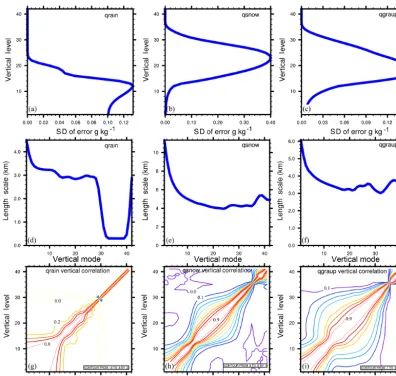
Ne-Figure 3. (a–c)The standard deviations of the background errors at different vertical levels,(d–f)the horizontal correlation length scale as a function of EOF mode, and(g–i)the vertical correlation coefficients forqr,qs, andqg.
braska. The precipitation caused by this convective system lasted for nearly 20 h and ended at approximately 18:00 Z on 2 June 2018.
3.2 Settings of the forecast model
Version 3.9.1 of the Weather Research and Forecasting (WRF; Skamarock et al., 2018) model was employed. All of the experiments were performed on a 450×450×42 domain centered at 41◦N, 96◦W, in eastern Nebraska (Fig. 2). The horizontal grid spacing was 3 km. The terrain-following ver-tical grid was employed with the model top at 50 hPa. All of the experiments used the same physical parameterizations: no cumulus parameterization, the Thompson microphysics scheme (Thompson et al., 2004), the Rapid Radiative Trans-fer Model for general circulation models (RRTMG) long-wave and shortlong-wave radiation scheme (Iacono et al., 2008; Mlawer et al., 1997), and the Unified Noah land-surface model (Chen and Dudhia, 2001). Note that in the current
3.3 Generation of the background error covariance RadarVar was implemented in the WRF data assimilation (WRFDA) (Barker et al., 2012) system. To perform the vari-ational DA with this newly developed radar operator, it is necessary to generate the background error covariance ma-trix withqr,qs, andqgas part of the control variables. The generalized software package for the background error co-variance statistics (GEN_BE) developed by Descombes et al. (2015) was used. The GEN_BE package can generate the univariate background error statistics for 11 variables, including these three hydrometeors. The background error statistics were computed using the National Meteorological Center (NMC) method (Parrish and Derber, 1992), which uses pairs of the differences between the 12 and 24 h fore-casts. In total, 27 d forecasts from 20 May to 15 June 2018 were employed to generate the background error covariance. The background error statistics forqr,qs, andqgare shown in Fig. 3. The vertical distributions of the background error’s standard deviation (Fig. 3a, b, c) are consistent with those of the corresponding hydrometeor profiles: the error of the rainwater mainly appears in the lower levels, while those of snow and graupel mainly exist in the upper levels. The grau-pel may fall from the upper levels into the lower levels, so the graupel error has a broad vertical distribution. The horizontal correlation length scales of the background errors are often less than four grids (<12 km), and the vertical correlation of each hydrometeor can be large at the associated precipitation levels. These spatial correlations of the hydrometeor errors determine the remote horizontal and vertical influences of the observed reflectivity.
3.4 Observation data and verification data
Radar data at 00:00 and 01:00 Z on 2 June 2018 were se-lected to evaluate the radar operator in a variational analysis framework because the convection was sufficiently deep to contain ice-phase species. To fully cover the convective sys-tem at 00:00 Z, data from KABR, KFSD, KLNX, KOAX, KUDX, and KUEX were used, and KLNX was the closest radar from the convective line (Fig. 2). These radars were located in Nebraska and South Dakota. The radar data were stored in level-II format and converted to WRFDA format using a modified 88D2ARPS package, which is widely used in radar DA studies (Putnam et al., 2014; Snook et al., 2011, 2012). During this conversion, the radar data were also hor-izontally remapped to the model grids but remained at the radar elevations in the vertical direction; in other words, the horizontal resolution of the radar data after the conversion was consistent with that of the model. To be consistent with the work using the J08 operator (Jung et al., 2008b), the ob-servation error of the reflectivity was set to 2.0 dBZ. Our early tests using different observation errors indicated that the errors of the analysis reflectivity were comparable when using reflectivity errors ranging from 0.5 to 2.0 dBZ. For
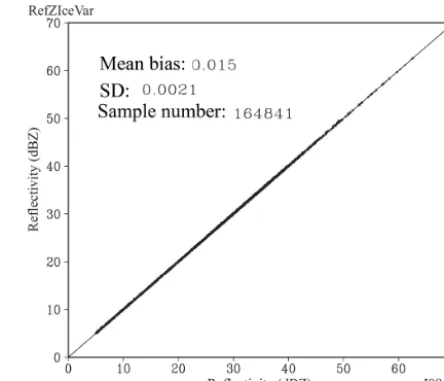
Figure 4.Scatter plot of the reflectivity for J08orig (xaxis) versus RadarVar (yaxis). The bias, standard deviation (SD), and number of samples are listed in the plot.
computational efficiency, we selected the remapped data ev-ery two grids in both thexandydirections for the DA.
The NCEP gridded stage IV (ST4) dataset (Lin and Mitchell, 2005) was used for the precipitation forecast ver-ification. ST4 data with a horizontal resolution of 4 km were interpolated into the 3 km model grid mesh to evaluate the precipitation prediction. At each model grid, the interpolated value was the weighted average of the ST4 data within 10 km of the grid; these data were weighted by the square of the in-verse of the distance between the model grid and the ST4 data location.
3.5 Experimental design
As the first attempt to implement and apply RadarVar in WRFDA, this study focused on the quality of the analysis us-ing the univariate three-dimensional variational (3D-Var) DA method in terms of the root mean square difference (RMSD) against the observed reflectivity and the similarity between the observed reflectivity distributions and the analysis. The forecast performance is the secondary concern and will be explored more thoroughly in a future study with multivariate analysis using more advanced DA techniques.
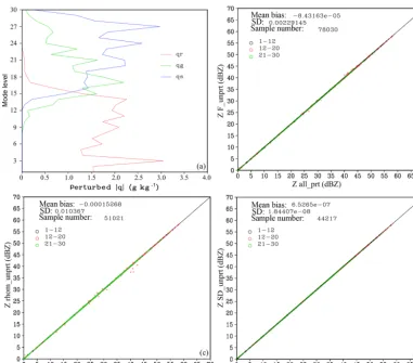
Figure 5. (a)Vertical distributions of the maximum absolute values of the perturbedqr(red),qs(green), andqg(blue). Reflectivity scatter
plots of all_prt (xaxis) versus(b)F_unprt (yaxis),(c)rhom_unprt (yaxis), and(d)SD_unprt (yaxis) at model levels 1–12 (black, lower than 3 km a.g.l.), 12–20 (red, between 3 and 7 km a.g.l.), and 21–30 (green, above 7 km a.g.l.).
100 inner iterations. In each experiment, the radar DA anal-yses were performed at 00:00 and 01:00 Z. The background for the 00:00 Z analysis was interpolated from the GFS anal-ysis with zeros for the hydrometeor fields, and the back-ground for the 01:00 Z analysis was the 1 h WRF forecast from the 00:00 Z analysis with more realistic hydrometeor fields.
Note that TL/AD of RadarVar will not be able to create re-flectivity increments with the zero-hydrometeor background (serves as the base state of TL/AD in the first outer loop), which is the case for the 00:00 Z analysis. An approach to address this issue is to reset the zero background values of
qr, qs, andqg to small values that can range from 10−9 to 10−6kg kg−1 (e.g., Wang and Wang, 2017). However, this approach will result in the fractionF being a constant, while it is expected that F will peak near the middle of the melting layer. Therefore, we introduced a hydrometeor preprocess-ing step before performpreprocess-ing the analysis, which constructs a new background with the weighted sum of the radar-retrieved hydrometeor mixing ratios and their background counter-parts. The hydrometeor retrieval followed the procedure that
is available in WRFDA, which is based on Gao and Sten-srud (2012). The weight coefficients are arbitrarily set to 0.1 for the retrieval part and to 0.9 for the background. The small weight for the retrieval part was used to minimize the impact of the retrieval, mainly to ensure a nonzero background. In addition, current RadarVar cannot work with the weight co-efficient of the retrieval part being smaller than 6×10⁻⁴if the background contains no hydrometeor. A larger weight coef-ficient of the retrieval part (e.g., 0.5) reduces the difference between the background and the observation, which weakens the impact of direct DA using RadarVar and is contradictory to the purpose of this study. The hydrometeor preprocessing was performed at both 00:00 and 01:00 Z in Exp_ref as a ref-erence.
Table 3.Perturbation samples for the verification of the tangent linear operator.
qr(kg kg−1) qs(kg kg−1) qg(kg kg−1) Ratio
Sample 1 min:−4.1×10⁻⁴, max: 4.7×10⁻⁴ min:−4.2×10⁻⁴, max: 4.4×10⁻⁴ min:−3.7×10⁻⁴, max: 3.1×10⁻⁴ 1.00114799 Sample 2 min:−1.6×10⁻⁶, max: 1.8×10⁻⁶ min:−1.6×10⁻⁶, max: 1.7×10⁻⁶ min:−1.4×10⁻⁶, max: 1.2×10⁻⁶ 1.00004709
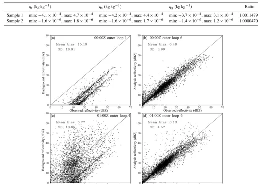
Figure 6.Scatter plots of the observed (xaxis) versus(a, c)background and(b, d)analysis reflectivity at(a, b)00:00 Z and(c, d)01:00 Z in Exp_ref. The mean bias and SD between the observations and the background (or analysis) are listed in each plot.
In several previous studies (Ban et al., 2017; Choi et al., 2017; e.g., Shen and Min, 2015), the horizontal correlation length scale factor of the background error had a large im-pact on the analysis. Therefore, two additional experiments, Exp_ls0.5 and Exp_ls0.125, were performed at 00:00 Z with the length scale factors of 0.5 and 0.125, respectively.
Short-term forecasts from some of these analyses and from the GFS analysis (referred to as the “noDA” experiment) were also carried out and evaluated.
4 Radar operator validation
Before evaluating the performance of RadarVar in WRFDA-3D-Var, we first examined the consistency between J08orig and RadarVar. Because RadarVar follows the J08 operator, the operator implemented in ARPS EnKF (Jung et al., 2008a) was used to serve as the J08orig operator. To be comparable
to J08orig operator, the coefficients of graupel listed in Ta-bles 1 and 2, as well as the intercept parameter and hydrom-eteor density, are replaced by those listed in J08, which were designed for hail. These hail-associated coefficients are used only in Sect. 4 for comparison. The noDA 4 h forecast initial-ized at 00:00 Z was used as the input of the radar operators. The results, which are shown in Fig. 4, indicate that the dif-ference between J08orig and RadarVar is small and accept-able. The small difference is likely caused by the subtle pro-gramming differences between the two software packages.
Figure 7.The(a, e, i, c, g, k)observed (KLNX) and(b, f, j, d, h, l)analysis reflectivities at(a–d)2 km,(e–h)4 km, and(i–l)6 km a.g.l. at
(a, e, i, b, f, j)00:00 Z and(c, g, k, d, h, l)01:00 Z in Exp_ref.
the standard deviation of canting angle, respectively, were unperturbed (i.e., fixed input calculated from the forecast in-put). The test called all_prt denotes that all of the variables in RadarVar were calculated using perturbed mixing ratios. The standard deviation of the perturbation was set to 10 % of the background value; thus, the maximum perturbation could be large, as shown in Fig. 5a. Figure 5 shows that the re-flectivities computed in F_unprt, rhom_unprt, and SD_unprt do not differ significantly from those computed in all_prt. This result indicates that keeping these variables unchanged during the minimization is an acceptable approximation. The most noticeable difference occurs in the middle layer, which is marked in red circles that plot off the diagonal line by sev-eral dBZ (Fig. 5c), but there are few of these samples.
The tangent linear operator of RadarVar was verified through a ratio, which is given by
|H (x+εδx)−H (x)|
ε|H(δx)| =1+O(ε), (30)
where H and H represent the nonlinear operator and the corresponding TL version, respectively, x is the vector of the model state variables (qr,qs,qg), whose perturbation is
denoted byδx, andε is the perturbation magnitude and is greater than zero;δx used the perturbations generated for all_prt. Table 3 shows that the tangent linear operator is suf-ficiently accurate with a ratio close to 1.0.
A correct adjoint operator must satisfy the relationship that is given by
Figure 8.The(a, b, c)00:00 Z and(d, e, f)01:00 Z analyses ofqr(red),qs(green), andqg(blue) at model levels 5 (left column), 15 (middle
column), and 20 (right column) for outer loop 6 in Exp_ref. Model levels 5, 15, and 20 approximately correspond to 0.7, 4.0, and 8.0 km a.g.l., respectively.
5 Results
5.1 Analyses in the observation space and the model space
The Exp_ref analyses (six outer loops, 150 inner iterations, and 0.1 weight for the retrieval part) are first examined in terms of the radar reflectivity and the mixing ratios of rain, snow, and graupel. As expected, the analyzed reflectivity agrees much more closely with the observed reflectivity than the background reflectivity for both analysis times (00:00 and 01:00 Z) (Fig. 6). In addition, considering that the 00:00 Z background bias is much larger than that at 01:00 Z, the comparable analysis error for both times indicates that the analysis is generally relatively insensitive to the initial back-ground. However, a small number of points in the analysis have zero reflectivity, while the corresponding observations can be greater than 10 dBZ (Fig. 6b, d). Further examination indicates that these failed points are related to the locations with very small background values ofqr,qs, andqg, where the nonlinearity of the radar operator and the deficiency of the TL/AD operator are more pronounced.
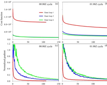
Figure 9.The cost function and normalized gradient norm as functions of the iteration step during the minimization at(a, c)00:00 Z and(b, d)01:00 Z in Exp_ref.
The 00:00 and 01:00 Z analyses ofqr,qs, andqgat three model levels are shown in Fig. 8. The direct assimilation of the reflectivity data using RadarVar successfully retrieved the lower level rain, the upper level snow or graupel, and mixed rain/snow and/or rain/graupel in the melting layer (model level 15). Note that the analysis increment can be created only at levels where the SD of the background error is larger than zero (see Fig. 3).
5.2 Convergence of the minimization
Figure 9 shows the cost function and the norm of its gradi-ent as a function of the number of inner iterations for the first, third, and sixth outer loops. For the 00:00 Z Exp_ref analysis, both the cost function and the gradient norm decrease rapidly in the first outer loop due to the large adjustment from the bad initial background. Using the improved guess after two outer loops, the third outer loop starts from an∼85 % smaller cost function, which is then reduced more gradually with increas-ing iterations. Performincreas-ing more outer loops does not further reduce the cost function substantially, and outer loop 6 even has a slightly larger cost function than that of outer loop 3. Similar behavior can also be observed in the 01:00 Z analy-sis, but performing more than three outer loops can further reduce the cost function to a small extent. This indicates that performing six outer loops may not be necessary and that two or three outer loops may be sufficient.
To more quantitatively measure the impacts of the number of outer loops and inner iterations, the correlation coefficients between the Exp_ref analysis (i.e., six outer loops and 150 it-erations in each loop) and the analyses with one to five outer loops and 50/100/150 inner iterations in each loop are calcu-lated and shown in Fig. 10. In the 00:00 Z analysis, the cor-relation coefficients ofqrandqgare already greater than 0.9 after the first outer loop, and using 50 or 100 inner iterations also results in good agreement with the Exp_ref analysis for
Figure 10.The correlation coefficients ofqr(red),qs(green),qg(blue), and reflectivity (gray) between the Exp_ref analysis (with six outer
loops and 150 inner iterations each loop) and that with different numbers of outer loops and inner iterations at(a)00:00 Z and(b)01:00 Z.
Figure 11.Same as Fig. 6 but for the experiments without hydrometeor preprocessing at(a, b)00:00 and(c, d)01:00 Z.
5.3 Importance of hydrometeor preprocessing
To further investigate the sensitivity of the analysis to the background quality, additional analyses without the hy-drometeor preprocessing step were performed at 00:00 and 01:00 Z. At 00:00 Z, the nonzero background was con-structed by using a very small weight (7×10⁻⁴) for the
Figure 12. (a, c)The analysis reflectivity at 4 km a.g.l. and(b, d)the analyses ofqr(red),qs(green), andqg(blue) at model level 15 at 00:00
and 01:00 Z for the experiments without hydrometeor preprocessing.
These results indicate that the preprocessing step is mostly needed to address the bad background.
Figure 12a shows that the analyzed reflectivity in the melt-ing layer has a reasonable fit to the observations even though it started from very small values of the background reflectiv-ity. The analysis in the model space (Fig. 12b) is also sim-ilar to that with the preprocessing (Fig. 8b). However, the reflectivity coverage (>35 dBZ) in Fig. 12a is smaller than those in the observation and Exp_ref, which corresponds to the horizontally distributed points on the bottom of Fig. 11b. In contrast, the 01Z analysis without the preprocessing step (Fig. 12c, d) closely resembles that with the preprocessing (Figs. 7h and 8e) in terms of the radar reflectivity and hy-drometeor mixing ratios, especially over the strong convec-tive line (dashed black line in Fig. 12d). However, remov-ing this preprocessremov-ing step results in a large spurious echo (marked by “A” in Fig. 12c) that is smaller in Fig. 7h. This implies that the preprocessing step will still be helpful for some “bad” locations (e.g., mismatched convective cells
be-tween the model background and observation) for a generally “good” background.
5.4 Impact of the spatial correlation scale
Figure 13.Same as Fig. 7 but for(a)the observations and the analyses from(b)Exp_ref,(c)Exp_ls0.5, and(d)Exp_ls0.125.
methods, such as 4D-Var and hybrid-3D/4DEnVar that are available in WRFDA.
5.5 Impact on the precipitation forecast
The performance of the precipitation forecasts was quanti-tatively evaluated using the stage IV dataset with the frac-tions skill score (FSS; Roberts and Lean, 2008). Hourly pre-cipitation forecasts between 02:00 and 05:00 Z were evalu-ated because assimilating only the reflectivity is expected to have an impact mostly on the short-term forecast. Similar to Schwartz et al. (2014), the aggregated FSS over the pe-riod from 02:00 to 05:00 Z is shown in Fig. 14 for the fore-casts initialized at 00:00 and 01:00 Z and for different rainfall thresholds. For the forecast from 00:00 Z (Fig. 15a), Exp_ref obtained greater FSSs than those of noDA for thresholds greater than 5 mm h−1with a radius of influence smaller than 40 km. With a larger radius, this difference remains for the lighter rain (<20 mm h−1) but disappears for the heavy rain (≥20 mm h−1). Similar behavior can be observed for the forecast at 01:00 Z (Fig. 15b) but with a more positive
im-pact from the radar DA for heavier rainfall and for a radius of influence smaller than 50 km. Further examination (not shown) indicated that the improvement in the moderate rain (>5 mm h−1) prediction was associated with the larger snow area in the analysis, so the light rain missed by noDA was better captured in Exp_ref. This examination also showed that the higher FSSs obtained by Exp_ref for the heavier rain-fall were mostly associated with the smaller displacement er-ror.
6 Conclusions
in-Figure 14.The FSSs of the hourly precipitation forecasts aggregated over the period from 02:00 to 05:00 Z as functions of the radius of influence for forecasts launched from the(a)00:00 and(b)01:00 Z analyses for Exp_ref (solid lines) and noDA (dashed lines). The hourly precipitation thresholds are denoted by green (1 mm h−1), blue (5 mm h−1), orange (10 mm h−1), and red (20 mm h−1) lines. The straight dashed line represents the skillful FSS at 1 mm h−1.
ner iterations. The results indicated that two to three outer loops with 50–100 iterations in each loop are needed to ob-tain a sufficiently accurate analysis. Two problems of Radar-Var were found in our test. One issue is the analysis failures at locations with observed radar echoes but with zero or ex-cessively small model background values of the hydromete-ors. This issue can be partially resolved using a preprocessing step with radar-retrieved hydrometeors to improve the “bad” background before the analysis. Another issue is the spuri-ous radar echoes (i.e., precipitation) in the analysis caused by the spatial correlations in the background error covariance. These can be reduced by decreasing the correlation length scales. In addition, the short-term (2–5 h) precipitation fore-cast is improved by the direct reflectivity DA even though the inexpensive univariate 3D-Var technique is used in this first attempt of applying RadarVar.
A more thorough evaluation of reflectivity DA with Radar-Var will be examined in a future study using a more ad-vanced hybrid ensemble–variational DA technique, which allows flow-dependent background errors with multivariate correlations and is expected to further reduce the aforemen-tioned deficiencies. Moreover, RadarVar will be extended to include the computation of polarimetric quantities to better determine the phases of the hydrometeors, especially in the melting layers.
Appendix A
This section provides details about the reorganization of all of the terms in the brackets in Eq. (11) in terms of the fwx power. For convenience, the expressions in these brackets are represented byG(fwx).
Applying Eq. (16) to the brackets in Eq. (11) results in
G(fwx)=εx2[A( n X
k=0
Pwxakfwkx) 2+B(
n X
k=0
Pwxbkfwkx) 2
+2C( n X
k=0
Pwxakfwkx)( n X
k=0
Pwxbkfwkx)]. (A1)
Expanding all of the terms of Eq. (A1) results in
G(fwx)=εx2{A n X
i=0
[Pwxai( n X
j=0
Pwxajfi +j wx )]
+B n X
i=0
[Pwxbi( n X
j=0
Pwxbjf i+j wx )]
+2C n X
i=0
[Pwxai( n X
j=0
Pwxbjfi +j
wx )]}. (A2)
Reorganizing the third term (omitting 2C) of Eq. (A2) in terms of thefwxpower (i+j) results in
n X
i=0
[Pwxai( n X
j=0
Pwxbjfi +j
wx )] =Pwxa0Pwxb0fw0x +Pwxa0Pwxb1fw1x+Pwxa1Pwxb0fw1x
· · ·
+Pwxa0Pwxbnfwnx+Pwxa1Pwxb(n−1)fwnx + · · · +PwxanPwxb0fwnx
+Pwxa1Pwxbnfwnx+1+Pwxa2Pwxb(n−1)fwnx+1 + · · · +PwxanPwxb1fwn+1x
· · ·
+Pwxa(n−1)Pwxbnfw2nx−1+PwxanPwxb(n−1)fw2nx−1 +PwxanPwxbnfw2nx
= n X
k=0
[fwkx k X
i=0
PwxaiPwxb(k−i)]
+
2n X
k=n+1
[fwkx n X
i=k−n
PwxaiPwxb(k−i)]. (A3)
The sum functions in the square brackets on the right-hand side of Eq. (A3) correspond to the third expression of Eq. (20). Using the third expression of Eq. (20), the third
term of Eq. (A2) is rewritten as follows:
2C n X
i=0
[Pwxai( n X
j=0
Pwxbjfi +j wx )]
=2C{ n X
k=0
[fwkx k X
i=0
PwxaiPwxb(k−i)]
+
2n X
k=n+1
[fwkx n X
i=k−n
PwxaiPwxb(k−i)]}
=2C
2n X
k=0
PCxkfwkx, (A4)
wherePCxkhas the same meaning as in Eq. (20). Similarly, we can rewrite the other two terms in Eq. (A2) as follows:
A n X
i=0
[Pwxai( n X
j=0
Pwxajfi +j wx )] =
A{ n X
k=0
[fwkx k X
i=0
PwxaiPwxa(k−i)]
+
2n X
k=n+1
[fwkx n X
i=k−n
PwxaiPwxa(k−i)]}
=A
2n X
k=0
PAxkfwkx
B n X
i=0
[Pwxbi( n X
j=0
Pwxbjfi +j wx )] =
B{ n X
k=0
[fwkx k X
i=0
PwxbiPwxb(k−i)]
+
2n X
k=n+1
[fwkx n X
i=k−n
PwxbiPwxb(k−i)]} =
B
2n X
k=0
PBxkfwkx. (A5)
G(fwx)=ε2x(A 2n X
k=0
PAxkfwkx+B 2n X
k=0
PBxkfwkx
+2C
2n X
k=0
PCxkfwkx)
=εx2
2n X
k=0
(APAxkfwkx+BPBxkfwkx+2CPCxkfwkx)
=εx2
2n X
k=0
(APAxk+BPBxk+2CPCxk)fwkx
=εx2
2n X
k=0
Author contributions. SW performed the coding and designed the data assimilation experiments. ZL supervised this study. All authors contributed to the writing of the paper.
Acknowledgements. This work was jointly sponsored by the National Key Research and Development Program of China (2017YFC1502103), the National Natural Science Foundation of China (41505089, 41875129, 41505090, 41430427, and 41805070), the Startup Foundation for Introducing Talent of NUIST (2014R007), and National Key Research and Development Program of China (2018YFC1506404). NCAR is sponsored by the US Na-tional Science Foundation.
Financial support. This work was jointly sponsored by the Na-tional Key Research and Development Program of China (grant no. 2017YFC1502103) and the National Natural Science Foundation of China (grant nos. 41875129, 41430427, and 41805070). NCAR is sponsored by the US National Science Foundation.
Review statement. This paper was edited by Richard Neale and re-viewed by Juanzhen Sun and one anonymous referee.
References
Aydin, K. and Seliga, T. A.: Radar Polarimetric Backscattering Properties of Conical Graupel, J. Atmos. Sci., 41, 1887–1892, 1984.
Ban, J., Liu, Z., Zhang, X., Huang, X.-Y., and Wang, H.: Precipitation data assimilation in WRFDA 4D-Var: im-plementation and application to convection-permitting forecasts over United States, Tellus A, 69, 1368310, https://doi.org/10.1080/16000870.2017.1368310, 2017. Barker, D., Huang, X.-Y., Liu, Z., Auligné, T., Zhang, X., Rugg,
S., Ajjaji, R., Bourgeois, A., Bray, J., Chen, Y., Demirtas, M., Guo, Y.-R., Henderson, T., Huang, W., Lin, H.-C., Michalakes, J., Rizvi, S., and Zhang, X.: The Weather Research and Fore-casting (WRF) Model’s Community Variational/Ensemble Data Assimilation System: WRFDA, B. Am. Meteorol. Soc., 93, 831– 843, 2012.
Borderies, M., Caumont, O., Augros, C., Bresson, É., Delanoë, J., Ducrocq, V., Fourrié, N., Bastard, T. L., and Nuret, M.: Simula-tion of W©-band radar reflectivity for model validaSimula-tion and data assimilation, Q. J. Roy. Meteor. Soc., 144, 391–403, 2018. Caumont, O., Ducrocq, V., Delrieu, G., Gosset, M., Pinty, J.-P.,
Par-ent du Châtelet, J., Andrieu, H., Lemaître, Y., and Scialom, G.: A radar simulator for high-resolution nonhydrostatic models, J. Atmos. Ocean. Tech., 23, 1049–1067, 2006.
Caumont, O., Ducrocq, V., Wattrelot, É., Jaubert, G., and Pradier-Vabre, S.: 1D+3DVar assimilation of radar reflectivity data: A proof of concept, Tellus A, 62, 173–187, 2010.
Chen, F. and Dudhia, J.: Coupling an advanced land surface– hydrology model with the Penn State–NCAR MM5 model-ing system. Part I: Model implementation and sensitivity, Mon. Weather Rev., 129, 569–585, 2001.
Choi, Y., Cha, D. H., and Kim, J.: Tuning of lengthscale and obser-vation error for radar data assimilation using four dimensional variational (4D-Var) method, Atmos. Sci. Lett., 18, 441–448, 2017.
Dawson, D. T., Ii, Xue, M., Milbrandt, J. A., and Yau, M. K.: Comparison of Evaporation and Cold Pool Development be-tween Single-Moment and Multimoment Bulk Microphysics Schemes in Idealized Simulations of Tornadic Thunderstorms, Mon. Weather Rev., 138, 1152–1171, 2010.
Descombes, G., Auligné, T., Vandenberghe, F., Barker, D. M., and Barré, J.: Generalized background error covariance ma-trix model (GEN_BE v2.0), Geosci. Model Dev., 8, 669–696, https://doi.org/10.5194/gmd-8-669-2015, 2015.
Evensen, G.: The ensemble Kalman filter: Theoretical formula-tion and practical implementaformula-tion, Ocean Dynam., 53, 343–367, 2003.
Gao, J. and Stensrud, D. J.: Assimilation of reflectivity data in a convective-scale, cycled 3DVAR framework with hydrometeor classification, J. Atmos. Sci., 69, 1054–1065, 2012.
Hu, M., Xue, M., Gao, J., and Brewster, K.: 3DVAR and cloud anal-ysis with WSR-88D level-II data for the prediction of the Fort Worth, Texas, tornadic thunderstorms. Part II: Impact of radial velocity analysis via 3DVAR, Mon. Weather Rev., 134, 699–721, 2006.
Iacono, M. J., Delamere, J. S., Mlawer, E. J., Shephard, M. W., Clough, S. A., and Collins, W. D.: Radiative forcing by long-lived greenhouse gases: Calculations with the AER radia-tive transfer models, J. Geophys. Res.-Atmos., 113, D13103, https://doi.org/10.1029/2008JD009944, 2008.
Janisková, M. and Lopez, P.: Linearized physics for data assimila-tion at ECMWF, in: Data Assimilaassimila-tion for Atmospheric, Oceanic and Hydrologic Applications, Vol. II, Springer, 2013.
Janisková, M., Thépaut, J.-N., and Geleyn, J.-F.: Simplified and reg-ular physical parameterizations for incremental four-dimensional variational assimilation, Mon. Weather Rev., 127, 26–45, 1999. Johnson, M., Jung, Y., Dawson, D. T., and Xue, M.: Comparison of
simulated polarimetric signatures in idealized supercell storms using two-moment bulk microphysics schemes in WRF, Mon. Weather Rev., 144, 971–996, 2016.
Jung, Y., Zhang, G., and Xue, M.: Assimilation of simulated po-larimetric radar data for a convective storm using the ensem-ble Kalman filter. Part I: Observation operators for reflectivity and polarimetric variables, Mon. Weather Rev., 136, 2228–2245, 2008a.
Jung, Y., Xue, M., Zhang, G., and Straka, J. M.: Assimilation of simulated polarimetric radar data for a convective storm using the ensemble Kalman filter. Part II: Impact of polarimetric data on storm analysis, Mon. Weather Rev., 136, 2246–2260, 2008b. Jung, Y., Xue, M., and Zhang, G.: Simulations of polarimetric radar
signatures of a supercell storm using a two-moment bulk micro-physics scheme, J. Appl. Meteorol. Clim., 49, 146–163, 2010. Kawabata, T., Schwitalla, T., Adachi, A., Bauer, H.-S., Wulfmeyer,
V., Nagumo, N., and Yamauchi, H.: Observational operators for dual polarimetric radars in variational data assimilation sys-tems (PolRad VAR v1.0), Geosci. Model Dev., 11, 2493–2501, https://doi.org/10.5194/gmd-11-2493-2018, 2018.
Liu, C., Xue, M., and Kong, R.: Direct Assimilation of Radar Re-flectivity Data using 3DVAR: Treatment of Hydrometeor Back-ground Errors and OSSE Tests, Mon. Weather Rev., 147, 17–29, 2019.
Mlawer, E. J., Taubman, S. J., Brown, P. D., Iacono, M. J., and Clough, S. A.: Radiative transfer for inhomogeneous atmo-spheres: RRTM, a validated correlated-k model for the longwave, J. Geophys. Res.-Atmos., 102, 16663–16682, 1997.
National centers for environmental information: NEXRAD In-ventory, available at: https://www.ncdc.noaa.gov/data-access/ model-data/model-datasets/global-forcast-system-gfs, last ac-cess: 8 September 2019.
National centers for environmental information: Global Fore-cast System (GFS), available at: https://www.ncdc.noaa.gov/ nexradinv/, last access: 8 September 2019.
Parrish, D. F. and Derber, J. C.: The National Meteorological Center’s spectral statistical-interpolation analysis system, Mon. Weather Rev., 120, 1747–1763, 1992.
Pfeifer, M., Craig, G., Hagen, M., and Keil, C.: A polarimetric radar forward operator for model evaluation, J. Appl. Meteorol. Clim., 47, 3202–3220, 2008.
Posselt, D. J., Li, X., Tushaus, S. A., and Mecikalski, J. R.: Assim-ilation of dual-polarization radar observations in mixed-and ice-phase regions of convective storms: Information content and for-ward model errors, Mon. Weather Rev., 143, 2611–2636, 2015. Putnam, B. J., Xue, M., Jung, Y., Snook, N., and Zhang, G.: The
Analysis and Prediction of Microphysical States and Polarimet-ric Radar Variables in a Mesoscale Convective System Using Double-Moment Microphysics, Multinetwork Radar Data, and the Ensemble Kalman Filter, Mon. Weather Rev., 142, 141–162, 2014.
Ryzhkov, A., Pinsky, M., Pokrovsky, A., and Khain, A.: Polarimet-ric radar observation operator for a cloud model with spectral microphysics, J. Appl. Meteorol. Clim., 50, 873–894, 2011. Schwitalla, T. and Wulfmeyer, V.: Radar data assimilation
experi-ments using the IPM WRF Rapid Update Cycle, Meteorol. Z., 23, 79–102, 2018.
Shen, F. and Min, J.: Assimilating AMSU-A radiance data with the WRF Hybrid En3DVAR system for track predictions of Typhoon Megi (2010), Adv. Atmos. Sci., 32, 1231–1243, 2015.
Skamarock, W. C., Klemp, J. B., Dudhia, J., Gill, D. O., Barker, D. M., Duda, M. G., Huang, X.-Y., Wang, W., and Powers, J. G.: A description of the advanced research WRF version 3, Na-tional Center For Atmospheric Research Boulder CoNCAR/TN-475+STR, 91 pp., 2018.
Snook, N., Xue, M., and Jung, Y.: Analysis of a Tornadic Mesoscale Convective Vortex Based on Ensemble Kalman Filter Assimila-tion of CASA X-Band and WSR-88D Radar Data, Mon. Weather Rev., 139, 3446–3468, 2011.
Snook, N., Xue, M., and Jung, Y.: Ensemble Probabilistic Fore-casts of a Tornadic Mesoscale Convective System from Ensem-ble Kalman Filter Analyses Using WSR-88D and CASA Radar Data, Mon. Weather Rev., 140, 2126–2146, 2012.
Snook, N., Xue, M., and Jung, Y.: Multiscale EnKF Assimilation of Radar and Conventional Observations and Ensemble Forecast-ing for a Tornadic Mesoscale Convective System, Mon. Weather Rev., 143, 1035–1057, 2015.
Sun, J. and Crook, N. A.: Dynamical and microphysical retrieval from Doppler radar observations using a cloud model and its ad-joint. Part I: Model development and simulated data experiments, J. Atmos. Sci., 54, 1642–1661, 1997.
Sun, J. and Wang, H.: Radar data assimilation with WRF 4D-Var. Part II: Comparison with 3D-Var for a squall line over the US Great Plains, Mon. Weather Rev., 141, 2245–2264, 2013. Thompson, G., Rasmussen, R. M., and Manning, K.: Explicit
Fore-casts of Winter Precipitation Using an Improved Bulk Micro-physics Scheme. Part I: Description and Sensitivity Analysis, Mon. Weather Rev., 132, 519–542, 2004.
Tong, M. and Xue, M.: Ensemble Kalman Filter Assimilation of Doppler Radar Data with a Compressible Nonhydrostatic Model: OSS Experiments, Mon. Weather Rev., 133, 1789–1807, 2005. Wang, H., Sun, J., Fan, S., and Huang, X.-Y.: Indirect assimilation
of radar reflectivity with WRF 3D-Var and its impact on predic-tion of four summertime convective events, J. Appl. Meteorol. Clim., 52, 889–902, 2013a.
Wang, H., Sun, J., Zhang, X., Huang, X.-Y., and Auligné, T.: Radar data assimilation with WRF 4D-Var. Part I: System development and preliminary testing, Mon. Weather Rev., 141, 2224–2244, 2013b.
Wang, S: WRFDA_gmdd, available at: https://github.com/ children1985/WRFDA_gmdd, last access: 8 September 2019. Wang, Y. and Wang, X.: Direct assimilation of radar reflectivity
without tangent linear and adjoint of the nonlinear observation operator in the GSI-based EnVar system: Methodology and ex-periment with the 8 May 2003 Oklahoma City tornadic supercell, Mon. Weather Rev., 145, 1447–1471, 2017.
Wattrelot, E., Caumont, O., and Mahfouf, J.-F.: Operational imple-mentation of the 1D+3D-Var assimilation method of radar re-flectivity data in the AROME model, Mon. Weather Rev., 142, 1852–1873, 2014.
Xiao, Q., Kuo, Y.-H., Sun, J., Lee, W.-C., Barker, D. M., and Lim, E.: An approach of radar reflectivity data assimilation and its as-sessment with the inland QPF of Typhoon Rusa (2002) at land-fall, J. Appl. Meteorol. Clim., 46, 14–22, 2007.
Xue, M., Tong, M., and Droegemeier, K. K.: An OSSE framework based on the ensemble square root Kalman filter for evaluating the impact of data from radar networks on thunderstorm analysis and forecasting, J. Atmos. Ocean. Tech., 23, 46–66, 2006. Zhang, G., Vivekanandan, J., and Brandes, E.: A method for
es-timating rain rate and drop size distribution from polarimetric radar measurements, IEEE T. Geosci. Remote S., 39, 830–841, 2001.