https://doi.org/10.5194/gi-6-487-2017
© Author(s) 2017. This work is distributed under the Creative Commons Attribution 3.0 License.
Merging fluxgate and induction coil data to produce low-noise
geomagnetic observatory data meeting the INTERMAGNET
definitive 1 s data standard
Heinz-Peter Brunke1, Rudolf Widmer-Schnidrig2, and Monika Korte1
1GFZ German Research Centre for Geosciences, Telegrafenberg, 14473 Potsdam, Germany 2Black Forest Observatory, Heubach 207, 77709 Wolfach, Germany
Correspondence to:Heinz-Peter Brunke ([email protected]) Received: 3 March 2017 – Discussion started: 15 May 2017
Revised: 8 August 2017 – Accepted: 21 August 2017 – Published: 9 November 2017
Abstract.For frequencies above 30 mHz the instrument in-trinsic noise level of typical fluxgate magnetometers used at geomagnetic observatories usually masks ambient mag-netic field variations on magmag-netically quiet days. This is especially true for stations located at middle and low lat-itudes, where variations are generally smaller than at high latitudes. INTERMAGNET has set a minimum quality stan-dard for definitive 1 s data. Natural field variations referred to as pulsations (Pc-1, Pc-2, Pi-1) fall in this band. Usually their intensity is so small that they rarely surpass the instru-mental noise of fluxgate magnetometers. Moreover, high-quality magnetic field observations in the band 30 mHz– 0.5 Hz contain interesting information, e.g., for the study of ionospheric electron interactions with electromagnetic ion cyclotron plasma waves.
We propose a method to improve 1 Hz observatory data by merging data from the proven and tested fluxgate magne-tometers currently in use with induction coil magnemagne-tometers into a single data stream. We show how measurements of both instruments can be combined without information loss or phase distortion.
The result is a time series of the magnetic field vector com-ponents, combining the benefits of both instruments: long-term stability (fluxgate) and low noise at high frequencies (induction coil). This new data stream fits perfectly into the data management procedures of INTERMAGNET and meets the requirements defined in the definitive 1 s data standard. We describe the applied algorithm and validate the result by comparing power spectra of the fluxgate magnetometer output with the merged signal. Daily spectrograms from the Niemegk observatory show that the resulting data series
re-veal information at frequencies above 30 mHz that cannot be seen in raw fluxgate data.
1 Introduction
Conventional fluxgate magnetometers used at geomagnetic observatories are optimized towards long-term stability as their main purpose. Even though they have excellent proper-ties to measure the low-frequency part of the magnetic spec-trum, their noise usually surpasses the natural background field variations at frequencies higher than 30 mHz at quiet days and mid- or low-latitude observatories. A commonly used instrument is the FGE fluxgate magnetometer (Peder-sen and Merenyi, 2016). However, the demand for low-noise, high-frequency observatory data is increasing. Variations in the band 30 mHz–0.5 Hz correspond to plasma waves, which are important for radiation belt physics. Electrons interacting with such waves can be scattered into the loss cone and re-duce the energy content of the radiation belt. Pc-1 pulsations (f >0.1 Hz) can be caused by electromagnetic ion cyclotron (EMIC) waves, which is the subject of many recent investi-gations (e.g., Shprits et al., 2016 or Usanova et al., 2014).
A quality standard for observatory data has been de-fined in technical note TN6 of 2 October 2014 INTER-MAGNET definitive 1 s data standard (Turbitt, 2014). This INTERMAGNET standard requires a noise level less than 10 pT/
√
noise level at high frequencies have been presented (e.g., Ko-repanov, 2007), it is not desirable to replace approved obser-vatory magnetometers that have proven long-term stability, as long-term absolute stability is the main requirement for geomagnetic observatories. Moreover, it is not desirable to discontinue a long-standing data series.
In the frequency band 30 mHz–0.5 Hz, natural magnetic signals are relatively rare and usually of small intensity. Hence, it is often termed the “dead band” in magnetotel-lurics. Such signals disappear in the noise because of their small intensity. In order to overcome this “blind spot” of magnetometers currently in use, we propose to improve the quality of observatory data by merging fluxgate data with in-duction coil data. At high frequencies inin-duction coils have very little noise but provide no long-term stability. Here we present a method to numerically merge data of both instru-ments. The result is a single time series combining the ben-efits of both instruments: long-term stability (fluxgate) and low noise at high frequencies (induction coil). The result can be understood as 1 s fluxgate data, noise filtered without loss of information on phase or amplitude. The resulting data product fits perfectly in the INTERMAGNET data process-ing scheme established at magnetic observatories. It exceeds the INTERMAGNET noise requirement of 10 pT/
√
Hz at 0.1 Hz by far. As a consequence, three decimal digits of the merged data are valid (1 pT). This is one digit more than re-quired in the INTERMAGNET definitive 1 s data standard. The third digit is needed to describe weak magnetic signals that can now be observed. Otherwise the effect of quantiza-tion noise can be seen in the spectrum as shown in Fig. 3.
2 Noise considerations
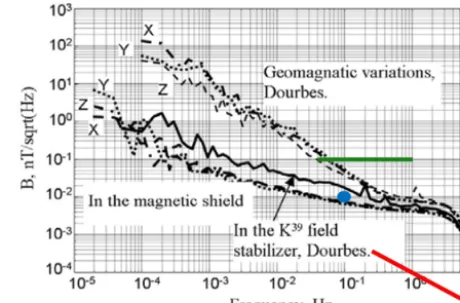
As shown in Figs. 1 and 3, the instrument-inherent noise of a fluxgate magnetometer can be identified in the data as white noise for frequencies above 30 mHz. On a normal day the part of the natural signal with frequencies above 30 mHz van-ishes in the noise. Korepanov (2007) shows a typical power spectral density (PSD) of the natural field at the Dourbes magnetic observatory and compares it to noise of their new magnetometer kept in a shielding box (Fig. 1). We added a green line for the spectral noise density of the FGE in the frequency band 30 mHz–0.5 Hz, as observed at the Niemegk observatory (NGK) and shown in Fig. 3. We marked the IN-TERMAGNET requirement of 10/
√
Hz at 0.1 Hz as a blue dot and added the noise of an induction coil magnetome-ter (MFS05, METRONIX) afmagnetome-ter Ritmagnetome-ter (2001) as a red line. Whereas the fluxgate spectral noise density remains constant at high frequencies, the spectral noise density of an induction coil decreases towards higher frequencies by 20 dB (factor 10) per decade up to a frequency of 100 Hz (Ritter, 2001). At 1 Hz its spectral noise density is at least 2 orders of magni-tudes lower than the noise of any fluxgate magnetometer.
Figure 1.Noise spectra of a magnetometer prototype and of mea-sured natural geomagnetic variations (modified after Korepanov, 2007). We added the high-frequency noise level of the FGE mag-netometer as measured at NGK (green line) and the high-frequency noise of a typical induction coil magnetometer (red line). The blue dot shows the specification required by the INTERMAGNET definitive 1 s data standard (Turbitt, 2014).
Instrument noise at very long periods from days to years is equivalent to instrument long-term stability. This is the most important quality feature of an observatory fluxgate magne-tometer. As described in the following, merging data of both instruments does not in any way effect the long-term stabil-ity.
3 Combining fluxgate and induction coil magnetometer
We take advantage of the fact that the signal of an induction coil magnetometer is proportional to the time derivative of the magnetic field component along the axis of the coil. In the following we consider exemplary theXcomponent. For each sample timet0we look at valuesXFG(ti)registered by the fluxgate magnetometer at timesti varying fromt0−TsN tot0+TsN, with the sample widthTs. Additionally we need recordings of the induction coil at timeti. As result of our algorithm the value BX(t0)is a more precise value of the magnetic field at timet0. The method works comparable to a filter. It acts on the measurements at all timesti varying fromt0−TsNtot0+TsN and produces one output value for timet0. For each newt0the entire process has to be repeated using a new set of 2N+1 measurements. Even though quite a number of measurements are involved, the numerical effort is restricted to just solving the 3×3 matrix of Eq. (5).
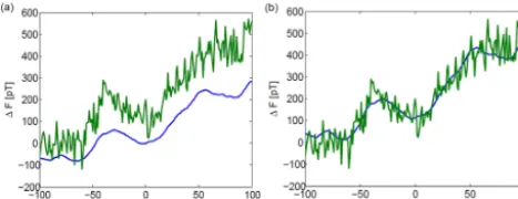
Integrating induction coil data provides a curve which is comparable to the fluxgate data. The integration constant
Fit-Figure 2. (a)Fluxgate data (green) and integral of induction coil signal (blue).(b)Blue curve fitted to FG data by adaptingC,1U andBX(t0)in Eq. (2). In this plot, fluxgate data1F are referred to an arbitrary base value to get handy numerical values on the axis of ordinate.
ting a smooth curve effectively eliminates instrument noise of the fluxgate by averaging. However, the shape of the fitted curve results from the induction coil measurements and the loss of information due to averaging is replaced by informa-tion stemming from the inducinforma-tion coil.
For given timet0and a variable timetiin its environment, data of fluxgate XFG and induction coil magnetometerX˙IC can be expected to satisfy the following equation, assuming that both sensors are aligned with thexaxis:
XFG(ti)−BX(t0)= ti Z
t0 ˙
XIC(t )dt. (1)
Assuming that the induced voltage measured over the induc-tion coil is object to scale factorCand offset1U,
XFG(ti)−BX(t0)= ti Z
t0
(C·UIC(t )+1U )dt. (2)
The blue line in Fig. 2a is achieved by evaluating the inte-gral from the fixed central timet0to a timeti, withivarying from−Nto+Nand applied to an actually measured induc-tion coil data set. The corresponding time series of a fluxgate magnetometer is given as green line.
The blue line (induction coil) is much smoother than the green one (fluxgate data). It can be fitted to the fluxgate data by choosing the right values for the parameters1U,Cand
BX(t0), as shown in the right panel of Fig. 2. For this fit, Eq. (2) has to be solved for1U,CandBX(t0)as unknowns. The effect ofBX(t0)shifts the blue curve vertically,1Utilts it and C changes the amplitudes. With fixed t0 and vary-ingti, Eq. (2) delivers one equation for eachti to determine these unknowns. As shown in Fig. 2 we use a time interval of 200 s. The time spread of 200 s was determined empirically. A longer time interval increases the number of equations and therefore might improve the numerical accuracy of the re-sult. However, the time interval must be small enough to en-sure not to distort the fluxgate signal at lower frequencies. In Sect. 4 we show that a further improvement is not necessary
because the “actual natural” signal is clearly resolved up to the Nyquist frequency of 0.5 Hz.
Assuming that both data series are available at a sample rate of 1 Hz and approximating the integral by a sum, Eq. (2) can be written in the following discrete form:
ti X
t0
(C·UIC(t )+1U )Ts−BX(t0)=XFG(ti). (3)
Assuming thatTs=1 s, one equation is derived for each sam-ple timeti. Ifivaries from−Nto+N, we get the following conditional system for the parameters C, 1U and BX(t0). The system of equations is overdetermined and we have to introduce small residualsri:
C·SN+ 1U·N+ BX(t0)= XFG(tN)+ rN
. . .
C·Si+ 1U·i+ BX(t0)= XFG(ti)+ ri
. . .
C·S−N+ 1U·(−N )+ BX(t0)= XFG(t−N) +r−N.
This is a system of linear equations of the formG·x=y+ r. WithSi=Ts
i−1
P
k=0
UIC(k)and written as explicit matrices,
SN N 1
.. .
Si i 1
.. . S−N −N 1
· C 1U BX(t0)
=
XFG(tN)
.. . XFG(ti)
.. . XFG(t−N)
+ rN .. . ri .. . r−N (4)
C 1U BX(t0)
! = N P
i=−N
Si2
N
P
i=−N
i·Si
N
P
i=−N
Si
N
P
i=−N
i·Si N (N+1)(2N+1)/3 0 N
P
i=−N
Si 0 2N+1
−1 · N P i=−N
SiXFG(ti)
N
P
i=−N
iXFG(ti)
N
P
i=−N
XFG(ti)
. (5)
As a result we get BX(t0), the improved field value at the time t0. Note that the numeric effort for this calculation is very small. It is restricted to the inversion of a 3×3 matrix and calculating six sums in Eq. (5) for each sample of the resulting time series. The sums do not even have to be evalu-ated for each newt0. They can be updated from the previous time step.
4 Results
The success of merging both instruments can best be demon-strated by comparing power spectra of unprocessed FGE and merged data and looking at spectrograms of the respective data series. The induction coil used is a proprietary devel-opment at the NGK. In Fig. 3 PSDs of the fluxgate data as measured in NGK are compared to PSD of merged data. The instrument-inherent noise can clearly be identified in the un-processed data as the white noise (constant noise level) of 0.01 nT2/ Hz for frequencies above 40 mHz. At the same fre-quencies the PSDs of the merged data show a continuing lin-ear decay as expected for the natural field. Very little influ-ence of noise is visible in the PSD of the merged data. At fre-quencies lower than 10 mHz, the spectra of FGE and merged data are identical.
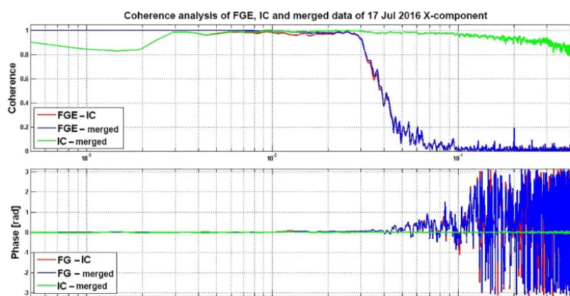
As shown in Fig. 4 the coherence between merged data and FGE data is perfect at low frequencies (<0.01 Hz). At high frequencies (>0.03 Hz) the coherence is very good between merged data and induction coil data. It is not perfect due to the low energy content of the signal at these frequencies. A very high coherence is also observed between FGE and in-duction coil data at frequencies between 0.003 and 0.03 Hz. In this frequency band both instruments are most compara-ble, allowing us to check alignment and intercalibration of both instruments. Induction coils are usually run at a GPS synchronized data logger. This allows us to verify the cor-rect time stamping of the FGE data logger as proposed in the INTERMAGNET definitive 1 s data standard (Turbitt, 2014). For such a test a natural or artificial signal clearly surpassing the FGE white noise level is required.
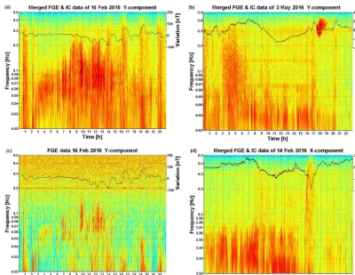
Figure 5 shows spectrograms for 3 selected days. The spectrograms are overlain with time series of the field (black line). Panels (a) and (c) are directly comparable as both cover the 2 February 2016. Panel (a) is based on merged data and panel (c) on fluxgate data only. Whereas in panel (a) the spectral content is clearly resolved up to the Nyquist fre-quency of 0.5 Hz in panel (c) only the strongest activity sur-pass the noise level in the frequency band from 30 mHz up to 0.5 Hz. These are possibly field line resonances and their lowering frequencies towards the nighttime is clearly visible in the merged data in panel (a). Panel (a) also shows with help of the overlain magnetogram that irregular pulsations (Pi-1 pulsation, no clear frequency) are related to the begin-ning of substorms. Panel (b) shows around 18:00 an example of a pulsation event with a clearly defined center frequency of about 300 mHz (Pc-1 pulsation) and panel (d) shows an example of a pulsation whose main frequency rises from about 20 mHz at 15:30 to 400 mHz at 16:30. Additionally, panel (b) shows horizontal structures from 06:00 to 17:00 (16.2 s square wave) and sweeps with falling frequency start-ing at 06:30 and 09:00. Both are manmade contaminations. We found a lot of other remarkable signals revealed in such spectrograms, but discussing them is beyond the scope of this paper.
5 Discussion
Figure 3.Spectra of unprocessed (FGE) and merged data of the entire day (17 July 2016). The level of the fluxgate-inherent white noise is clearly visible for frequencies over 0.04 Hz (blue), whereas the merged data show the continuing decay as expected for the natural field (red).
Figure 4.Coherences between FGE, merged data and induction coil (IC) data. A perfect coherence between merged data and FGE data (blue) is observed at low frequencies (<0.01 Hz). At high frequencies (>0.03 Hz) the coherence is high between merged data and IC data (green).
The INTERMAGNET 1 s standard prescribes a hardware low-pass filter with a corner frequency of 0.2 Hz for the flux-gate data. This filter has absolutely no effect to the result of the merging process. The high-frequency information stems from the induction coil side only. We verified this by numer-ical experiments.
The induction coil data are usually sampled at a rate higher than 1 s−1. These data must be down-sampled numerically to 1 s−1prior to being used in our method. Variometer data are often explored in the time domain. The morphologies of
events like sudden storm commencements, substorms or pul-sations are investigated by visual or automated inspection. In merged data events with even very small amplitudes can be observed, as noise is eliminated to a large extent.
Our method can easily be extended to handle the high sam-ple rate of induction coil data so that the usable signal band-width can be extended up to the 50 Hz power grid frequency – but that is beyond the scope of this paper.
Figure 5.Spectrograms of 3 selected days. Panels(a)and(c)allow for a direct comparison between merged data(a)and fluxgate only(c). Interesting are the irregular pulsations related to substorm activity in panel(a), Pc-1 pulsations with clearly defined frequency of 300 mHz in panel(b)at 18:00 and pulsation activity with rising frequency starting at 15:30 potentially related to EMIC waves in(d).
– We made the assumption that the sensors of the flux-gate and the induction coil magnetometer are perfectly aligned. If this is not the case, the induction coil signal will be affected by the other components. The fitting of both data will worsen. This could be accounted for by numerically rotating the data beforehand. For the deter-mining the rotation matrix a larger data set is needed. The induction coils can be used down to relatively low frequencies, however, so that the overlap with the flux-gate is broad enough to determine the misalignment.
– We assume that the induction coil output is proportional to the time derivative of the magnetic field. Induction coils normally have a ferrite core and use electronic am-plification (Ritter, 2001). Both can influence the linear transfer function in the frequency band from 30 mHz to 1 Hz. This effect could be compensated by a corre-sponding numeric amplitude pre-filtering. This point is especially important if the method should be extended to higher frequencies.
In the process of curve fitting depicted in Fig. 2, it is a good idea to weight points in the direct environment of the time of interest (t0) higher than more remote ones. We have
Figure 6.Data flow of a filtering method to merge fluxgate data and induction coil data. The cutoff frequency of the low-pass fil-ter should be 30 mHz. Calibration of the induction coil data is not included.
had a good experience with a Gaussian filter. For the sake of simplicity we did not include weights in Eqs. (3) to (5).
of induction coil data and the integration constant is elimi-nated by the high-pass filter. In a final step the intermediate result is subtracted from the fluxgate data to get the merged output. The output contains the low-pass-filtered fluxgate data (the high-pass content has been subtracted) and the inte-grated, high-pass-filtered induction coil data. This means that the high-frequency content of the fluxgate, containing mainly noise, is eliminated in the resulting data and replaced by the corresponding high-frequency part of the induction coil side. An advantage of the curve fitting method is that the scale factor of the induction coil is automatically corrected. The numerical effort of the curve fitting method may be slightly higher. Extending the curve fitting method to a higher sam-pling rate of the induction coils (e.g., up to 50 Hz) is straight-forward.
6 Conclusions
We have shown how data of fluxgate magnetometer and in-duction coil data can be merged. A numerical method based on the idea of fitting integrated induction coil data to flux-gate data has been presented in detail. The merged data set combines the excellent long-term stability of well-proven ob-servatory fluxgate magnetometers with the low noise con-tent of induction coil magnetometers at high frequencies. The resulting merged data differ from unprocessed fluxgate data only within the range of the intrinsic fluxgate noise (<0.1 nT). Hence the long-term stability is in no way af-fected. We produce a data set that has the format of usual 1 s fluxgate data but surpasses the specification of the IN-TERMAGNET definitive 1 s data standard by far. The result-ing data set reveals details like Pc-1, Pc-2 and Pi-1 pulsation of even small intensities, which are not resolved by a flux-gate magnetometer. The spectral noise density in the result-ing data set is up to the Nyquist frequency of 0.5 Hz, clearly lower than the spectral density of the natural magnetic field even at days with low activity. Thus with our method we can fill the entire possible bandwidth resulting from the INTER-MAGNET definitive 1 s data standard with meaningful infor-mation about the Earth magnetic field (Turbitt, 2014).
Code and data availability. The MATLAB source code imple-menting the method presented above is available by GFZ Data Ser-vices (Brunke et al., 2017). Test data sets are provided along with the source code. They have kindly been provided by the magnetic observatories Niemegk, Conrad and Eskdalemuir.
Competing interests. The authors declare that they have no conflict of interest.
Special issue statement. This article is part of the special issue “The Earth’s magnetic field: measurements, data, and applications
from ground observations (ANGEO/GI inter-journal SI)”. It is a re-sult of the XVIIth IAGA Workshop on Geomagnetic Observatory Instruments, Data Acquisition and Processing, Dourbes, Belgium, 4–10 September 2016.
Acknowledgements. We thank Sergey Khomutov, Lars Pedersen and one anonymous reviewer. We thank Kusumita Arora for editing. For the provision of test data we acknowledge Roman Leonhard, Ciaran Beggan and Jürgen Matzka. Kirsten Elger helped to publish the software with test data as data object. The article processing charges for this open-access publication were covered by a Research Centre of the Helmholtz Association.
The article processing charges for this open-access publication were covered by a Research
Centre of the Helmholtz Association.
Edited by: Kusumita Arora
Reviewed by: Sergey Khomutov and two anonymous referees
References
Brunke, H.-P., Korte, M., and Widmer-Schidrig, R.: In-dCoilsFGE – A software package for merging Flux-gate and Induction Coil data V.1.0, GFZ Data Services, https://doi.org/10.5880/GFZ.2.3.2017.002, 2017.
Korepanov, V. and Rasson, J.: New INTERMAGNET fluxgate mag-netometer, publications of the institute of geophysics, Pol. Acad. 75 Sc., 398–406, 2007.
Pedersen, L. W. and Merenyi, L.: The FGE Magnetometer and the INTERMAGNET 1 Second Standard, J. Ind. Geophys. Union, 30–36, 2016.
Ritter, O. and Pulz, E.: Entwicklung einer Kalibriereinrich-tung für Induktionsspulenmagnetometer, Scientific Tech-nical Report 01/10 des GeoForschungsZentrum Potsdam, https://doi.org/10.2312/GFZ.b103-0100, 2001.
Schmucker, U. and Weidelt, P.: Electromagnetic In-duction in the Earth, Lectures Notes Aarhus, https://doi.org/10.1038/ncomms12883, 1975.
Shprits, Y., Drozdov, A., and Spasojevic, M.: Wave-induced loss of ultra-relativistic electrons in the Van Allen radiation belts, Nature Communications, 2016.
Turbitt, C.: INTERMAGNET Definitive One-Second Data Standard, INTERMAGNET Technical Note, http://www.intermagnet.org/publications/im_tn_06_v1_0.pdf, 2014.