Efficient Support Vector Machine Classification of Diffuse Large B-Cell Lymphoma and Follicular Lymphoma mRNA Tissue Samples

(1)

Annals. Computer Science Series. 13 Tome 2 Fasc. – 2015

E

F

I

C

I

E

N

T

S

U

P

O

R

T

V

E

C

T

O

R

M

A

C

H

I

N

E

C

L

A

S

I

F

I

C

A

T

I

O

N

O

F

D

I

F

U

S

E

L

A

R

G

E

B

-

C

E

L

Y

M

P

H

O

M

A

N

D

F

O

L

I

C

U

L

A

R

L

Y

M

P

H

O

M

A

M

R

N

A

T

I

S

U

E

S

A

M

P

L

E

S

A

.

W

.

B

a

n

j

o

k

o

11

,

W

.

B

.

Y

a

h

y

a

11

,

M

.

K

.

G

a

r

b

a

11

,

O

.

R

.

O

l

a

n

i

r

a

n

11

,

K

.

A

.

D

a

u

d

a

22

,

K

.

O

.

O

l

o

r

e

d

e

22

1

Department of Statistics, University of Ilorin, P.M.B. 1515, Ilorin, Nigeria

2

Department of Statistics and Mathematical Sciences, Kwara State University, Malete, P.M.B 1530, Ilorin, Nigeria

Corresponding author: W. B. Yahya ([email protected]; [email protected])

ABSTRACT: In this study, an efficient Support Vector Machine (SVM) algorithm that incorporates feature selection procedure for efficient identification and selection of gene biomarkers that are predictive of Diffuse Large B–Cell Lymphoma (DLBCL) and Follicular Lymphoma (FL) cancer tumor samples is presented. The data employed were published real life microarray cancer data that contained 7,129 gene expression profiles measured on 77 biological samples that comprised 58 DLBCL and 19 FL tissue samples. The dimension reduction approach of the Welch statistic was employed at the feature selection phase of the SVM algor ithm. The cost and kernel parameters of the SVM model were tuned over a 10–fold cross-validation to improve the efficiency of the SVM classifier. The entire sample was randomly partitioned into 95% training and 5% test samples. The SVM classifier was trained using Monte Carlo Cross-validation approach with 1000 replications. The performance of this classifier was assessed on the test samples using misclassification error rate (MER) and other performance measures. The results showed that the SVM classifier is quite efficient by yielding very high prediction accuracy of the tumor samples with fewer differentially expressed genes. The selected gene biomarkers in this work can be subjected to further clinical screening for proper determination of their biological relationship with DLBCL and FL tumour sub-groups. However, more studies with large samples might be needed in future to validate the results from this work. KEYWORDS: SVM, Diffuse Large B-Cell Lymphoma, Follicular Lymphoma, 10-fold cross-validation, Welch Statistic.

1. INTRODUCTION

Early identification of cancer tumour in patients has been known to be of great help for efficient management and treatment of such cancer types. However, the management and treatment of cancer tumour largely depends on the specific types of cancer ([Sch05]). Most of the clinical diagnostic methods often require thorough examination of the tumour cell in a microscope before proper diagnoses can take place which obviously might take

considerable longer time before the cancer status of the ailing patients can be determined ([YRU14]). A major consequence of this is the risk of having the cancer tumour (if present in the patient) metastasizes to the neighboring tissue cell areas due to prolonged period of incubation.

One of the most common lymphoid malignancies in adults is Diffuse Large B–Cell Lymphoma (DLBCL) and is curable in less than 50% of patients (Shipp et al. 2002). However, like other forms of cancer tumours, clinical diagnosis of this type of tumor has been reported to be very slow before the true nature of the tumour can be determined. But studies have shown that cancer tumour might be discovered faster with microarray analysis than with clinical methods ([NCG03]; [YOJ12]; [YRU14]). The advent of microarray technology that enables simultaneous investigation of several thousands of gene expression profiles that interact with the tissue samples to produce clinical responses has thrown up additional challenges in the analysis of microarray cancer data. It is a known fact that only few of among the thousands of gene expression signatures are actually biomarkers of the patient’s clinical outcome ([YRU14]). Hence, the need for efficient non-clinical techniques for proper identification and selection of such few biomarker genes becomes necessary.

(2)

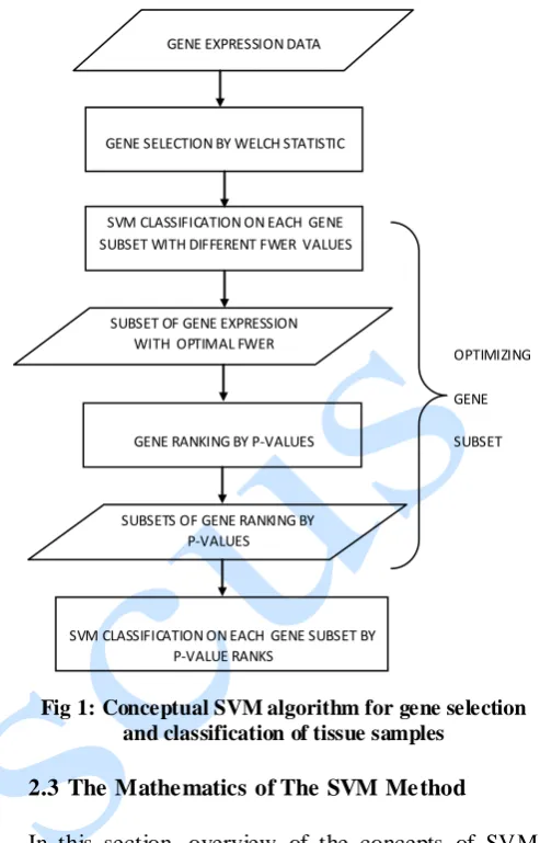
GENE EXPRESSION DATA

GENE SELECTION BY WELCH STATISTIC

SUBSET OF GENE EXPRESSION WITH OPTIMAL FWER SVM CLASSIFICATION ON EACH GENE SUBSET WITH DIFFERENT FWER VALUES

GENE RANKING BY P-VALUES

SUBSETS OF GENE RANKING BY P-VALUES

SVM CLASSIFICATION ON EACH GENE SUBSET BY P-VALUE RANKS

OPTIMIZING

GENE

SUBSET The traditional support vector machine (SVM)

algorithm ([Yah09]; [Ya12]; [Vap95]) has been shown to be very efficient machine learning tool for classification of response groups. SVM has become a state-of-the-art performance in real-world applications such as text categorization, hand written character recognition, image categorization, bio-sequence analysis ([CS12]).

The basic idea behind the SVM method is to construct an optimal separating hyperplane for the two sample groups by mapping the gene expression data to a higher-dimensional space. This involves finding a hyperplane defined by a weight vector wand a bias b such that the separation of the two groups is maximized in a specific sense. Using kernel representations, linear separation in the higher-dimensional space corresponds to a nonlinear decision boundary in the original space.

In this present work, a thorough review of the SVM method for cancer tumour classification in a binary response microarray data problem is presented. Further techniques to improve the classification performance of the original SVM method by incorporating variable selection approaches using different levels of family-wise error rate (FWER) were proposed. The efficiency of this improved SVM algorithm was examined on a published Affymetrix microarray cancer dataset for feature selection and tissue sample classification in a binary response data structure.

2. MATERIAL AND METHODS

2.1 Data Description

The data used in this work are published data set ([S+02]) that contained 7,129 gene expressions profiling on 77 biological subjects. Of these 77 subjects, 58 were diffuse large B-cell lymphoma

(DLBCL) tissue samples while the remaining 19 subjects were follicular lymphoma (FL) tissue samples. The data are freely available and can be

accessed at

www.genome.wi.mit.edu/MPR/lymphoma.

2.2 Flow-Chat o f the Conceptual SVM Feature Selection and Classification Method

The flow-chat of the conceptual SVM feature selected and classification method as employed in this work is presented by Fig 1.

Fig 1: Conceptual SVM algorithm for gene selection and classification of tissue samples

2.3 The Mathematics of The SVM Method

In this section, overview of the concepts of SVM method, its kernel functions, and choice of kernel are presented.

2.3.1 Overview of SVM for hard margin

Given training points such that each input has attributes and is in one of the two classes .Thus, the training dataset is of the

form , where and

. Here, we assume that the data is linearly separable into two classes by drawing a line for D = 2 and a hyperplane for D > 2. Let be the nearest data point to the hyperplane and be the weight vector orthogonal to the hyperplane, then we have the condition that:

(1) For any bias , the equation of the hyperplane can therefore be described by

(3)

To normalize with minimum , it is required that

(3)

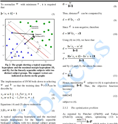
Fig 2: The graph showing a typical separating

hyperplane and the maximal margin hyperplane (H1

and H2) for the linearly separable subjects with two

distinct subject groups. The support vectors are indicated as shown on the graphs

The implementation of SVM boils down to selecting and so that the training data can be describe by

(4)

(5) Equations (4) and (5) above reduced to

(6)

A typical separating hyperplane and the maximal margin hyperplanes for the linearly separable biological subjects with two distinct subject groups are presented by Fig 2.

From Fig 2, the SVM mar gins (distances) that separated the two biological sample groups from the separating hyperplane to the two maximal margin hyperplanes and are denoted by and respectively with . Hence, the main objective of the SVM is to maximize the distance that separated the two sample groups. This is stated by the objective function:

(7) subject to inequality statement in (6).

Let a unit vector of be obtain by

(8) Thus, distance can be computed by

(9) Since is non-negative, therefore

(10) Using (8) in (10), we have that

and by (2) and (3), the above becomes

(11) Hence, maximizing subject to (6) is equivalent to minimizing . Thus, the objective function becomes

(12) subject to (6).

2.3.2 The optimization problem

As reported by Fletcher ([Fle09]) and Yahya ([Yah12]) among others, optimizing (12) is equivalent to which makes it possible to perform the Quadratic Programming (QP) optimization. Hence, the constrained optimization is obtain as

(13)

subject to (6).

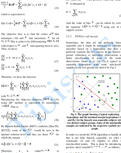
The solution is then obtain by introducing a Lagrange multiplier in the constraint (6) and adding to the objective function as

(4)

(15) which is equivalent to

(16) The objective here is to find the values of that minimizes (16) and that maximizes for all

This is achieve by differentiating

with respect to and and equating them to zero. Thus, we have;

(17)

(18) Therefore, we have the function

(19)

with .

Maximizing the objective function in (19) using QP method is equivalent to minimizing

. That is;

(20) By Karush-Kuhn-Tucker (KKT) condition ([Kar39]; [KT52]), some of the would be zero at the optimal solution level and they are those for which the margin

(21)

Therefore, it is either or

.Since cannot be zero, it shows that equation has to be solved for and .

If then is a support vector (SV). The SVs are the points that defines the plane and margin

for which the ’s are positive. Thus, the value of is obtained by

(22) And the value of bias can be obtain by solving

the equation using any of the

support vectors.

2.3.3 SVM for soft margin

Sometimes, the data are not perfectly linearly separable and it might be necessary to consider a classifier based on a hyperplane that does not perfectly separate the two classes in the interest of greater robustness to individual observations and better classification of most of the tra ining observations James et al. ([J+13]).A typical non-separable hyperplane with some misclassified samples in the two groups are shown by Fig 3.

Fig 3: The graph showing a typical separating

hyperplane and the maximal margin hyperplanes (H1

and H2) for the linearly non-separable subjects with

two distinct subject groups. Some of the misclassified samples are indicated by the respective symbols on the

graph.

In order to extend the SVM algorithm to handle data that is not fully linearly separable, we relax the constraints (4) and (5) slightly to allow for misclassified points. This is done by introducing a positive slack variable as follows;

(23) (24) with . Equations (23) and (24) can be combined to have

(5)

Each of the positive slack variable are called

violations and total violations is ([J+ 13]). The new optimization problem then becomes

(26) Subject to the constraint in(25).

By re-formulating and introducing a new Lagrange multiplier as done in (14) through (19), we have

(27)

Minimizing w.r.t and , and

maximizing it w.r.t each , and we have back the objective function (21) as

subject to the constraint that for . The values of and can then be obtaine d as before.

2.3.4 The kernel function

As a kernel based machine learning algorithm, the four most commonly known SVM kernels are: i.)

The linear kernel: , ii.) The

polynomial kernel: , iii.)

The Radial Basis Function (RBF): and iv.) The

sigmoid: , where

and are the kernel parameters ([Vap95]; [Yah12]).

The concept of kernel, as it relates to the feature space, is considered in order to address the non-linearity problem often encountered in many classification problems. It turns out that the non-linearity in a lower dimensional space is actually linear in a higher dimensional space using a suitable mapping . The SVM algorithm described above only involved the inner products of the

observations (as opposed to the observations themselves) within the kernel setting.

In practice, the optimal SVM and the kernel parameters are obtain through grid search and they are those that give the minimum misclassification error.

In the traditional SVM, the choice of kernel is by trial and error. This involves searching for the best parameters for the four kernels through grid search and applying each of the kernels for classification. The best kernel is the one with minimum misclassification error. But works by Keerthi and Lin ([KL03]) and James et al. ([J+13]) suggest the use of linear kernel when the number of gene chips is larger than the sample size ( ).The RBF kernel performs better for ([H+10]; [KL03]; [Cic15]), while the polynomial kernel contained too many parameters and suffers from numerical difficulties Chih-Jen ([LL03b]). Also, the study by Lin and Lin ([LL03a]) and Chih-Jen ([LL03b]) showed that the sigmoid kernel is not always a valid kernel and does not in any way better than the RBF kernel whenever the RBF works. As a result of the above reasons, our choice of kernels in this study shall be restricted to both the linear and RBF kernels depending on the number of features ( ) and the sample size ( ) in the data.

3. ANALYSIS

The first step to take based on our proposed improved SVM implementation as presented in the flow-chat in Fig 1 is to perform feature selection using the Welch statistic ([Wel47]). This is meant to filter out the numerous noisy and non-informative genes (in univariate sense) in the data. Using the scheme adopted by Mahata and Mahata ([MM07]) for features’ optimization, the remaining few selected informative genes were ranked by their respective p-values as provided by the values of their Welch statistic.

(6)

for (number of gene expressions in the data) where is a modified degrees of freedom of the form

In order to control for the number of false positives in the preliminary gene selection loop of the SVM algorithm, the p-values of the Welch statistic were compared with the Family-Wise-Error rate (FWER)

given by at some

specified nominal Type I error rate in a multiple hypothesis testing for comparing gene variables ([Sid67]). By this, gene would be selected to be differentially expressed if its p-value from the Welch statistic, say is less than (i.e. if ). Various values of (1%, 5%, 10%, 15%, 20% and 100%) were employed in this work for optimal search of differentially expressed genes. The best kernel and SVM parameters were determined through grid search with 10-fold cross-validation for each of the gene subsets selected at each chose values.

The entire sample size was partitioned into 95% training sample which was used to build the SVM classification model and 5% test sample which was used to assess its performance. The SVM algorithm for classification was run over 1000 MCCV runs for each selected gene subsets with the appropriate kernel to ensure model stability.

The subset of genes with the best accuracy was selected as the combination of gene expressions that are most appropriate for the tumor sample classification. As adopted by Mohamad et al. ([M+07]), this subset of genes was ranked based on their respective p-values from the Welch statistic. In order to optimize this feature selection process, the first few genes (i.e. the first 5, first 10, first 15, first 20 and first 25 genes in ranks) from the ranked genes were again re-selected for c lassification of the two tumour groups for optimal results.

The improved SVM algorithm for feature selection and classification was implemented in R statistical package. The R library ‘e1071’ was employed for

the implementation of the SVM method.

4. RESULTS

The results of the improved SVM method for feature selection and classification of the DLBCL and FL tumour groups are presented in this section.

In Table 1, the numbers of gene signatures selected by the selection scheme of the Welch statistic at various chosen FWERs are presented. The SVM algorithm for tissue sample classification was implemented using the linear kernel. This choice of kernel is appropriate for the data since the number of features (7,129 genes) is greater than the sample size (77 samples).

The optimal value of the SVM parameter C at each chosen FWER was determined using 10-fold validation as presented in Table 1. The cross-validation (CV) error rates over all the possible values of the SVM parameter C were computed. The value of C that yielded the least CV error rate becomes the optimal SVM parameter value C at each chosen FWER as indicated in Table 1.

For a clearer overview of the performance of the SVM while tuning the parameter of the SVM, we provide the graph that shows the plot of minimum cross-validation error (misclassification error) rate against the values of the FWER employed for feature selection in Fig 4. The number genes selected at each FWER level are provided in parenthesis on the graph.

Having determined the optimal values of the SVM parameter C at all the chosen levels of the FWER, these were then employed for proper SVM classification using the training data over 1000 Monte-Carlo cross-validation (MCCV) runs. Linear kernel was employed for the SVM implementation since in all the six gene subset cases considered (i.e. at the six chosen FWERs considered). The results of the SVM classification performance over 1000 MCCV runs were presented in Table 2. The table reported the test sample percent correct classification rate (%CCR), misclassification error rate (MER), sensitivity, specificity, positive (+) predictive value, negative (-) predictive value and the Jaccard index of the SVM classifier.

(7)

separately on each of these gene subsets using RBF kernel function (since in all cases). Both the SVM and RBF parameters were tuned for optimality at10-fold cross-validation. The optimal SVM and RBF parameters values as determined from this implementation are provided in Table 3.The optimal parameters values as indicated in Table 3 are the respective parameter values that yielded the minimum CV error rate over 10-fold cross-validation.

The SVM method was implemented using each of the gene subsets and their predetermined respective optimal RBF and SVM parameter values as provided in Table 3 over 1000 MCCV runs. The classification performance of the improved SVM algorithm is presented in Table 4 for various performance indices. The graphs of these performance measures over the five selected gene subsets are presented in Fig 6.

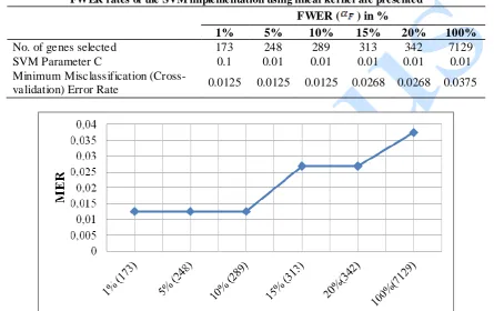
Table 1: Table of selected gene expression profiles by the Welch statistic in the SVM implementation. The optimal SVM parameter values as determined by grid search as well as the minimum cross-validation error rate at each

FWER rates of the SVM implementation using linear kernel are presented

FWER ( ) in %

1% 5% 10% 15% 20% 100%

No. of genes selected 173 248 289 313 342 7129

SVM Parameter C 0.1 0.01 0.01 0.01 0.01 0.01

Minimum Misclassification

(Cross-validation) Error Rate 0.0125 0.0125 0.0125 0.0268 0.0268 0.0375

Fig 4: Graph showing the plot of MER at varying FWERs (in %). The number of genes that yielded the respective MER was indicated in parenthesis along with their respective FWER. The SVM algorithm was run at 10 -fold

cross-validation to tune the parameter of the SVM

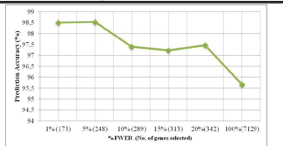
Tables 2: Table of classification results of the SVM method for each gene subset using linear kernel. (*) indicates the FWER level that yielded the best prediction accuracy (highest % CCR of 98.5%)

Assessment Criteria FWER ( ) in %

*1% 5% 10% 15% 20% 100%

No. of genes selected 173 248 289 313 342 7129

CCR (%) 98.50 98.53 97.40 97.23 97.47 95.67 MER 0.0150 0.0147 0.026 0.0277 0.0253 0.0433 Sensitivity 1.0000 1.0000 1.0000 1.0000 1.0000 0.8778 Specificity 0.9808 0.9813 0.9676 0.9654 0.9685 0.9819 Positive Predictive Value 0.9409 0.9412 0.8979 0.8926 0.9001 0.9328 Negative Predictive Value 1.0000 1.0000 1.0000 1.0000 1.0000 0.9609 Jaccard Index 0.9409 0.9412 0.8979 0.8926 0.9001 0.8278

(8)

Fig 5: Graph showing the plot of prediction accuracy (%CCR) at varying FWERs (in %). The number of genes that yielded the respective CCR was indicated in parenthesis along with their respective FWER

Table 3: Results of the optimal values of the tuning parameters of SVM and RBF using the selected genes by p-value ranks. The optimal SVM and RBF parameter values were determined for each of the gene subset by grid search

using the minimum cross-validation error The first set of genes

selected from the ranked genes

RBF kernel parameter

SVM

parameter Minimum CV erro r

γ C

5 3 1 0.0893

10 1 1 0.0911

15 0.0001 10000 0.1018

20 0.01 100 0.0625

25 0.01 100 0.0750

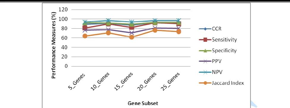
Tables 4: Table of classification results of the SVM method using each selected gene subset by ranks based on RBF kernel

Assessment Criteria No. of genes Employed by p-value ranks

5 10 15 20 25

CCR (%) 89.07 91 87.20 92.50 92.13

MER 0.1093 0.0900 0.1280 0.0750 0.0787 Sensitivity 0.8101 0.8939 0.8207 0.9214 0.9025 Specificity 0.9181 0.9154 0.8888 0.9252 0.9272 Positive Predictive Value 0.7610 0.7766 0.7061 0.8108 0.8033 Negative Predictive Value 0.9402 0.9684 0.9415 0.9701 0.9709 Jaccard Index 0.6419 0.7056 0.6134 0.7594 0.7332

(9)

Fig 6: Graph of the various performance measures over the five selected gene subsets. The number of genes that yielded the respective CCR was indicated in parenthesis along with their respective FWER

5. DISCUSSIONS

This work presents an efficient non-clinical method for classification of Diffuse Large B–Cell Lymphoma and Follicular Lymphoma tumor samples using the expression levels of 7,129 gene signatures.

The fewer numbers of differentially expressed genes selected at each FWER levels indicated that the data contained appreciable number features that are comple x at producing a binary response signal. However, at 1% FWER level, an optimal gene subset with 173 gene signatures was obtained with high prediction accuracy as provided in Table 1. Also, optimal values of the kernel and SVM tuning parameters were determined for each of the gene subsets with linear kernels (for data structures) using 10-fold cross-validation approach as shown in Table 2. The results of the SVM classifier yielded very good prediction performances in terms of (high prediction accuracy, high sensitivity, high specificity, etc.) with fewer differentially expressed genes than when all the genes were employed for classification. This indicates that in the presence of noisy genes, a classifier might not perform as good as when only the most differentially expressed ones among the competing ones are employed by the classification method.

For final gene optimization in order to construct efficient parsimonious SVM classification model, the selected gene subsets at 1% FWER (the optimal value as determined for these data in Table 1) were ranked based on their respective p-values of the Welch statistics. Based on this ranking, the first few gene subsets were selected sequentially to optimize both the SVM and RBF kernel parameters as shown in Table 3.

Similarly, the SVM classification results using each gene subsets as provided in Table 4 indicated the

presence of some false positive genes among those selected at 1% FWER. For example, the prediction accuracy of SVM classifier was about 89% us ing five genes as can be seen in Table 4. This increases to 91% when ten genes were employed by classifiers showing the marginal contribution of the five additional genes. Surprisingly, when fifteen genes were employed, the prediction accuracy of the SVM classifier dropped to around 87%. This is an indication of some false positive (noisy) genes among the new fifteen crop of genes used for classification. Hence, there is the need to further screen the selected gene variables in order to determine those that are actually correlated with the two tumour groups.

Various results of further genes screening as presented in Table 4 revealed the best prediction performance of the improved SVM classifier when twenty differentially expressed genes were employed for classification. In other words, twenty differentially expressed genes are quite sufficient to provide good discrimination between the two tumour groups of DLBCL and FL in the microarray cancer data analyzed in this work.

CONCLUSION

An improved SVM algorithm for tissue sample classification is presented in this work. Efficient scheme to optimize feature selection process for SVM algorithm was equally provided. Various results obtained generally showed that the improved SVM method is quite efficient.

(10)

efficiently determined by grid search over 10-fold cross-validation using the minimum cross-validation errors criteria. This obviously improved the efficiency of the SVM classification results.

Selecting important genes for cancer classification using gene expression data has become inevitable in cancer research, especially when the prime goal is to seek quick diagnosis of the tumour subjects. The conceptual SVM algorithm for gene selection and classification presented in this work has immensely improve the classification and prediction accuracy of the standard SVM method in which all the entire features in the data were used for tumour classification as shown by the SVM results in Table 2. In that result, the best prediction results of the SVM were obtained at 1% FWER using 173 gene variables (CCR = 98.5%; Sensitivity = 100%). However, results of the standard SVM classifier that employed all the 7129 genes provided CCR of 95.67% with Sensitivity of 87.78%.

This work has created opportunity for further research, especially for molecular biologist in the area of investigating into the biological composition of the selected genes regarding their biological relationship to the two tumour groups of Diffuse Large B–Cell Lymphoma and Follicular Lymphoma tumor samples as contained in the data.

REFERENCES

[AY15] Aremu G. T., Yahya W. B. -

Competing Algorithms For Microarray-Based Multiclass Sequential Feature

Selection and Classification.

Proceedings of 4thInternational Science, Technology, Education, Arts, Management & Social Sciences (iSTEAMS) Research Nexus Conference, Nigeria: 675 – 682, 2015. [Cic15] Cichosz P. - Data mining algorithms

explained using R. John Wiley & Sons, N.Y., 2015

[CS12] Cristianini N., Shawe -Taylor J. - An

introduction to support vector

machines. Cambridge University Press, UK, 2012.

[Fle09] Fletcher T. - Support Vector Machines Explained. www.cs.ucl.ac.uk/staff/ T.Fletcher, 2009.

[HCL10] Hsu C.-W., Chang C.-C., Lin C.-J. -

A Practical Guide to Support Vector

Classiﬁcation. Vítor

https://www.scribd.com/vmangaravite Mangaravite, 2010.

[H+12] Hapfelmeier A., Yahya W. B., Rosenberg R., Ulm K. - Predictive modelling of gene Expression data. In:

Handbook of Statistics in Clinical Oncology, 3rd ed., Edited by Crowley, J. and A. Hoering. Chapman and Hall/CRC, New York, 2012, pp., 463-475.

[J+13] James G., Witten D., Hastie T., Tibshirani R. - An Introduction to Statistical Learning with Applications

in R. Springer Science + Business Media New York, 2013.

[Kar39] Karush W. - Minima of functions of several variables with inequalities as side constraints.Master’s thesis, Dept.

of Mathematics, University of Chicago, 1939.

[KL03] Keerthi S. S., Lin C.-J. - Asymptotic

behaviors of support vector

machineswith Gaussian kernel. Neural Computation 15 (7), 1667-1689, 2003. [KT52] Kuhn H. W., Tucker A. W. - Nonlinear

programming. Proc. 2nd Berkeley Symposium on Mathematical Statistics and Probabilities, 481–492, 1952.

[LL03a] Lin H.-T., Lin C.-J. - A Study on Sigmoid Kernels for SVM and the Training of non-PSD Kernels by

SMO-type Methods.

ww.csie.ntu.edu.tw/~cjlin/papers/ tanh.pdf, 2003.

[LL03b] Lin K.-M., Lin C.-J. - A study on reduced support vector machines.IEEE Transactions on Neural Networks. 12: 1449 – 1559, 2003.

[MM07] Mahata P., Mahata K. - Selecting differentially expressed genes using minimu m probability of classification

error. Journal of Biomedical

informatics, 40, 775-789, 2007.

(11)

[NCG03] O’Neill G, Catchpoole D. R., Golemis

E. A. - From correlation to casualty:

microarrays, cancer and cancer

treatment. In: Berrer DP, Dubitzky W, Granzow M, eds. 34:S64-S71, 2003. [Sch05] Schulz W. A. - Molecular Biology of

Human Cancers: An Advanced

Student's Textbook. 1sted. New York: Springer: 1-508, 2005.

[Sid67] Sidak Z. K. - Rectangular Confidence Regions for the Means of Multivariate Normal Distributions. Journal of the American Statistical Association, 62

(318): 626–633.

doi:10.1080/01621459.1967.10482935, 1967.

[S+02] Shipp M. A., Ross K. N, Tamayo P., Weng A. P., Kutok J. L., Aguiar R. C. T., Gaasenbeek M., Angelo M., Reich M., Pinkus G. S., Ray T. S., Koval M. A., Last K. W.., Norton A., Lister T. A., Mesirov J., Neuberg D. S., Lander E. S., Aster J. C., Golub T. R. - Diffuse

large B-cell lymphoma outcome

prediction by gene expression profiling and supervised machine learning. Nature Medicine, 8, 68-74, 2002.

[Tin04] Ting-Lee M.-L. - Analysis of microarray gene expression data. Springer, New York, 2004.

[Vap95] Vapnik V. N. - The Nature of Statistical Learning Theory. New York: Springer-Verlag, 1995.

[Wel47] Welch B. L. - The generalization of "student's" problem when several different population variances are involved. Biometrika 34: 28-35, 1947.

[Yah09] Yahya W. B. - Sequential dimension reduction and prediction methods with high dimensional microarray data. Universitätsbibliothek, Ludwig- Maximilians-Universität, München, Germany. Ph.D. Thesis. URL: http://edoc.ub.uni-muenchen.de/10254/, 2009.

[Yah12] Yahya W. B. - Genes selection and

Tumour Classification in Cancer

Research: A new approach. Säbruck, Germany: Lambert Academic Publishing, 2012.

[YAG15] Yahya W. B., Aremu G. T., Garba M. K. - Multiclass Sequential Feature Selection and Classification Method for Gene Expression Data. Journal of Applied Science and Technology. 20 (1 & 2): 50 – 61, 2015.

[YOJ12] Yahya W. B., Oladiipo M. O., Jolayemi E. T. - A fast algorithm to construct neural networks classification models with high-dimensional genomic data. Annals. Computer Science Series, 10 (1): 39-58, 2012.

[YRU14] Yahya W. B., Rosenberg R., Ulm K. -

Microarray-based Classification of Histopathologic Responses of Locally

Advanced Rectal Carcinomas To

Neoadjuvant Radiochemotherapy

Treatment. Turkiye Klinikleri Journal of Biostatistics, 6(1): 8-23, 2014.